Femtosecond formation of collective modes due to meanfield fluctuations

Abstract

Starting from a quantum kinetic equation including the mean field and a conserving relaxation-time approximation we derive an analytic formula which describes the time dependence of the dielectric function in a plasma created by a short intense laser pulse. This formula reproduces universal features of the formation of collective modes seen in recent experimental data of femtosecond spectroscopy. The presented formula offers a tremendous simplification for the description of the formation of quasiparticle features in interacting systems. Numerical demanding treatments can now be focused on effects beyond these gross features found here to be describable analytically.

The last ten years have been characterized by an enormous activity about ultrafast excitations in semiconductors, clusters, or plasmas by ultrashort laser pulses. The femtosecond spectroscopy has opened the exciting possibility to observe directly the formation of collective modes and quasiparticles in interacting many-body systems. This formation is reflected in the time dependence of the dielectric function Huber et al. (2001, 2002, 2005) or terahertz emission Lloyd-Hughes et al. (2004). For an overview over theoretical and experimental work see Axt and Kuhn (2004); Morawetz (2004). Such ultrafast excitations in semiconductors have been satisfactorily described by calculating nonequilibrium Green’s functions Bányai et al. (1998); Gartner et al. (1999). This approach allows one to describe the formation of collective modes Vu and Haug (2000); Huber et al. (2005) and even exciton population inversions Kira and Koch (2004).

The experimental data in semiconductors like GaAs Huber et al. (2002) or InP Huber et al. (2005) reveal similar features. These features are explained by several numerically demanding calculations. Since some common features are robust, i.e., independent of the actual used material parameters, it should be possible to describe them by a simple theory. The origin of such robust features likely rests in the short- or transient-time behavior itself. At short times higher-order correlations have no time yet to develop, therefore the dynamics is controlled exclusively by mean-field forces.

Based on the mean-field character of the short-time evolution we intend to derive a time-dependent response function from the mean-field linear response. We will start from a conserving relaxation-time approximation which dates back to an idea of Mermin Mermin (1970); Das (1975). Our aim is a simple analytic formula suitable for fits of experimental data.

The electron motion is controlled by the kinetic energy $\hat{\cal E}$, the external perturbation $\hat{V}^{\rm ext}$ and the induced mean-field potential $\hat{V}^{\rm ind}$. The corresponding kinetic equation for the one-particle reduced density matrix $\hat{\rho}$ reads

$$\dot{\hat{\rho}}+i[\hat{\cal E}+\hat{V}^{\rm ind}+\hat{V}^{\rm ext},\hat{\rho}]={\hat{\rho}^{\rm l.e.}-\hat{\rho}\over\tau}$$ (1)

with the relaxation time $\tau$ and a local equilibrium density matrix $\hat{\rho}^{\rm l.e.}$ determined in the following. We will calculate the response in the momentum representation

$$f({p,q},t)=\left\langle p+{q\over 2}\right|\hat{\rho}\left|p-{q\over 2}\right\rangle,$$ (2)

where $\left|p\right\rangle$ is an eigenstate of momentum $p$. For interpretations it is more convenient to transform the reduced density matrix to the Wigner distribution in phase space

$$f({p,R},t)=\sum\limits_{q}{\rm e}^{i{qR}}f({p,q},t),$$ (3)

where $R$ is the spatial coordinate.

The relaxation process in Eq. (1) tends to establish a local equilibrium. Following Mermin, the local equilibrium can be characterized by a local variation of the chemical potential. Up to linear order it can be written as

$$\left\langle p\!+\!{q\over 2}\right|\hat{\rho}^{\rm l.e.}\left|p\!-\!{q\over 2}\right\rangle=f_{p}\delta(q)\!-\!{f_{p\!+\!\frac{q}{2}}\!-\!f_{p\!-\!\frac{q}{2}}\over\varepsilon_{p\!+\!\frac{q}{2}}\!-\!\varepsilon_{p\!-\!\frac{q}{2}}}\delta\mu(q,t)$$ (4)

with the Fermi-Dirac distribution $f_{p}=f_{\rm FD}\left({\varepsilon_{p}}\right)$ and the kinetic energy $\left\langle p+{q\over 2}\right|\hat{\cal E}\left|p-{q\over 2}\right\rangle=\varepsilon_{p}\delta(q)$. The delta function $\delta(q)$ expresses that the corresponding terms are diagonal in momentum or translational invariant. The local deviation $\delta\mu$ from the global chemical potential is selected so that the density of particles is conserved at each point and time instant. Momentum and energy conservations can be included, too, leading to slightly more complicated formulas Morawetz and Fuhrmann (2000a); Atwal and Ashcroft (2002).

Let us now specify $\delta\mu$ from the condition of density conservation which requires that the local equilibrium distribution yields the same density as the actual distribution, $n=\sum_{p}f=\sum_{p}f^{\rm l.e.}$. From Eq. (4) the deviation from the density can be expressed as

$$\delta n(q,t)=\tilde{\Pi}^{\rm RPA}(t,\omega=0)\delta\mu(q,t),$$ (5)

where $\tilde{\Pi}^{\rm RPA}(t,\omega=0)$ is the polarization in random-phase approximation (RPA) at zero frequency with material parameters like electron density and the effective temperature fixed to the value at time $t$. Note that this RPA-polarization enters only the right hand side of (1). The actual polarization which we will derive from (1) is more complex.

The induced potential is given by the Poisson equation

$$V^{\rm ind}({q},t) = \langle p+{q\over 2}|\hat{V}^{\rm ind}|p-{q\over 2}\rangle={e^{2}\over\epsilon_{0}q^{2}}\delta n(q,t).$$ (6)

Now we can solve the kinetic equation (1) for a small external perturbation $V^{\rm ext}$. We split the distribution into the homogeneous part and a small inhomogeneous perturbation, $f(p,q,t)=f_{p}(t)+\delta f(p,q,t)$. Neglecting the time derivative of $f_{p}$ compared to $\delta f$ we can solve Eq. (1) up to linear order in $V^{\rm ext}$

$$\delta f(p,q,t)=i\!\int\limits_{t_{0}}^{t}\!dt^{\prime}\exp{\left[\left(i\varepsilon_{p+\frac{q}{2}}\!-\!i\varepsilon_{p-\frac{q}{2}}\!+\!\frac{1}{\tau}\right)(t^{\prime}-t)\right]}$$

$$\times\Biggl{\{}\left[f_{p+\frac{q}{2}}(t^{\prime})-f_{p-\frac{q}{2}}(t^{\prime})\right]\left[{e^{2}\over\epsilon_{0}q^{2}}\delta n(q,t^{\prime})+V_{q}^{\rm ext}(t^{\prime})\right]$$

$$+{1\over i\tau\tilde{\Pi}^{\rm RPA}(t^{\prime},0)}{f_{p+\frac{q}{2}}(t^{\prime})-f_{p-\frac{q}{2}}(t^{\prime})\over\varepsilon_{p+\frac{q}{2}}-\varepsilon_{p-\frac{q}{2}}}\delta n(q,t^{\prime})\Biggr{\}}$$ (7)

where the perturbation starts at $\delta f(p,q,t_{0})=0$.

The density response, $\chi(t,t^{\prime})$, defined by

$$\delta n(q,t)=\int\limits_{t_{0}}^{t}dt^{\prime}\chi(t,t^{\prime})V_{q}^{\rm ext}(t^{\prime})$$ (8)

follows from Eq. (7) by integrating over $p$ with the result

$$\chi(t,t^{\prime})\!=\!\Pi(t,t^{\prime})\!+\!\!\int\limits_{t^{\prime}}^{t}\!\!d{\bar{t}}\left[\Pi(t,{\bar{t}}){e^{2}\over\epsilon_{0}q^{2}}\!+\!I(t,{\bar{t}})\right]\chi({\bar{t}},t^{\prime}).$$ (9)

Here Mermin’s correction is represented by the term

$$I(t,t^{\prime})={i}\sum\limits_{p}{f_{p\!+\!\frac{q}{2}}(t^{\prime})\!-\!f_{p\!-\!\frac{q}{2}}(t^{\prime})\over\varepsilon_{p\!+\!\frac{q}{2}}-\varepsilon_{p\!-\!\frac{q}{2}}}{{\rm e}^{\left(i\varepsilon_{p\!+\!\frac{q}{2}}-i\varepsilon_{p\!-\!\frac{q}{2}}\!+\!\frac{1}{\tau}\right)(t^{\prime}\!-\!t)}\over\tau\tilde{\Pi}^{\rm RPA}(t^{\prime},0)}.$$

(10)

The polarization,

$$\Pi(t,t^{\prime})\!=\!i\!\sum\limits_{p}[f_{p\!+\!\frac{q}{2}}(t^{\prime})\!-\!f_{p\!-\!\frac{q}{2}}(t^{\prime})]{\rm e}^{\left(i\varepsilon_{\!\!p\!+\!\frac{q}{2}}-i\varepsilon_{\!\!p\!-\!\frac{q}{2}}\!+\!\frac{1}{\tau}\right)(t^{\prime}\!-\!t)},$$ (11)

describes the response of the system with respect to the induced field in contrast to the response function (8) which describes the response of the system with respect to the external field.

To link the derived formulas with familiar results we note that for time-independent $f_{p}$, the Fourier transform of the polarization with respect to the difference time

$$\tilde{\Pi}(T,\omega)=\int d\tau{\rm e}^{i\omega\tau}\Pi(T+\frac{\tau}{2},T-\frac{\tau}{2})$$ (12)

becomes the standard RPA polarization with the frequency argument shifted by the inverse relaxation time

$$\tilde{\Pi}(T,\omega)=\tilde{\Pi}^{\rm RPA}\left(\omega+{i\over\tau}\right).$$ (13)

Moreover, in the limit $t+t^{\prime}\to\infty$ the solution of Eq. (9) approaches the familiar form $\chi=\Pi^{\rm M}/(1-{e^{2}\over\epsilon_{0}q^{2}}\Pi^{\rm M})$ where the Mermin-Das polarization reads Mermin (1970)

$$\Pi^{\rm M}={\tilde{\Pi}^{\rm RPA}(\omega+{i\over\tau})\over 1-i(1+{1\over\omega\tau})\left(1-{\tilde{\Pi}^{\rm RPA}(\omega+{i\over\tau})\over\tilde{\Pi}^{\rm RPA}(0)}\right)}.$$ (14)

Eq. (9) describes how the Mermin susceptibility is formed after a fast release of free carriers.

In the further analysis we will follow closely the experimental way of analyzing the two-time response function Huber et al. (2005). The pump pulse is creating charge carriers in the conduction band at time $t_{0}$ and the probe pulse is sent a time $t_{D}$ later. The time delay after this probe pulse $T=t-t_{D}-t_{0}$ is then Fourier transformed into frequency. Of course everything starts at $t_{0}$ when the pump pulse has created the carriers in the conduction band, i.e. the maximum delay is $T\leq t-t_{0}$. The frequency-dependent inverse dielectric function associated with the actual time $t$ thus reads

$$z(t)={1\over\epsilon(\omega,t)}-1={e^{2}\over\epsilon_{0}q^{2}}\int\limits_{0}^{t-t_{0}}dT{\rm e}^{i\omega T}\chi(t,t-T).$$ (15)

This is exactly the one-sided Fourier transform introduced in Ref. ElSayed et al. (1994). It is worth noting that Wigner’s form of the Fourier transform (12) would just result in a factor of two in the time evolution of the dielectric function.

Now we turn our attention to short times when the response is built up. In general the integral equation (9) together with Eqs. (10) and (11) has to be solved. The useful limit of long wave lengths $q\to 0$ offers an appreciable simplification in that the leading terms of (11) and (10) are $\Pi(t,t^{\prime})\approx{q^{2}n(t^{\prime})\over m}(t^{\prime}-t){\rm e}^{t^{\prime}-t\over\tau}$ and $I(t,t^{\prime})\approx{1\over\tau}{\rm e}^{t^{\prime}-t\over\tau}$. com It is practical to transform the integral equation (9) for the response function directly into one for the inverse dielectric function, Eq. (15), by differentiating twice with respect to time

$$z^{\prime\prime}(t)+({1\over\tau}\!-\!2i\omega)z^{\prime}(t)\!+\!\left[\omega_{p}^{2}(t)\!-\!\omega^{2}\!-\!i{\omega\over\tau}\right]z(t)\!=\!-\omega_{p}^{2}(t)$$

$$z(t_{0})=0;\qquad\left.z^{\prime}(t)\right|_{t=t_{0}}=0.$$ (16)

Here $z^{\prime}(t)=dz(t)/dt$ and we have denoted the time-dependent plasma frequency by $\omega_{p}^{2}(t)={e^{2}n(t)\over\epsilon_{0}\epsilon_{\infty}m}$.

In our simplified treatment the density of electrons $n(t)$ is assumed to be a known function of the time. Due to Rabi oscillations it is a nontrivial function of the laser pulse. If the pulse is short compared to the formation of the collective mode, all details of the density build-up become unimportant and we can approximate the time dependence of the density by a step function ElSayed et al. (1994). Then the plasma frequency is $\omega_{p}(t)=\omega_{p}\Theta(t-t_{0})$, where $t_{0}$ is the time when the pulse reaches its maximum. For this approximation the differential equation (16) can be solved analytically, yielding

$${1\over\epsilon(\omega,t)}=1-{\omega_{p}^{2}\over\Gamma}\int\limits_{0}^{t-t_{0}}dt^{\prime}\,{\rm e}^{(i\omega-{1\over 2\tau})t^{\prime}}\,\sin{(\Gamma t^{\prime})},$$ (17)

where $\Gamma=\sqrt{\omega_{p}^{2}-{1\over 4\tau^{2}}}$. The integral (17) can be expressed in terms of elementary functions, but we find the integral form more transparent.

Formula (17) has been derived from Mermin’s density-conserving approximation. The long-time limit yields the Drude formula

$$\lim\limits_{t\to\infty}{1\over\epsilon}=1-{\omega_{p}^{2}\over\omega_{p}^{2}-\omega(\omega+{i\over\tau})}.$$ (18)

This obvious limit is not so easy to achieve within short-time expansions. For example the approximate result from quantum kinetic theory presented in ElSayed et al. (1994) gives the long-time limit of the form $1-\omega_{p}^{2}/[\omega_{p}^{2}-(\omega+i/\tau)^{2}]$.

In spite of the numerous approximations, Eq. (17) fits well the experimental data, as shown in Fig.  1 for the polar semiconductor GaAs.

The resonance visible at about 8 THz is due to optical phonons. This feature is easily accounted for, see Fig. 1, by adding the intrinsic contribution of the crystal lattice Huber et al. (2002)

$$\epsilon_{\rm GaAs}(\omega,t)=\epsilon_{\infty}\left(\epsilon(\omega,t)+{\omega_{\rm LO}^{2}-\omega_{\rm TO}^{2}\over\omega_{\rm TO}^{2}-\omega^{2}-i\gamma\omega}\right),$$ (19)

with the longitudinal and transversal optical frequencies $\omega_{\rm LO}/2\pi=8.8$ THz and $\omega_{\rm TO}/2\pi=8.1$ THz, the lattice damping $\gamma=$0.2 ps^-1 and the non-resonant background polarizability of the ion lattice $\epsilon_{\infty}=11.0$, see Ref. Huber et al. (2002).

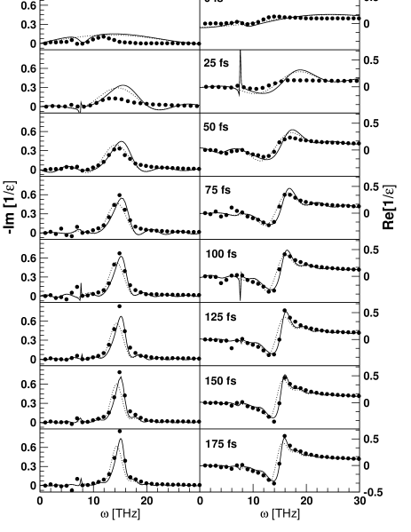
Figure 1: The time evolution of the inverse dielectric function in GaAs. The labels from top to bottom denote the time $t$. The pumb pulse was at $t_{0}=-40$fs and the probe pulse has a full-width at half-maximum of 27$fs$. Circles are data from Huber et al. (2001, 2002), solid lines show the electronic part with intrinsic polarization (19) and dotted lines the electronic part alone (17). The plasma frequency is given by $\omega_{p}=$14.4 THz and the relaxation time is $\tau=85$ fs.

The formula (17) results in a too fast build-up of the collective mode. This is seen in the second row of Fig. 1 at the time $t=25$ fs. This is, however, just the time duration of the experimental pulse and consequently the time of populating the conduction band. Since we have approximated this by the instant jump, this discrepancy at short times around $25$ fs can be expected. A more realistic smooth populating can be modeled by an arctan-function and then the numerical solution of (16) improves the description as we see in Fig. 2. Only the early development is plotted since the later stages agree with the simple estimate (17).

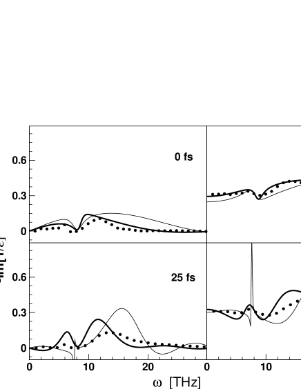
Figure 2: The first two time evolution steps of Fig. 1 comparing the instant population of the conduction band (thin line) with a smooth transition (solid line).

It is obvious that only the gross feature of formation of collective modes can be described by the mean-field fluctuations. For correlations beyond the mean field we should observe deviations. This is the case in the recently observed response of InP Huber et al. (2005), where a coupling between LO phonon and photon modes is reported. In Fig. 3 we see that the formation of the collective mode is delayed in the experiment during the first 100 fs when compared to the mean-field formula (17). Such behavior is due to scattering processes neglected here. At times 100 fs-200 fs the formation of collective modes is described again sufficiently well. For InP we use parameters according to Huber et al. (2005) namely $\omega_{\rm LO}/2\pi=10.3$ THz, $\omega_{\rm TO}/2\pi=9$ THz, $\gamma=0.2$ ps^-1, and $\epsilon_{\infty}=9.6$.

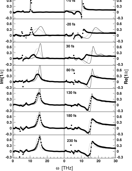
Figure 3: Same as Fig. 1 but for InP. Circles are data from Huber et al. (2005). The plasma frequency and the relaxation time are $\omega_{p}=$14.4 THz and $\tau=77$ fs, respectively and $t_{0}=-70$ fs.

The aim of the present paper was to separate the gross feature of the formation of collective modes at transient times which are due to simple mean-field fluctuations. This has resulted in a simple analytic formula for the time dependence of the dielectric function. Subtracting this gross feature from the data allows one to extract the effects which are due to higher-order correlations and which have to be simulated by quantum kinetic theory Bányai et al. (1998); Gartner et al. (1999); Vu and Haug (2000); Kira and Koch (2004) and response functions with approximations beyond the mean field Kwong and Bonitz (2000). These treatments are numerically demanding such that analytic expressions for the time dependence of some variables Morawetz et al. (1998) are useful for controlling the numerics.

To conclude, we have derived a simple analytic formula for the formation of a collective mode. Being able to describe universal features of the formation of quasiparticles, the simplicity of the presented result is extremely practical and offers a wide range of applications. We see two prominent examples: (1) It could spare a lot of computational power to simulate ultrashort-time behavior of new nano-devices and (2) it can help to understand and describe the formation of collective modes during nuclear collisions which are not experimentally accessible in the early phase of collision.

We thank A. Huber and R. Leitenstorfer for providing us with the experimental data and H. N. Kwong for enlightening and clarifying discussions.

References

- Huber et al. (2001) R. Huber, F. Tauser, A. Brodschelm, M. Bichler, G. Abstreiter, and A. Leitenstorfer, Nature 414, 286 (2001).
- Huber et al. (2002) R. Huber, F. Tauser, A. Brodschelm, and A. Leitenstorfer, phys. stat. sol. (b) 234, 207 (2002).
- Huber et al. (2005) R. Huber, C. Kübler, S. Tübel, A. Leitenstorfer, Q. T. Vu, H. Haug, F. Köhler, and M.-C. Amann, Phys. Rev. Lett. 94, 027401 (2005).
- Lloyd-Hughes et al. (2004) J. Lloyd-Hughes, E. Castro-Camus, M. D. Fraser, C. Jagadish, and M. B. Johnston, Phys. Rev. B 70, 235330 (2004).
- Axt and Kuhn (2004) V. M. Axt and T. Kuhn, Rep. Prog. Phys. 67, 433 (2004).
- Morawetz (2004) K. Morawetz, ed., Nonequilibrium Physics at Short Time Scales - Formation of Correlations (Springer, Berlin, 2004).
- Bányai et al. (1998) L. Bányai, Q. T. Vu, B. Mieck, and H. Haug, Phys. Rev. Lett. 81, 882 (1998).
- Gartner et al. (1999) P. Gartner, L. Banyai, and H. Haug, Phys. Phys. B 60, 14234 (1999); Phys. Phys. B 66, 075205 (2002).
- Vu and Haug (2000) Q. T. Vu and H. Haug, Phys. Phys. B 62, 7179 (2000).
- Kira and Koch (2004) M. Kira and S. W. Koch, Phys. Rev. Lett. 93, 076402 (2004).
- Mermin (1970) N. Mermin, Phys. Rev. B 1, 2362 (1970).
- Das (1975) A. K. Das, J. Phys. F 5, 2035 (1975).
- Morawetz and Fuhrmann (2000a) K. Morawetz and U. Fuhrmann, Phys. Rev. E 61, 2272 (2000a); Phys. Rev. E 62, 4382 (2000b); K. Morawetz, Phys. Rev. B 66, 075125 (2002).
- Atwal and Ashcroft (2002) G. S. Atwal and N. W. Ashcroft, Phys. Rev. B 65, 115109 (2002).
- ElSayed et al. (1994) K. ElSayed, S. Schuster, H. Haug, F. Herzel, and K. Henneberger, Phys. Rev. B 49, 7337 (1994).
- (16) The long wave-length limit corresponds here to the quasiclassical limit, of course. Though we could have started directly with the quasiclassical kinetic equation, we prefer to keep here the more general quantum formalism since the same procedure can be applied for finite systems leading then to explicit quantum corrections.
- Kwong and Bonitz (2000) N. Hang Kwong and M. Bonitz, Phys. Rev. Lett. 84, 1768 (2000).
- Morawetz et al. (1998) K. Morawetz, V. Špička, and P. Lipavský, Phys. Lett. A 246, 311 (1998); K. Morawetz and H. Köhler, Eur. Phys. J. A 4, 291 (1999).