Finite-temperature properties of hard-core bosons confined on
one-dimensional optical lattices

Abstract

We present an exact study of the finite-temperature properties of hard-core bosons (HCB’s) confined on one-dimensional optical lattices. Our solution of the HCB problem is based on the Jordan-Wigner transformation and properties of Slater determinants. We analyze the effects of the temperature on the behavior of the one-particle correlations, the momentum distribution function, and the lowest natural orbitals. In addition, we compare results obtained using the grand-canonical and canonical descriptions for systems like the ones recently achieved experimentally. We show that even for such small systems, as small as 10 HCB’s in 50 lattice sites, there are only minor differences between the energies and momentum distributions obtained within both ensembles.

I Introduction

The study of ultracold quantum gases loaded on optical lattices has become a very active area of experimental and theoretical reseach in recent years. Optical lattices enable enhancing interactions between atoms in weakly interacting Bose-Einstein condensates (BEC’s) and reducing the effective dimensionality of the system. They allow the experimental realization of strongly correlated bosons, well described by the Bose-Hubbard Hamiltonian fisher89 ; jaksch98 , with the consequent observation of the superfluid–Mott-insulator transition greiner02 ; wessel04 . In addition, optical lattices have been used to obtain one-dimensional (1D) systems moritz03 ; tolra04 and to examine the superfluid–Mott-insulator transition in 1D stoferle03 ; batrouni02 .

Due to the strong effects of quantum fluctuations and the possibility of obtaining exact theoretical results, 1D systems are a very attractive laboratory for both experiments and theory. Theoretically, it was shown by Olshanii that in 1D in regimes of large scattering length, low densities, and low temperatures bosons behave as a gas of impenetrable particles known as hard-core bosons (HCB’s) olshanii98 . Such a 1D gas (also recently called a Tonks-Girardeau gas) was introduced by Girardeau, who established an exact mapping between these strongly correlated bosons and noninteracting spinless fermions girardeau60 . Since then 1D HCB’s have been extensively studied by different techniques in both homogeneous lieb63 ; lenard64 ; vaidya79 ; haldane81 ; korepin93 ; cazalilla04_1 and harmonically trapped girardeau01 ; forrester03 ; gangardt04 systems.

The experimental realization of 1D HCB’s followed after more than 40 years of the theoretical introduction of the model paredes04 ; kinoshita04 , with paredes04 and without kinoshita04 an additional lattice along the 1D axis. The additional 1D lattice paredes04 facilitates the achievement of the HCB regime with respect to the continuum case. It allows experimentalists to change the effective mass of the particles and, consequently, the ratio between interaction and kinetic energies paredes04 . Although at very low densities (when interparticle distances are much larger than the lattice spacing) HCB’s on a lattice are equivalent to HCB’s in continuous space, this is not the case for arbitrary fillings cazalilla04 . On 1D lattices the HCB Hamiltonian can be mapped onto the 1D XY model of Lieb, Schulz, and Mattis lieb61 . For periodic systems this model has been also studied extensively in the literature mccoy68 ; vaidya78 ; mccoy83 . More recently, renewed interest has arisen on the properties of HCB’s when additional confining potentials are introduced, as the case relevant to experiments paredes04 .

Remarkably, even in trapped inhomogeneous systems power-law behavior known from the periodic case is present rigol04_1 . The one-particle density matrix exhibits a universal power-law decay with exponent $-1/2$ independent of the power of the confining potential rigol04_1 . These quasi-long-range one-particle correlations generate quasicondensates with occupations scaling proportional to $\sqrt{N_{b}}$ (with $N_{b}$ the number of HCB’s in the system) rigol04_1 . The nonequilibrium dynamics of HCB’s on 1D lattices has also been shown to display very interesting features. Quasicondensates of HCB’s emerge at finite momentum when the system starts its free evolution from a pure Mott-insulating (Fock) state rigol04_2 . In adition, it was shown in Ref. rigol04_3 that in 1D when there is no Mott insulator in the trap, the momentum distribution of expanding HCB’s rapidly approaches that of noninteracting fermions rigol04_3 .

In this work we present an exact study of the finite-temperature properties of HCB’s confined on 1D optical lattices. Following the spirit of Refs. rigol04_1 ; rigol04_2 , we develop an exact numerical approach based on the Jordan-Wigner transformation, which maps HCB’s on a lattice onto noninteracting spinless fermions. We will focus on the effect of temperature on the off-diagonal behavior of one-particle correlations and related quantities like the momentum distribution function $n_{k}$ and the natural orbital occupations. The natural orbitals ($\phi^{\eta}$) are defined as the eigenfunctions of the one-particle density matrix ($\rho_{ij}$) penrose56 ,

$$\sum^{N}_{j=1}\rho_{ij}\phi^{\eta}_{j}=\lambda_{\eta}\phi^{\eta}_{i},$$ (1)

and have occupations $\lambda_{\eta}$. (They resemble one-particle states in these strongly interacting systems.) In dilute higher-dimensional gases, when only the lowest natural orbital (the highest occupied one) scales $\sim N_{b}$, it can be regarded as the BEC order parameter leggett01 . Here we will show that in 1D even at very low temperatures ($T$), when the energy of the system is almost identical to the one at $T=0$, the momentum distribution and the lowest natural orbital occupations can exhibit significant changes with respect to their values in the ground state.

The exposition is organized as follows. In Sec. II we describe our exact approach to study finite-temperature systems. In Sec. III we discuss the properties of HCB’s in a perfect box (an open system). HCB’s confined in harmonic traps are analyzed in Sec. IV. Since in this work we follow a grand-canonical approach to study finite-temperature properties, in Sec. V we compare exact results obtained from a grand-canonical calculation with results obtained from a canonical one for small lattice sizes, like the ones recently achieved experimentally paredes04 . Finally, the conclusions are presented in Sec. VI.

II Exact finite-temperature approach

In this section we detail the exact approach followed to study the finite-temperature properties of HCB’s confined on 1D lattices. The HCB Hamiltonian can be written as

$$H=-t\sum_{i}\left(b^{\dagger}_{i}b_{i+1}+\text{H.c.}\right)+V_{2}\sum_{i}x_{i}^{2}\ n_{i},$$ (2)

with the additional on-site constraints

$$b^{\dagger 2}_{i}=b^{2}_{i}=0,\quad\left\{b_{i},b^{\dagger}_{i}\right\}=1,$$ (3)

which avoid double or higher occupancy. The bosonic creation and annihilation operators at site $i$ are denoted by $b^{\dagger}_{i}$ and $b_{i}$, respectively, and the local density operator by $n_{i}=b^{\dagger}_{i}b_{i}$. The brackets in Eq. (3) apply only to on-site anticommutation relations; for $i\neq j$, these operators commute as usual for bosons $[b_{i},b^{\dagger}_{j}]=0$. In Eq. (2), the hopping parameter is denoted by $t$ and the last term represents a harmonic trap with curvature $V_{2}$.

In order to exactly calculate HCB properties, we use the Jordan-Wigner transformation jordan28

$$b^{{\dagger}}_{i}=f^{{\dagger}}_{i}\prod^{i-1}_{\beta=1}e^{-i\pi f^{{\dagger}}_{\beta}f_{\beta}},\quad b_{i}=\prod^{i-1}_{\beta=1}e^{i\pi f^{{\dagger}}_{\beta}f_{\beta}}f_{i}\ ,$$ (4)

which maps the HCB Hamiltonian onto the one of noninteracting spinless fermions,

$$H_{F}=-t\sum_{i}\left(f^{\dagger}_{i}f_{i+1}+\text{H.c.}\right)+V_{2}\sum_{i}x_{i}^{2}\ n^{f}_{i},$$ (5)

where $f^{\dagger}_{i}$ and $f_{i}$ are the creation and annihilation operators for spinless fermions at site $i$ and $n^{f}_{i}=f^{\dagger}_{i}f_{i}$ is the local particle number operator.

The mapping as presented above is only valid for open systems, as relevant for confined bosons in experiments paredes04 ; kinoshita04 . In such cases HCB’s and fermions have exactly the same spectrum. In order to deal with 1D cyclic chains, with $N$ lattice sites, one needs to consider that

$$b^{\dagger}_{1}b_{N}=-f^{\dagger}_{1}f_{N}\ \exp\left(i\pi\sum^{N}_{\beta=1}n^{f}_{\beta}\right),$$ (6)

so that when the number of particles in the system [$\sum_{i}\langle n_{i}\rangle=\sum_{i}\langle n^{f}_{i}\rangle=N_{b}$] is odd, the equivalent fermionic Hamiltonian satisfies periodic boundary conditions; otherwise, if $N_{b}$ is even, antiperiodic boundary conditions are required in Eq. (5).

Since for finite temperatures we will consider a grand-canonical ensemble—i.e., a system with fluctuating number of particles—in order to avoid the dependence of the equivalent fermionic Hamiltonian on $N_{b}$ we restrict our analysis to the open case. In this case the nontrivial differences between the properties of HCB’s and fermions are only in off-diagonal correlation functions.

For finite temperatures,and within the grand-canonical formalism, the HCB one-particle density matrix can be written in terms of the equivalent fermionic system as

$$\rho_{ij} \equiv \dfrac{1}{Z}\mathrm{Tr}\left\{b^{\dagger}_{i}b_{j}\exp\left[-\left(H-\mu\sum_{l}n_{l}\right)/k_{B}T\right]\right\}$$

$$= \dfrac{1}{Z}\mathrm{Tr}\left\{f^{\dagger}_{i}f_{j}\prod^{j-1}_{\beta=1}\exp(i\pi n^{f}_{\beta})\right.$$

$$\times \left.\exp\left[-\left(H_{F}-\mu\sum_{l}n^{f}_{l}\right)/k_{B}T\right]\prod^{i-1}_{\gamma=1}\exp(-i\pi n^{f}_{\gamma})\right\},$$

where, in addition to Eqs. (4) and (5), we have used the cyclic property of the trace. In Eq. (II), $\mu$ denotes the chemical potential, $k_{B}$ the Boltzmann constant, $T$ the temperature of the system, and $Z$ the partition function

$$Z=\mathrm{Tr}\left\{\exp\left[-\left(H_{F}-\mu\sum_{l}n^{f}_{l}\right)/k_{B}T\right]\right\}.$$ (8)

To calculate traces over the Fock space we will take advantage of the fact that in the equivalent fermionic system Fock states are Slater determinants,

$$|\Psi_{F}\rangle=\prod^{N_{f}}_{i=1}\ \sum^{N}_{j=1}\ P_{ji}f^{{\dagger}}_{j}\ |0\rangle,$$ (9)

with $N_{f}$ the number of fermions and

$${\bf P}=\left(\begin{array}[]{c c c c c c}P_{11}&P_{12}&\cdot&\cdot&\cdot&P_{1N_{f}}\\ P_{21}&P_{22}&\cdot&\cdot&\cdot&P_{2N_{f}}\\ \cdot&\cdot&\cdot&\cdot&\cdot&\cdot\\ \cdot&\cdot&\cdot&\cdot&\cdot&\cdot\\ \cdot&\cdot&\cdot&\cdot&\cdot&\cdot\\ P_{N1}&P_{N2}&\cdot&\cdot&\cdot&P_{NN_{f}}\end{array}\right)$$ (10)

the matrix of the components.

The action of exponentials bilinear on fermionic creation and annihilation operators, as the ones on Eqs. (II) and (8), on Slater determinants generates new Slater determinants muramatsu99 ; assaad02

$$\exp\left(\sum_{ij}f^{\dagger}_{i}X_{ij}f_{j}\right)|\Psi_{F}\rangle=\prod^{N_{f}}_{i=1}\ \sum^{N}_{j=1}\ P^{\prime}_{ji}f^{{\dagger}}_{j}\ |0\rangle,$$ (11)

where

$${\bf P^{\prime}}=e^{\bf X}{\bf P}.$$ (12)

Using this property one can prove the following identity for the trace over the fermionic Fock space muramatsu99 ; assaad02

$$\mathrm{Tr}\left[\exp\left(\sum_{ij}f^{\dagger}_{i}X_{ij}f_{j}\right)\exp\left(\sum_{kl}f^{\dagger}_{k}Y_{kl}f_{l}\right)\cdots\right.$$

$$\left.\qquad\exp\left(\sum_{mn}f^{\dagger}_{m}Z_{mn}f_{n}\right)\right]$$

$$\ \ =\det\left[{\bf I}+e^{\bf X}e^{\bf Y}\cdots e^{\bf Z}\right],$$ (13)

which immediately allows one to calculate the partition function as

$$Z = \det\left[{\bf I}+e^{-({\bf H}_{F}-\mu{\bf I})/k_{B}T}\right]$$ (14)

$$= \prod_{i}\left[1+e^{-(E_{ii}-\mu)/k_{B}T}\right],$$

where ${\bf I}$ is the identity matrix. The last equality was obtained after diagonalizing Hamiltonian (5), ${\bf H}_{F}{\bf U}={\bf UE}$, ${\bf U}$ is the orthogonal matrix of eigenvectors, and ${\bf E}$ is the diagonal matrix of eigenvalues.

The trace in Eq. (II) is calculated along the same line. For $i\neq j$, we notice that

$$f^{\dagger}_{i}f_{j}=\exp\left(\sum_{mn}f^{\dagger}_{m}A_{mn}f_{n}\right)-1,$$ (15)

where the only nonzero element of ${\bf A}$ is $A_{ij}=1$. Then, for $i\neq j$, $\rho_{ij}$ can be obtained as

$$\rho_{ij}=\dfrac{1}{Z} \left\{\det\left[{\bf I}+({\bf I}+{\bf A}){\bf O}_{1}{\bf U}e^{-({\bf E}-\mu{\bf I})/k_{B}T}{\bf U}^{\dagger}{\bf O}_{2}\right]\right.$$ (16)

$$\left.-\det\left[{\bf I}+{\bf O}_{1}{\bf U}e^{-({\bf E}-\mu{\bf I})/k_{B}T}{\bf U}^{\dagger}{\bf O}_{2}\right]\right\}.$$

${\bf O}_{1}$ (${\bf O}_{2}$) is diagonal with the first $j-1$ ($i-1$) elements of the diagonal equal to $-1$ and the others equal to $1$.

The diagonal elements of the one-particle density matrix are the same of noninteracting fermions [see Eq. (II) for $i=j$] and can be easily calculated as muramatsu99 ; assaad02

$$\rho_{ii} = \left[{\bf I}+e^{-({\bf H}_{F}-\mu{\bf I})/k_{B}T}\right]^{-1}_{ii}$$ (17)

$$= \left[{\bf U}\left({\bf I}+e^{-({\bf E}-\mu{\bf I})/k_{B}T}\right)^{-1}{\bf U}^{\dagger}\right]_{ii}.$$

As usual, the chemical potential is fixed using the relation $N_{b}=\sum_{i}\rho_{ii}$ to obtain the desired number of particles in the system.

III Hard-core bosons in a box

In this section we study the finite-temperature properties of HCB’s on a perfect box. In this case the HCB Hamiltonian can be written as

$$H=-t\sum_{i=1}^{N-1}\left(b^{\dagger}_{i}b_{i+1}+\text{H.c.}\right),$$ (18)

with the additional on-site constraints (3).

The above Hamiltonian is particle-hole symmetric, like the one of periodic systems, under the transformation $h_{i}=b^{{\dagger}}_{i},\ h^{{\dagger}}_{i}=b_{i}$ ($h^{{\dagger}}_{i}$ and $h_{i}$ are hole creation and annihilation operators). The particle-hole symmetry implies that the off-diagonal elements of the one-particle density matrix for $N_{b}$ HCB’s [$\rho_{ij}(N_{b})$] and for $(N-N_{b})$ HCB’s [$\rho_{ij}(N-N_{b})$] are identical. Diagonal elements satisfy the relation $\rho_{ii}(N_{b})=1-\rho_{ii}(N-N_{b})$. This leads to a momentum distribution function

$$n_{k}=\dfrac{1}{N}\sum_{jl}e^{-ik(x_{j}-x_{l})}\rho_{jl},$$ (19)

which satisfies the relation

$$n_{k}(N_{b})=n_{-k}(N-N_{b})+\left(1-\frac{N-N_{b}}{N/2}\right).$$ (20)

In contrast to periodic systems where the natural orbitals [Eq. (1)] are momentum states forrester03 ; rigol04_1 , this is not the case in a box. (The system is not translationally invariant.) In Fig. 1 we show the lowest-natural-orbital wave function in a box at different temperatures. We have normalized it as

$$\varphi^{0}=R^{1/2}\phi^{0},\quad R=\left(N_{b}N\right)^{1/2},$$ (21)

so that $\varphi^{0}$ vs $x/N$ is independent of the system size when the density $\rho=N_{b}/N$ is kept constant.

Figure 1: Wave function of the lowest natural orbital at different temperatures in half-filled systems with 1000 lattice sites.

Figure 1 shows that at finite temperatures the weight of the lowest natural orbital increases in the center of the system, departing from the constant value it would have in the periodic case ($k=0$ state). Still, we find that qualitatively (and quantitatively) the natural orbital occupations behave very similarly to the occupations of the momentum states so that for the box we will restrict our analysis to $n_{k}$. The natural orbitals will be relevant to the discussion in the harmonic trap where their behavior can be qualitatively different to the one of $n_{k}$.

In Figs. 2(a)–2(c) we show the HCB momentum distribution function for half-filled systems with $N=1000$ and different temperatures. We have plotted as dashed lines the ground-state results for comparison. The effects of small but finite temperatures are dramatic. This can be better seen in Figs. 2(a) and 2(b) where the energies of the finite-temperature systems are almost identical to the ones of the ground state. For $k_{B}T=0.01t$, the relative energy difference $(\delta E=[E(T)-E(0)]/|E(0)|)$ between the finite-temperature system [$E(T)$] and the ground state [$E(0)$] is $\delta E\sim 0.01\%$. In Fig. 2(a) one can see that the $k=0$ momentum peak is already around 2/3 of the one at zero temperature. For the case in Fig. 2(b), $\delta E\sim 0.4\%$ and the peak at $n_{k=0}$ has already reduced almost 5 times. At $k_{B}T=0.5t$ in Fig.(a), the zero momentum peak has practically disappeared.

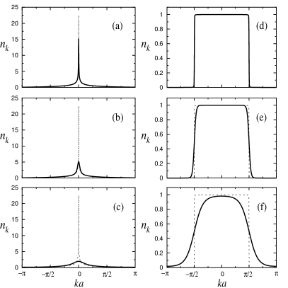
Figure 2: Momentum distribution function of HCB’s (a)–(c) and noninteracting fermions (d)–(f) for half-filled systems with 1000 lattice sites at different temperatures (solid line). The temperature [energy] of the system in each case is $k_{B}T=0.01t$ [$E=-6.362\times 10^{2}t$] (a),(d), $0.10t$ [$-6.336\times 10^{2}t$] (b),(e), and $0.50t$ [$-5.585\times 10^{2}t$] (c),(f). The dashed line in all the figures depicts the ground-state result ($E=-6.363\times 10^{2}t$).

As opposed to the HCB momentum distribution function, we have plotted in Figs. 2(d)–2(f) the momentum distribution function of the equivalent noninteracting fermions. These figures not only show the differences between the shape of the momentum distributions in both cases, but also the fact that they are affected very differently by the temperature. In the fermionic case it is well known that the changes on $n_{k}$ occur only around the Fermi surface and are of order $k_{B}T$, so that in Fig. 2(d) one cannot notice the differences between the finite- and zero-temperature cases. In Fig. 2(e) they are very small, and only when $k_{B}T$ becomes of the order of $t$ [Fig. 2(f)] can one see a large deviation of the finite-temperature $n_{k}$ with respect to the one in the ground state.

The zero-temperature peaks in the HCB $n_{k}$ [Figs. 2(a)–Figs. 2(c)] reflect the presence of quasi-long-range one-particle correlations mccoy68 ; vaidya78 ; mccoy83 ; rigol04_1 ; i.e., there is a power-law decay $\rho_{ij}\sim|x_{i}-x_{j}|^{-1/2}$. In these 1D systems any finite temperature generates an exponential decay of $\rho_{ij}$, which destroys the quasi-long-range correlations present in the ground state. This exponential decay is the one producing dramatic effects in $n_{k}$.

In Fig. 3 we show the decay of one-particle correlations for the same systems of Fig. 2. At very low temperatures ($k_{B}T=0.01t$) the one-particle density matrix follows the ground-state result over a certain distance, which reduces with increasing the temperature, approximately up to the point where the exponential decay sets in. Our results in Fig. 3 can be compared with the ones obtained by other means for $\left\langle S^{x}_{i}S^{x}_{j}\right\rangle$ in the 1D spin-1/2 isotropic XY model tonegawa81 , to which HCB’s can be mapped. Apart from a (1/2) normalization factor the results agree.

Figure 3: Decay of the one-particle density matrix at different temperatures in half-filled systems with 1000 lattice sites. Thin solid lines following finite-temperature results exhibit exponential decays, while the one following the $T=0$ result exhibits a power-law decay $\sim x_{i}^{-1/2}$. In all cases we measured $\rho_{ij}$ fixing $j$ in the middle of the box—i.e., $x_{j}=0$

The quantity of relevance to characterize the finite-temperature exponential decay of the one-particle density matrix $\rho_{ij}\sim e^{-|x_{i}-x_{j}|/\xi}$ (Fig. 3) is the correlation length $\xi$. This quantity is of experimental importance since for $\xi\gtrsim N$ the HCB gas (essentially) exhibits at finite temperatures properties of the ground state. At low temperatures, $k_{B}T<t$, the correlation length decreases as $\xi\sim 1/T$ with increasing temperature. This is shown in Fig. 4.

Figure 4: Correlation length vs temperature (in units of $t$) in half-filled systems with 1000 lattice sites. We have plotted $\xi$ as a thick solid line and the second moment of the one-particle density matrix $\tilde{\xi}$ as a dashed line (see text). The thin solid line is the result of a fit $\xi/a=1.27t/k_{B}T$.

A way of seeing the effects that a finite-temperature correlation length produces in these bosonic systems is to study how the occupation of the zero-momentum state scales with the number of particles (or the system size) when the density is kept constant. Results for $n_{k=0}$ vs $N_{b}$ are presented in Fig. 5. There we have plotted results for as many temperatures as in Fig. 3 so that one can see at what system size the finite-temperature results depart from the ones of the ground state. Since the system size is twice the number of particles (they are at half filling), one can then notice, with the help of Fig. 4, that the mentioned departure indeed occurs for system sizes larger than the correlation length. For example, a half-filled box with 20 HCB’s (a filling similar to the one achieved experimentally in Ref. paredes04 ) would have a momentum distribution function very similar to the one in the ground state up to a temperature $k_{B}T=0.05t$. At zero temperatures $n_{k=0}$ scales proportionally to $\sqrt{N_{b}}$; i.e, it diverges when $N_{b}\rightarrow\infty$, reflecting the power-law decay of one-particle correlations shown in Fig. 3 rigol04_1 .

Figure 5: Scaling of $n_{k=0}$ vs $N_{b}$ for a constant density $\rho=0.5$ and the same values of the temperature chosen in Fig. 3.

The one-particle correlation length not only depends strongly on the temperature, but also on the density in the system. (In Fig. 4 we have only shown results for the half-filled case.) The dependence of the correlation length on the density, for two values of the temperature, is depicted in Fig. 6. Notice that both curves are symmetric with respect to $\rho=0.5$ due to particle-hole symmetry.

Figure 6: Correlation length vs density for systems with $N=500$, $k_{B}T=0.1t$ (solid line) and $k_{B}T=0.5t$ (dash-dotted line). Thick lines depict $\xi$ and thin lines the second moment of the one-particle density matrix $\tilde{\xi}$.

The strong dependence of the correlation length on the density represents a difficulty for defining $\xi$ in inhomogeneous systems, like the ones achieved experimentally where HCB’s are trapped in harmonic confining potentials. (In a box the density is not exactly constant, away from half and integer fillings, due to Friedel oscillations, but they reduce with increasing system size.) An alternative definition to the correlation length $\xi$ may be given as the second moment of the one-particle density matrix

$$\tilde{\xi}=\sqrt{\dfrac{1}{2}\dfrac{\sum_{ij}\left(x_{i}-x_{j}\right)^{2}\rho_{ij}}{\sum_{ij}\rho_{ij}}}.$$ (22)

In Fig. 4 we have plotted $\tilde{\xi}$ along with $\xi$. When $1<\xi\ll N$ both $\tilde{\xi}$ and $\xi$ are very similar. For the lowest temperatures, in Fig. 4, we considered systems with 1000 lattice sites, which are not much larger than the correlation length. This is the origin of the differences between $\tilde{\xi}$ and $\xi$ observed for large values of $\xi$. At high temperatures ($k_{B}T>t$) the value of $\tilde{\xi}$ is completely dominated by the very-short-distance sector of the one-particle density matrix, so that $\tilde{\xi}$ and $\xi$ are expected to be very different. At intermediate temperatures one can use $\tilde{\xi}$ as a good estimate of $\xi$.

In Fig. 6 we have also plotted $\tilde{\xi}$ along with $\xi$ so that one can realize how the inclusion of the short-range part of the one-particle density matrix in $\tilde{\xi}$ produces different effects for low densities, where $\tilde{\xi}>\xi$, and high densities, where $\tilde{\xi}<\xi$. Still the overall behavior of $\tilde{\xi}$ is similar to the one of $\xi$. In the next section we will rely on $\tilde{\xi}$ for estimating the correlation length in harmonic traps and also for comparing it to the one in the box.

IV Hard-core bosons in harmonic traps

We study in this section HCB’s trapped in harmonic potentials. The addition of a confining potential generates a position-dependent density profile where, at zero temperature, superfluid and Mott-insulating regions can coexist. In the next two subsections we analyze the effects of the temperature on density and momentum profiles of systems in which the ground state is (i) superfluid (Sec. IV.1) and (ii) a coexistence of superfluid and Mott-insulating phases (Sec. IV.2). In Sec. IV.3 we address more general questions like the behavior of one-particle correlations and scaling properties at finite temperatures.

In harmonic traps we normalize $n_{k}$ using a length scale set by the combination lattice-confining potential,

$$\zeta=\left(V_{2}/t\right)^{-1/2},$$ (23)

so that

$$n_{k}=\dfrac{a}{\zeta}\sum^{N}_{jl=1}e^{-ik(j-l)}\rho_{jl}.$$ (24)

In addition, instead of the density $\rho=N_{b}/N$, relevant to the periodic or open case, we consider the characteristic density rigol04_1 ; rigol03_3

$$\tilde{\rho}=N_{b}a/\zeta.$$ (25)

As shown in Ref. rigol03_3 up to $\tilde{\rho}\sim 2.6$–2.7 there is no Mott insulator in the trap. For larger values of $\tilde{\rho}$ a Mott-insulating phase appears in the middle of the system.

IV.1 Superfluid case at $T=0$

In Fig. 7 we show density and momentum profiles in a trap with 200 HCB’s ($\tilde{\rho}=2$) for different temperatures (solid line) and compared to the ground-state case (dashed line). As for the fermionic $n_{k}$ in Figs. 2(d)–2(f), the changes of the density profiles with the temperature in Figs. 7(a)–7(c) are the ones expected for fermions. [HCB’s and fermions exhibit identical density profiles, Eq. (II).] For temperatures much smaller than the Fermi energy, which is of the order of $t$ for these systems, the density profiles almost do not change. The same occurs with the total energy $E$ of the trapped cloud, as seen from their values reported in the caption of Fig. 7. On the other hand, the behavior of $n_{k}$, related to off-diagonal one-particle correlations, is very different to the one of the density. At $k_{B}T=0.01t$ [Figs. 7(a) and 7(d)], when the energy of the system has changed by $0.03\%$ with respect to the ground-state energy, changes can be already noticed in $n_{k}$ around $k=0$. For $k_{B}T=0.1t$ [Figs. 7(b) and 7(e)], the energy is $3\%$ larger than in the ground state and the peak in $n_{k=0}$ is less than one-third of its value at $T=0$. For larger temperatures, like $k_{B}T=0.5t$ in Figs. 7(c) and 7(f), almost no peak can be seen in $n_{k=0}$ as compared with the one in the ground state. This is similar to the results obtained for the box in the previous section, with a difference being that in the box the density distribution is not affected by the temperature.

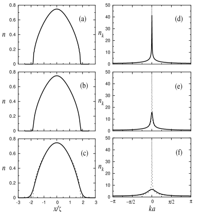
Figure 7: Density (a)–(c) and normalized momentum distribution function (d)–(f) of 200 HCB’s in a trap with $V_{2}a^{2}=10^{-4}t$ ($\tilde{\rho}=2$) at different temperatures (solid line). The temperature [energy] of the system in each case is $k_{B}T=0.01t$ [$E=-37.71t$] (a),(d), $0.10t$ [$-36.44t$] (b),(e), and $0.50t$ [$-8.48t$] (c),(f). The dashed line in all the figures depicts the ground-state result ($E=-37.72t$).

Other quantities of relevance to the harmonically trapped case are the natural orbital occupations [Figs. 8(a)–8(c)] and the wave function of the lowest natural orbital [Figs. 8(d)–8(f)]. In Figs. 8(d)–8(f) we normalize the natural orbital wave function following Ref. rigol04_3

$$\varphi^{0}=R^{1/2}\phi^{0},\quad R=\left(N_{b}\zeta/a\right)^{1/2}.$$ (26)

Like $n_{k}$, the natural orbital occupations exhibit a very strong dependence on the temperature, which can be understood since they are also related to the off-diagonal one-particle correlations. More interesting, and qualitatively different to the case in the box, is the behavior displayed by the lowest-natural-orbital wave function in Fig. 8. With increasing temperature, for large fillings, the weight of the lowest natural orbital in the middle of the trap decreases, and for $k_{B}T=0.5t$ [Fig. 8(f)] it is exactly zero. This behavior of the wave function is accompanied by the appearance of a degeneracy in the occupation of the lowest natural orbitals. These two effects are very similar to the ones generated by the increase of the filling in the ground state of the system and the formation of a Mott insulator in the middle of the trap rigol04_1 . However, as seen in Figs. 7(a)–7(c) no Mott insulator is created by an increase of the temperature.

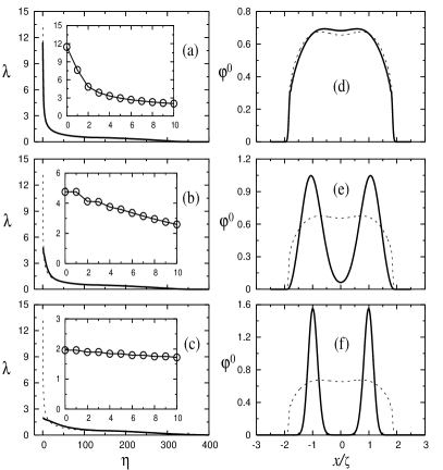
Figure 8: Natural orbital occupations (a)–(c) and normalized wave function of the lowest natural orbital (d)–(f) for the same systems shown in Fig. 7, $N_{b}=200$ and $V_{2}a^{2}=10^{-4}t$ ($\tilde{\rho}=2$). The temperature [energy] of the system in each case (solid line) is $k_{B}T=0.01t$ [$E=-37.71t$] (a),(d), $0.10t$ [$-36.44t$] (b),(e), and $0.50t$ [$-8.48t$] (c),(f). The dashed line in all the figures depicts the ground-state result ($E=-37.72t$). The insets in (a)–(c) display in more detail the lowest 11 natural orbital occupations.

In order to understand the above effect it is important to realize that the spectrum of noninteracting particles in a combination lattice-harmonic potential rigol03_3 ; hooley04 ; ruuska04 ; rey05 is very different to the one of the harmonic oscillator in the continuum. (In the latter case one can intuitively realize that the maximum weight of a condensate, or of the largest eigenvalue of the one-particle density matrix, occurs in the middle of the trap.) In a lattice with a superposed harmonic oscillator, the eigenvalues of the noninteracting Hamiltonian reduce their weight in the middle of the system when their energy increases. For energies larger of $2t$ [for the Hamiltonian in Eq. (5)] BW , the eigenstates of the Hamiltonian start to be localized at the sides of the trap; i.e., they have zero weight in the center of the system rigol03_3 ; hooley04 ; ruuska04 ; rey05 . At zero temperatures a Mott-insulating domain in the center of the trap signals that these states are populated rigol03_3 . At finite temperatures the occupation of localized states occurs even when there is no Mott insulator in the system, which explains why the lowest natural orbital can exhibit a behavior like the one seen in Figs. 8(e) and 8(f) in the absence of the insulating core.

Before analyzing the finite-temperature one-particle correlations in the confined system, which explain the previously observed effects in $n_{k}$ and the natural orbital occupations, we present in what follows an example of the consequences of the temperature in a system that in its ground state exhibits a coexistence of superfluid and Mott-insulating phases.

IV.2 Mott insulator is present at $T=0$

In Fig. 9 we show density and momentum profiles of a system with 300 HCB’s ($\tilde{\rho}=3$) for different temperatures (solid line) and compared to the ground-state case (dashed line). As for the superfluid case discussed in the previous subsection, density profiles are almost not modified for $k_{B}T\ll t$. Increasing the temperature one can see in Fig. 9(b) that as $k_{B}T$ approaches $t$ the Mott insulating ($n=1$) plateau in the middle of the trap disappears. The effects of the temperature in $n_{k}$ are also similar to the ones in the case with no Mott insulator. $n_{k}$ strongly depends on the temperature in the system.

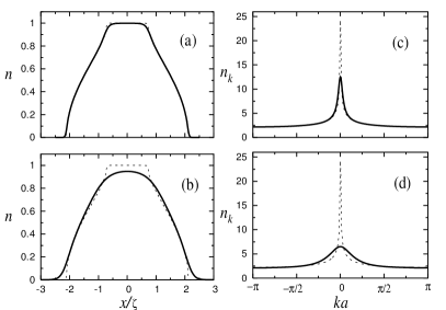
Figure 9: Density (a),(b) and normalized momentum distribution function (d),(d) of 300 HCB’s in a trap with $V_{2}a^{2}=10^{-4}t$ ($\tilde{\rho}=3$) at different temperatures (solid line). The temperature [energy] of the system in each case is $k_{B}T=0.1t$ [$E=158.7t$] (a),(c) and $0.5t$ [$185.9t$] (b),(d). The dashed line in all the figures depicts the ground-state result ($E=157.4t$).

It is worth noticing in Figs. 9(c) and 9(d) that even in the presence of a Mott-insulating phase, at zero temperature, $n_{k}$ exhibits a sharp peak at $k=0$ due to the superfluid phases at the sides wessel04 ; rigol04_1 . The effects of the Mott insulator in $n_{k}$ are reflected by a large population of $k$ states around $ka=\pm\pi$ and an increase of the full width at half maximum of the $k=0$ peak. These are characteristics of the system that remain at finite but very low temperatures. Increasing the temperature [Fig. 9(d)] the peak at $k=0$ disappears. On the other hand, the high-momentum tails remain almost unmodified with respect to the ground-state case as they reflect the properties of short-distance correlations, related to the density profiles, which are much less sensitive to temperature effects.

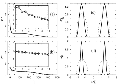
Figure 10: Natural orbital occupations (a),(b) and normalized wave function of the lowest natural orbital (c),(d) for the same systems shown in Fig. 9, $N_{b}=300$ and $V_{2}a^{2}=10^{-4}t$ ($\tilde{\rho}=3$). The temperature [energy] of the system in each case is $k_{B}T=0.1t$ [$E=158.7t$] (a),(c) and $0.5t$ [$185.9t$] (b),(d). The dashed line in all the figures depicts the ground-state result ($T=0$ and $E=157.4$). The insets in (a),(b) display in more detail the lowest 11 natural orbital occupations.

At zero temperature, the natural orbital occupations exhibit a clear signature of the presence of the Mott-insulating core in the trap. A plateau with $\lambda_{\eta}=1$ is present, reflecting the existence of single occupied states. In this case the lowest natural orbital is degenerate due to the splitting of the system by the Mott-insulating core. Two identical quasicondensates can be observed at the sides of the Mott core [Figs. 10(c) and 10(d)]. The increase of temperature reduces the occupation of the lowest natural orbital [they become more localized, Figs. 10(c) and 10(d)], but does not destroy their degeneracy. This degeneracy in absence of a Mott-insulating state is, as explained in the previous subsection, an effect that only appears at finite temperatures due to the population of localized states at the sides of the trap. Finally, one should notice that the plateau with $\lambda_{\eta}=1$ disappears in Fig. 10(b) along with the disappearance of the Mott plateau in Fig. 9(b).

IV.3 Correlation functions and scalings

In Fig. 11 we show the behavior of one-particle correlations with increasing temperature for the two cases analyzed in the previous subsections. Correlations ($\rho_{ij}$) are measured with respect to a fixed point $x_{j}$, while $x_{i}$ is changed all over the system. In Fig. 11(a) the correlations are measured with respect to the middle of the trap and in Fig. 11(b) with respect to two points at the sides of the Mott-insulating core present at $T=0$.

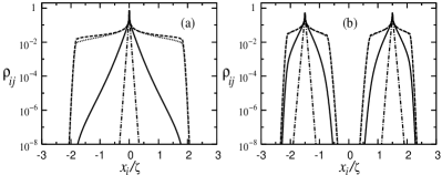
Figure 11: One-particle correlations corresponding to the systems analyzed in Secs. IV.1 and IV.2. (a) $N_{b}=200$, $V_{2}a^{2}=10^{-4}t$ ($\tilde{\rho}=2$), and $x_{j}/\zeta=0$. (b) $N_{b}=300$, $V_{2}a^{2}=10^{-4}t$ ($\tilde{\rho}=3$), and $x_{j}/\zeta=\pm 1.5$. Different temperatures are denoted by $k_{B}T=0$ (dashed line), $0.01t$ (dotted line), $0.10t$ (solid line), and $0.50t$ (dash-dotted line).

In the ground state, the one-particle density matrix decays as a power law $\rho_{ij}\sim|x_{i}-x_{j}|^{-1/2}$ for $0<n_{i},n_{j}<1$ rigol04_1 . The introduction of a small temperature $k_{B}T=0.01t$ can be already noticed in Fig. 11(a) as a faster decay of correlations at long distances. At temperatures larger than $k_{B}T=0.1t$, for the system sizes of the figure, the one-particle density matrix decays exponentially to $10^{-8}$ before reaching the borders of the trap. Due to the space varying density one can notice that in contrast to the box, in a harmonic trap one cannot see a single correlation length, which would mean a straight line in all the semilogarithmic plots of the figure. Still one can calculate the second moment of the one-particle density matrix $\tilde{\xi}$ [Eq. (22)] as a sort of an averaged correlation length.

Table 1: Second moment of the one-particle density matrix ($\tilde{\xi}$), in harmonic traps ($V_{2}a^{2}=10^{-4}t$), for different temperatures, and characteristic densities. We also present values of $\tilde{\xi}$ calculated in boxes ($N=500$) with the same densities than in the center of the trapped case. Notice that in contrast to the characteristic density, the density in the center of the trap changes with increasing temperature. The two values of $\rho$ correspond to $k_{B}T=0.1t$ and $0.5t$, respectively.

$\tilde{\xi}/a$ (trap)	$k_{B}T=0.1t$	$k_{B}T=0.5t$	$\tilde{\xi}/a$ (box)
$\tilde{\rho}=0.5$	8.7 /9.7	1.9 /2.0	$\rho=$0.33,0.29
$\tilde{\rho}=1.0$	10.4 /11.1	2.1 /2.2	$\rho=$0.48,0.47
$\tilde{\rho}=1.5$	10.5 /10.3	2.1 /2.1	$\rho=$0.61,0.61
$\tilde{\rho}=2.0$	9.7 /7.7	2.0 /1.6	$\rho=$0.75,0.75
$\tilde{\rho}=2.5$	8.8 /2.8	1.8 /1.1	$\rho=$0.93,0.87
$\tilde{\rho}=3.0$	8.5 /0.0	1.7 /0.7	$\rho=$1.00,0.95

We present in Table 1 results for $\tilde{\xi}$ in harmonic traps for two temperatures and six values of $\tilde{\rho}$. To the right we show results obtained in boxes with densities chosen to be identical to the ones at the center of the harmonically trapped cloud. One can see that the results in both cases are similar far from the region where the Mott insulator sets in the middle of the trap ($\tilde{\rho}=$0.5–2.0 in Table 1), so that one can estimate $\tilde{\xi}$ in harmonic traps using results from a box. This is in agreement with recent results reported for other finite-temperature correlation lengths in trapped bosonic systems with no lattice kheruntsyan05 . The reason for the agreement between $\tilde{\xi}$ in the trap and in the box is that in the first case $\tilde{\xi}$ is dominated by the contributions of the middle of the system, where the density has its maximum value and it is “relatively uniform.” As one approaches $n=1$ in the middle of the trap, or $\tilde{\rho}=2.6$, the argument above fails ($\tilde{\rho}=2.5,3.0$ in Table 1) since the correlation length in the center of the cloud approaches zero (see $\tilde{\xi}$ vs $\rho$ in Fig. 6 when $\rho\rightarrow 1$) and regions with smaller densities start to dominate the value of $\tilde{\xi}$. For those cases an exact calculation of $\tilde{\xi}$, given the density profile, is required.

Figure 12: Scaling of $n_{k=0}$ (thick lines) and the lowest natural orbital occupation (thin lines) vs $N_{b}$ for a constant characteristic density $\tilde{\rho}=2$. Different temperatures are plotted with the same convention of Fig. 11, $k_{B}T=0$ (dashed line), $0.01t$ (dotted line), $0.05t$ (solid line), and $0.10t$ (dash-dotted line).

The exponential decay of the one-particle density matrix implies that when the size of the system is larger than the averaged correlation length, the momentum distribution function and the occupation of the lowest natural orbital stop changing with increasing system size. The size at which this occurs depends on the temperature, as the averaged correlation length decreases with increasing the temperature, and also depends on the characteristic density. In Fig. 12 we show how $n_{k=0}$ and $\lambda_{0}$ scale at four different temperatures and starting from small system sizes (close to the ones achieved experimentally paredes04 ). At $T=0$ the increase of both quantities is $\sim\sqrt{N_{b}}$, reflecting quasi-long-range correlations present in $\rho_{ij}$ rigol04_1 . For $k_{B}T=0.01t$, the departure from the zero-temperature values occurs when the trap has $\sim 100$ HCB’s. For $k_{B}T=0.05t$ it occurs around $N_{b}=20$, and for $k_{B}T=0.1t$ even the smallest system with 10 HCB’s is different to the ground state.

To conclude this section we show in Fig. 13 a comparison between density and momentum profiles for 100 and 400 HCB’s at $k_{B}T=0.1t$ and $\tilde{\rho}=2$. While even at zero temperature the density profiles do not differ rigol04_1 ; rigol03_3 , the ground-state peak $n_{k=0}$ would have been 2 times larger for 400 HCB’s than for 100 HCB’s. At $k_{B}T=0.1t$ both momentum distribution functions are almost indistinguishable.

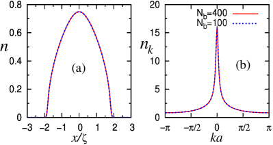
Figure 13: (Color online) Density and momentum profiles in two traps with different filling, but the same $\tilde{\rho}=2$ and $k_{B}T=0.1t$.

V Grand-canonical vs canonical ensemble

In the previous sections we have discussed effects of the temperature on trapped HCB’s in 1D. The starting point for our calculations was the grand-canonical ensemble, in which the system is assumed to be in thermal equilibrium with a large reservoir with temperature $T$ and chemical potential $\mu$. The chemical potential was then chosen to obtain the desired average number of particles in the trap. In this section we analyze the changes introduced by the grand-canonical fluctuations of the particle number with respect to a fixed-$N_{b}$ canonical description, which may be more relevant to describe trapped ultracold quantum gases where no particle reservoir is available.

In the thermodynamic limit both descriptions are known to provide the same predictions huang87 . On the other hand, for noninteracting bosonic systems with a mesoscopic number of particles, it has been shown that the differences between the grand-canonical and canonical condensate fractions can be as large as $10\%$ (for $N_{b}=100$) close to the BEC transition point and decreasing logarithmically with increasing number of particles. In the present work we have been dealing with the opposite case—i.e., infinite repulsion. Interactions are known to suppress fluctuations of the number of particles in the grand-canonical ensemble huang87 , but since recent experiments with HCB’s on optical lattices achieved only up to 20 HCB’s in around 50 lattice sites, it is useful to present an estimate of the difference between both ensembles for such small systems.

In order to obtain the canonical one-particle density matrix we use the ground-state approach of Ref. rigol04_1 . We calculate the Green’s function of all states $|\Psi^{n}_{HCB}\rangle$ with $N_{b}$ bosons in $N$ lattice sites—i.e., of $N_{s}=N!/(N-N_{b})!N_{b}!$ states. The canonical Green’s function at temperature $T$ is obtained as the sum

$$G^{C}_{ij}=\dfrac{1}{Z^{C}}\sum_{n=1}^{N_{s}}e^{-E_{n}/k_{B}T}\langle\Psi^{n}_{HCB}|b_{i}b^{\dagger}_{j}|\Psi^{n}_{HCB}\rangle,$$ (27)

where $e^{-E_{n}/k_{B}T}$ ($E_{n}$ is the energy of state $|\Psi^{n}_{HCB}\rangle$) is the Boltzmann factor and $Z^{C}$ the canonical partition function:

$$Z^{C}=\sum_{n=1}^{N_{s}}e^{-E_{n}/k_{B}T}.$$ (28)

The canonical one-particle density matrix is then

$$\rho^{C}_{ij} = \dfrac{1}{Z^{C}}\sum_{n=1}^{N_{s}}e^{-E_{n}/k_{B}T}\langle\Psi^{n}_{HCB}|b^{\dagger}_{i}b_{j}|\Psi^{n}_{HCB}\rangle$$ (29)

$$= G^{C}_{ij}+\delta_{ij}\left(1-2G^{C}_{ii}\right).$$

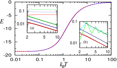
Figure 14: (Color online) Energy (in units of $t$) vs temperature (also in units of $t$) for a box with 50 lattice sites and 10 particles. The grand-canonical ($E$) and canonical ($E^{C}$) results are plotted as solid and dotted lines, respectively. Inset (a) shows $E-E^{C}$ (thin lines) and $\delta E=(E-E^{C})/|E^{C}|$ (thick lines) vs $N_{b}$ for $k_{B}T=0.1t$ (solid line), $0.2t$ (dotted line), $0.5t$ (dashed line). Thin solid lines following $\delta E$ exhibit $1/N_{b}$ behavior. Inset (b) depicts $\delta n_{k}$ for HCB’s and $\delta n^{f}_{k}$ for fermions vs $N_{b}$ (see text). The temperatures are in this case $k_{B}T=0.1t$ (solid line for $\delta n_{k}$, dashed line for $\delta n^{f}_{k}$) and $k_{B}T=0.2t$ (dotted line for $\delta n_{k}$, dash-dotted line for $\delta n^{f}_{k}$). Thin solid lines following these results exhibit $1/N_{b}$ behavior. In both insets the density $\rho=N_{b}/N=0.2$ was kept constant when changing the number of particles.

In Fig. 14 we show results obtained for the grand-canonical ($E$) and canonical ($E^{C}$) energies of 10 HCB’s in a box with 50 lattice sites as a function of the temperature. At the scale of the figure they are indistinguishable. More information can be obtained in the inset (a) where we plot as thin lines the energy difference between both ensembles as a function of the number of particles in boxes with densities $N_{b}/N=0.2$. As seen in this inset even for such small systems the difference almost does not change with $N_{b}$, and it is always smaller than the energy unit $t$. Considering that the modulus of the energy increases linearly with the system size, the relative difference between both ensembles decreases $\delta E\equiv(E-E^{C})/|E^{C}|\sim 1/N_{b}$ [thick lines in inset (a)]. For $N_{b}=10$ and $N=50$ one can see that $\delta E$ is below $1\%$ for temperatures up to $k_{B}T=0.5t$. As the temperature increases beyond $k_{B}T=t$ the differences between $E$ and $E^{C}$ start to decrease, which together with the decrease of the modulus of $E^{C}$ shown in Fig. 14 produces a saturation of $\delta E$ at around $2\%$ for $k_{B}T>10t$. Then for $N_{b}=10$ and $N=50$ the maximum $\delta E$ is just a $2\%$ of the energy. We have also studied other densities keeping $N=50$, and the results obtained for the maximum $\delta E$ were exactly the same $2\%$.

While Kinoshita et al. kinoshita04 used the energy of the system to confirm the achievement of the hard-core limit, Paredes et al. paredes04 considered the momentum distribution function. In the inset (b) of Fig. 14 we show the relative difference [$\delta n_{k}\equiv(\sum_{k}|n_{k}-n^{C}_{k}|)/(\sum_{k}n^{C}_{k})$] between the grand-canonical $n_{k}$ and canonical $n^{C}_{k}$ calculation of the momentum distribution function. The relative differences for $n_{k}$ although larger than the corresponding ones for the energy are still small and also reduce $\sim 1/N_{b}$ with increasing the system size. For $N_{b}=10$ and $N=50$ they are smaller than $1\%$ up to $k_{B}T=0.2t$.

It is also useful to calculate the differences between the grand-canonical and canonical ensemble for the equivalent noninteracting fermions. This may be relevant for systems like the ones recently achieved experimentally by Köhl et al. kohl05 . For noninteracting fermions, the energy differences between both ensembles are identical to the ones of the HCB’s due to the mapping, Eqs. (2)–(5), so that as shown in Fig. 14 and its inset (a) they are small. For the fermionic momentum distribution function the HCB results do not apply. We have also calculated the fermionic relative difference [$\delta n^{f}_{k}\equiv(\sum_{k}|n^{f}_{k}-n^{f,C}_{k}|)/(\sum_{k}n^{f,C}_{k})$] between the grand-canonical $n_{k}^{f}$ and canonical $n^{f,C}_{k}$ calculation of $n_{k}$. They are larger than for the ones of the HCB’s as shown in the inset (b) of Fig. 14. However, they are still small for the experimentally accessible system sizes. For $N_{f}=10$ and $N=50$ they are smaller than $3\%$ for $k_{B}T=0.2t$. Apart from an even-odd effect that decreases with increasing the temperature, $\delta n^{f}_{k}$ also decreases $\sim 1/N_{b}$ with increasing the system size.

The introduction of a harmonic trap does not (qualitatively) change the results obtained in a box. In Fig. 15 we show the grand-canonical and canonical results of the energy in a harmonic trap with 10 particles and $\tilde{\rho}=2$ as a function of the temperature. Contrary to the box, in a harmonic trap the energy is not bounded from above for very large temperatures. This is because the HCB cloud can increase its size and consequently its potential energy. The energy differences between both ensembles, when changing the number of particles keeping $\tilde{\rho}=2$ constant, are shown in the inset of Fig. 15. As for the box they are almost independent of $N_{b}$, and smaller than $t$. The results for the relative differences between the momentum distribution functions for HCB’s and noninteracting fermions in both ensembles are also shown in the inset. Their behavior is very similar to the one of the box in inset (b) of Fig. 14.

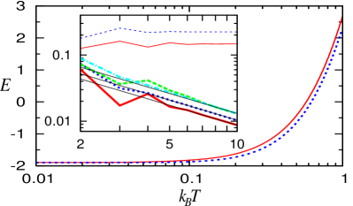
Figure 15: (Color online) Energy vs temperature for a harmonic trap with 10 particles and $\tilde{\rho}=2$. The grand-canonical ($E$) and canonical ($E^{C}$) results are plotted as solid and dotted lines, respectively. The inset shows $E-E^{C}$ (thin lines) and $\delta n_{k}$ (thick lines) vs $N_{b}$ for $k_{B}T=0.3t$ (solid line) and $0.5t$ (dotted line). The $\delta n^{f}_{k}$ of the fermions is also shown as a function of $N_{f}$ (thick lines) for $k_{B}T=0.3t$ (dashed line) and $0.5t$ (dash-dotted line). Thin solid lines following the $\delta n_{k}$ and $\delta n^{f}_{k}$ results exhibit $1/N_{b}$ behavior. In the inset the characteristic density $\tilde{\rho}=2$ was kept constant when changing the number of particles.

As mentioned before, Herzog and Olshanii herzog97 discussed the grand canonical and canonical differences between the condensate fraction for noninteracting bosons in harmonic traps. At finite repulsive interactions, in 1D, there is no BEC even at zero temperature. Still, for the HCB’s we have calculated the differences between the largest eigenvalue of the one-particle density matrix (equivalent to the condensate occupation for BEC leggett01 ) in the grand-canonical and canonical ensembles. As for $\delta n_{k}$ in the inset of Fig. 15, we find that the difference between them decreases $\sim 1/N_{b}$ with increasing number of particles in the system. This clearly contrasts with the $\sim 1/\ln(N_{b})$ obtained for the noninteracting case herzog97 .

We conclude by explicitly showing in Fig. 16 the density profiles and momentum distribution functions of 10 HCB’s in a harmonic trap with $\tilde{\rho}=2$ at $k_{B}T=0.5t$ as obtained from the grand-canonical and canonical descriptions. They are basically indistinguishable. Then, even for the small system sizes achieved experimentally, one can rely on the grand-canonical description for strongly correlated HCB’s for the physical quantities described here. The same conclusion applies to noninteracting fermions.

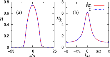
Figure 16: (Color online) Density and momentum profiles of 10 HCB’s in a harmonic trap with $\tilde{\rho}=2$ at $k_{B}T=0.5t$. The grand-canonical and canonical results are plotted as solid and dashed lines respectively.

VI Conclusions

We have presented an exact study of finite-temperature properties of HCB’s confined on 1D lattices. In order to solve this problem we have used the Jordan-Wigner transformation to map HCB’s into noninteracting fermions. After the mapping, properties of Slater determinants allowed us to obtain an exact expression for the HCB one-particle density matrix in terms of determinants of $N\times N$ matrices, which are evaluated numerically. Our approach represents an alternative for finite systems to previous works that considered the thermodynamic limit lieb61 ; mccoy68 ; vaidya78 ; mccoy83 ; tonegawa81 for periodic and open chains and in which Toeplitz determinants were involved.

We have shown that the effects of small finite temperatures are very important when dealing with quantities related to off-diagonal one-particle correlations like the momentum distribution function and the natural orbitals. These finite-temperature effects depend strongly on the system size. On the other hand, observables related to diagonal one-particle correlations (identical for fermions), like density profiles, are much less affected at low temperatures. Explicit results for the behavior of all these quantities versus temperature were given for system sizes that range from the ones recently achieved experimentally up to 20 times larger.

Finally, we have compared grand-canonical and canonical results for energies and momentum distribution functions of HCB’s and noninteracting fermions for small systems, like the ones achieved experimentally. In spite of the mesoscopic number of particles we have shown that for these system sizes the effects of the grand-canonical fluctuations of the particle number are very small and one can rely on a grand-canonical approach.

Although all our calculations are exact for infinite on-site $U$ repulsion, for very strong but finite $U$ our conclusions are still valid. In this case $1/U$ acts like a perturbation to the noninteracting spinless fermion Hamiltonian cazalilla03 . Rey et al. rey05 have recently presented results obtained by exact diagonalization that support the above conclusion rey05 . A connection to experimentally relevant parameters can be also found in Ref. rey05 .

- (1) M. P. A. Fisher, P. B. Weichman, G. Grinstein, and D. S. Fisher, Phys. Rev. B 40, 546 (1989).
- (2) D. Jaksch, C. Bruder, J. I. Cirac, C. W. Gardiner, and P. Zoller, Phys. Rev. Lett. 81, 3108 (1998).
- (3) M. Greiner, O. Mandel, T. Esslinger, T. W. Hänsch, and I. Bloch, Nature (London) 415, 39 (2002).
- (4) S. Wessel, F. Alet, M. Troyer, and G. G. Batrouni, Phys. Rev. A 70, 053615 (2004).
- (5) H. Moritz, T. Stöferle, Michael Köhl, and T. Esslinger, Phys. Rev. Lett. 91, 250402 (2003).
- (6) B. L. Tolra, K. M. O’Hara, J. H. Huckans, W. D. Phillips, S. L. Rolston, and J. V. Porto, Phys. Rev. Lett. 92, 190401 (2004).
- (7) T. Stöferle, H. Moritz, C. Schori, M. Köhl, and T. Esslinger, Phys. Rev. Lett. 92, 130403 (2004).
- (8) G. G. Batrouni, V. Rousseau, R. T. Scalettar, M. Rigol, A. Muramatsu, P. J. H. Denteneer, and M. Troyer, Phys. Rev. Lett. 89, 117203 (2002).
- (9) M. Olshanii, Phys. Rev. Lett. 81, 938 (1998).
- (10) M. Girardeau, J. Math. Phys. 1, 516 (1960).
- (11) E. H. Lieb and W. Liniger, Phys. Rev. 130, 1605 (1963).
- (12) A. Lenard, J. Math. Phys. 5, 930 (1964); 7, 1268 (1966).
- (13) H. G. Vaidya and C. A. Tracy, Phys. Rev. Lett. 42, 3 (1979).
- (14) F. D. M. Haldane, Phys. Rev. Lett. 47, 1840 (1981).
- (15) V. E. Korepin, N. M. Bogoliubov, and A. G. Izergin, Quantum Inverse Scattering Method and Correlation Functions (Cambridge University Press, Cambridge, England, 1993).
- (16) M. A. Cazalilla, J. Phys. B 37, S1 (2004).
- (17) M. D. Girardeau, E. M. Wright, and J. M. Triscari, Phys. Rev. A 63, 033601 (2001).
- (18) P. J. Forrester, N. E. Frankel, T. M. Garoni, and N. S. Witte, Phys. Rev. A 67, 043607 (2003).
- (19) D. M. Gangardt, J. Phys. A 37, 9335 (2004).
- (20) B. Paredes, A. Widera, V. Murg, O. Mandel, S. Fölling, I. Cirac, G. V. Shlyapnikov, T. W. Hänsch, and I. Bloch, Nature (London) 429, 277 (2004).
- (21) T. Kinoshita, T. Wenger, and D. S. Weiss, Science 305, 1125 (2004).
- (22) M. A. Cazalilla, Phys. Rev. A 70, 041604(R) (2004).
- (23) E. Lieb, T. Shultz, and D. Mattis, Ann. Phys. (N.Y.) 16, 407 (1961).
- (24) B. M. McCoy, Phys. Rev. 173, 531 (1968).
- (25) H. G. Vaidya and C. A. Tracy, Phys. Lett. A 68, 378 (1978).
- (26) B. M. McCoy, J. H. Perk, and R. E. Schrock, Nucl. Phys. B 220, 35 (1983); 220, 269 (1983).
- (27) M. Rigol and A. Muramatsu, Phys. Rev. A 70, 031603(R) (2004); 72, 013604 (2005).
- (28) M. Rigol and A. Muramatsu, Phys. Rev. Lett. 93, 230404 (2004).
- (29) M. Rigol and A. Muramatsu, Phys. Rev. Lett. 94, 240403 (2005).
- (30) O. Penrose and L. Onsager, Phys. Rev. 104, 576 (1956).
- (31) A. J. Leggett, Rev. Mod. Phys. 73, 307 (2001).
- (32) P. Jordan and E. Wigner, Z. Phys. 47, 631 (1928).
- (33) A. Muramatsu, in Quantum Monte Carlo Methods in Physics and Chemistry, Vol. 525 of NATO Advanced Studies Institute, Series C: Mathematical and Physical Sciences, edited by M. P. Nightingale and C. J. Umrigar, (Kluwer Academic, Dordrecht, 1999), pp. 343–373.
- (34) F. F. Assaad, in Quantum Simulations of Complex Many-Body Systems: From Theory to Algorithms, edited by J. Grotendorst, D. Marx, and A. Muramatsu (John von Neumann Institute for Computing, Jülich, 2002), Vol. 10, pp. 99–155.
- (35) T. Tonegawa, Solid State Commun. 40, 983 (1981).
- (36) M. Rigol and A. Muramatsu, Phys. Rev. A 70, 043627 (2004).
- (37) C. Hooley and J. Quintanilla, Phys. Rev. Lett. 93, 080404 (2004).
- (38) V. Ruuska and P. Törmä, New J. Phys. 6, 59 (2004).
- (39) A. M. Rey, G. Pupillo, C. W. Clark, and C. J. Williams, Phys. Rev. A 72, 033616 (2005).
- (40) Or what is the same, for energies exceeding in (which is the bandwidth in 1D) the energy of the lowest eigenstate of the Hamiltonian rigol03_3 .
- (41) K. V. Kheruntsyan, D. M. Gangardt, P. D. Drummond, and G. V. Shlyapnikov, Phys. Rev. A 71, 053615 (2005).
- (42) K. Huang, Statistical Mechanics, 2nd ed. (Wiley, New York, 1987).
- (43) C. Herzog and M. Olshanii, Phys. Rev. A 55, 3254 (1997).
- (44) M. Köhl, H. Moritz, T. Stöferle, K. Günter, and T. Esslinger, Phys. Rev. Lett. 94, 080403 (2005).
- (45) M. A. Cazalilla, Phys. Rev. A 67, 053606 (2003).