The Average Shape of Transport-Limited Aggregates

Abstract

We study the relation between stochastic and continuous transport-limited growth models, which generalize conformal-mapping formulations of diffusion-limited aggregation (DLA) and viscous fingering, respectively. We derive a nonlinear integro-differential equation for the asymptotic shape (average conformal map) of stochastic aggregates, whose mean-field approximation is the corresponding continuous equation, where the interface moves at its local expected velocity. Our equation accurately describes advection-diffusion-limited aggregation (ADLA), and, due to nonlinear averaging over fluctuations, the average ADLA cluster is similar, but not identical, to an exact solution of the mean-field dynamics. Similar results should apply to all models in our class, thus explaining the known discrepancies between average DLA clusters and viscous fingers in a channel geometry.

Developing effective mean field approximations to nonlinear stochastic equations constitutes a major challenge in various active fields of statistical physics, e.g. hydrodynamic turbulence Frisch and self organized criticality Bak . Straightforward derivation of such approximate theories typically involves uncontrolled assumptions required to ”close” an infinite hierarchy of equations for moments of the probability distribution of the stochastic field. An alternative approach consists of deriving asymptotic solutions to a deterministic version of the original stochastic dynamics, assuming that such solutions capture the behavior of ensemble average of the original stochastic field Bak . Such approach, however, might turn out to be unreliable as well, since it underestimates the possible effects of noise on the asymptotic evolution of a stochastic field.

A nontrivial example in which such approach has been advanced over the last two decades is the fractal morphology of patterns observed in computer simulations of the celebrated diffusion limited aggregation (DLA) model witten81 . Since the relation between the mathematical formulations of the stochastic DLA process and the continuous viscous fingering dynamics was established Paterson84 , the striking similarity between patterns observed in both processes has triggered various attempts to interpret viscous fingering dynamics as a mean field for DLA stanley91 ; arneodo89 ; barra02 ; swinney03 .

In this Letter, we study the connection between a broad class of stochastic transport-limited aggregation processes and their continuous counterparts bazant03 . In our models, growth is fuelled by nonlinear, non-Laplacian transport processes, such as advection-diffusion and electrochemical conduction, which satisfy conformally invariant equations bazant04 . Stochastic and continuous dynamics are defined by generalizing conformal-mapping formulations of DLA hastings98 and viscous fingering polubarinova45 ; shraiman84 , respectively. We show that the continuous dynamics is a self-consistent mean-field approximation of the stochastic dynamics, which, nevertheless, does not accurately predict the average shape of a random ensemble of aggregates.

(a)

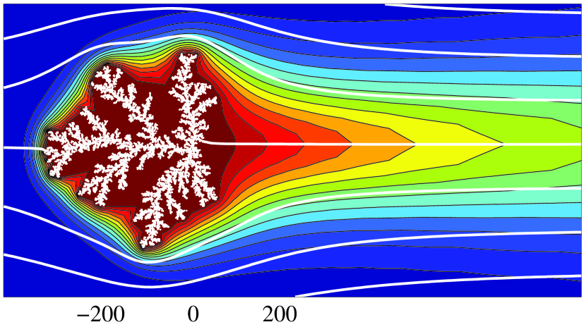
(b)

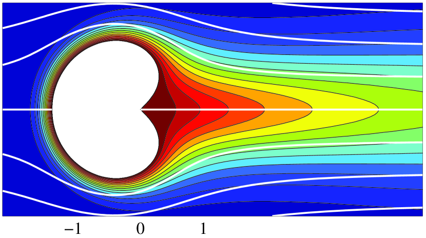
Figure 1: (a) A typical ADLA cluster of $n=10^{5}$ “particles” (iterated conformal maps). Color contours indicate the particle concentration $c$, and solid yellow curves are fluid streamlines. (b) The exact, asymptotic shape of the analogous continuous dynamics, $G_{c}(w)$, which describes solidification in a fluid flow. For both (a) and (b), we set $\mathrm{Pe}\approx 20$ so that the far fields are similar.

We consider a set of two-dimensional scalar fields, $\boldsymbol{\varphi}=\{\varphi_{1},\varphi_{2},\ldots,\varphi_{M}\}$, whose gradients produce quasi-static, conserved “flux densities”,

$$\mathbf{F}_{i}=\sum_{j=1}^{M}C_{ij}(\boldsymbol{\varphi})\boldsymbol{\nabla}\varphi_{j}\;,\qquad\boldsymbol{\nabla}\cdot\mathbf{F}_{i}=0$$ (1)

in $\Omega_{z}(t)$, the exterior of a singly connected domain that represents a growing aggregate at time $t$. (The coefficients, $\{C_{ij}\}$ may be nonlinear functions of the fields.) The crucial property of the nonlinear system (1) is its conformal invariance bazant04 : If $\boldsymbol{\varphi}(w,\overline{w})$, not necessarily harmonic, is a solution in a domain $\Omega_{w}$ and $w=f(z)$ is a conformal map from $\Omega_{z}$ to $\Omega_{w}$, then $\boldsymbol{\varphi}(f(z),\overline{f(z)})$ is a solution in $\Omega_{z}$. Using this fact, the evolving domain, $\Omega_{z}(t)$, can be described by the conformal map, $z=g(w,t)$, from the exterior of (say) the unit disk, $\Omega_{w}$.

Growth is driven by a combination of flux densities, $\mathbf{Q}=\sum_{i=1}^{N}B_{i}(\boldsymbol{\varphi})\mathbf{F}_{i}$, on the boundary with a local growth rate, $\sigma=\mbox{\boldmath{$\hat{n}$}}\cdot\mathbf{Q}$, where $\boldsymbol{\hat{n}}$ is the unit normal vector at $z\in\partial\Omega_{z}(t)$. For continuous, deterministic growth, each boundary point $z$ moves with a velocity, $\boldsymbol{v}(z)=\alpha\,\sigma(z)\,\mbox{\boldmath{$\hat{n}$}}(z)$, where $\alpha$ is a constant. For discrete, stochastic growth, the initial seed, $\Omega_{z}(t_{0}=0)$, is iteratively advanced by elementary “bump” maps representing particles of area $\lambda_{0}$ at times $t_{1},\cdots,t_{n}$. The waiting time $t_{n}-t_{n-1}$ is an exponential random variable with a mean set by the total integrated flux. The probability density to add the $n$th particle in a boundary element $(z,z+dz)\in\partial\Omega_{z}(t_{n-1})$ is proportional to $\sigma(z)|dz|$.

The classical models are recovered in the simplest case of one field ($M=1$). DLA corresponds to stochastic growth by diffusion, $\mathbf{F}=\mathbf{Q}=-D\boldsymbol{\nabla}c$, from a distant source ($c\sim\log|z|$ as $|z|\to\infty$) to an absorbing cluster ($c=0$ for $z\in\Omega_{z}(t)$), where $c$ is the particle concentration and $D$ the diffusivity. Viscous fingering corresponds to continuous growth by the same process, where $c$ becomes the fluid pressure and $D$ the permeability.

The simplest, nontrivial models with multiple fields ($M=2$) involve diffusion in a fluid flow. The stochastic case is advection-diffusion-limited aggregation (ADLA) bazant03 , illustrated in Fig. 1a. Particles are deposited around a circular seed of radius, $L_{o}$, from potential flow, $\boldsymbol{v}=\nabla\varphi$, of uniform velocity $U$ far from the aggregate. The dimensionless transport problem is

$$\mathrm{Pe}_{o}\boldsymbol{\nabla}\varphi\cdot\boldsymbol{\nabla}c=\boldsymbol{\nabla}^{2}c,\quad\boldsymbol{\nabla}^{2}\varphi=0,\quad z\in\Omega_{z}(t)$$ (2)

$$c=0,\quad\mbox{\boldmath{$\hat{n}$}}\cdot\boldsymbol{\nabla}\varphi=0,\quad\sigma=\mbox{\boldmath{$\hat{n}$}}\cdot\boldsymbol{\nabla}c,\quad z\in\partial\Omega_{z}(t)$$ (3)

$$c\to 1,\quad\boldsymbol{\nabla}\varphi\to\mbox{\boldmath{$\hat{x}$}},\quad|z|\to\infty,$$ (4)

where $c$ is the concentration of particles. Here $x$, $\varphi$, $c$, and $\sigma$ are in units of $L_{o}$, $UL_{o}$, $C$, and $DC/L_{o}$, respectively, and $\mathrm{Pe}_{o}=UL_{o}/D$ is the initial Péclet number. Numerical solutions and asymptotic approximations are discussed in Ref. choi04 .

The transport problem is conformally invariant, except for the boundary condition, Eq. (4), which alters the flow speed upon conformal mapping. Instead, we choose to fix the mapped background flow and replace $\mathrm{Pe}_{o}$ with the renormalized Péclet number, $\mathrm{Pe}(t)=A_{1}(t)\mathrm{Pe}_{o}$, when Eq. (2) is transformed from $\Omega_{z}(t)$ to $\Omega_{w}$. The “conformal radius”, $A_{1}(t)$, is the coefficient of $w$ in the Laurent expansion of $g(w,t)$ and scales with the radius of the growing object hastings98 ; davidovitch99 . Since $A_{1}(t)\rightarrow\infty$ for any initial condition, the flux approaches a self-similar form,

$$\sigma(\theta;\mathrm{Pe})\sim 2\sqrt{\mathrm{Pe}/\pi}\;\sin(\theta/2)\quad\text{as}\quad\mathrm{Pe}\to\infty.$$ (5)

More generally, there is a universal crossover from DLA ($\sigma=$ constant) to this stable fixed point, where $\mathrm{Pe}(t)=A_{1}(t)\mathrm{Pe}_{o}$ is the appropriate scaling variable choi05 .

The continuous analog of ADLA is a simple model for solidification from a flowing melt kornev94 . More generally, continuous dynamics in our class is described by a nonlinear equation,

$$\mathrm{Re}\,(\overline{w\,g^{\prime}}\;g_{t})=\alpha\;\sigma(w;\mathrm{Pe}(t))\quad\text{for}\quad|w|=1.$$ (6)

which generalizes the Polubarinova-Galin equation for Laplacian growth polubarinova45 ; shraiman84 ($\sigma=1$). In the case of advection-diffusion kornev94 , only low-$\mathrm{Pe}$ approximations are known, but we have found an exact high-$\mathrm{Pe}$ solution of the form, $g(w,t)=A_{1}(t)\,G_{c}(w)$, where

$$A_{1}(t)=t^{2/3},\quad G_{c}(w)=w\,\sqrt{1-1/w}.$$ (7)

This similarity solution to Eq. (6) with $\alpha\,\sigma(\theta,t)=\sqrt{A_{1}(t)}\sin(\theta/2)$ describes the long-time limit, according to Eq. (5). (We do not know the uniqueness or stability of this solution or whether it can be approached without singularities from general initial conditions.) Just as the Saffman-Taylor finger solution (for $\sigma=1$) has been compared to DLA in a channel geometry somfai_ball02 , this analytical result begs comparison with ADLA.

As in Ref. bazant03 , we grow ADLA clusters by a modified Hastings-Levitov algorithm hastings98 . The random attachment of the $n$th particle to the cluster is described by perturbing the boundary $\partial\Omega_{z}(t_{n-1})\to\partial\Omega_{z}(t_{n})$ by a “bump” of characteristic area $\lambda_{0}$. This leads to the recursive dynamics

$$g_{n}(w)=g_{n-1}\circ\phi_{\lambda_{n},\theta_{n}}(w),\quad g_{n}(w)=g(w,t_{n})$$ (8)

where $\phi_{\lambda,\theta}(w)$ is a specific map, conformal in $\Omega_{w}$, that slightly distorts the unit circle by a bump of area $\lambda$ around the angle $\theta$. The parameter, $\lambda_{n}=\lambda_{0}|g_{n-1}^{\prime}(e^{i\theta_{n}})|^{-2}$ is the area of the pre-image of such bump under the inverse map $g^{-1}$. The angle $\theta_{n}$ is chosen with a probability density $p(\theta;\mathrm{Pe}(t_{n}))\propto\sigma(e^{i\theta};\mathrm{Pe}(t_{n}))$, so the expected growth rate is the same as in the continuous dynamics.

For an ensemble of $n$-particle aggregates, a natural definition of average cluster shape is the conformal map, $\langle{G_{n}(w)}\rangle$, defined by averaging at a point $w\in\Omega_{w}$ all the maps, $G_{n}(w)=g_{n}(w)/A_{1}(t_{n})$, rescaled to have a unit conformal radius. We then ask: What is the limiting average cluster shape, $\langle{G_{\infty}(w)}\rangle=\lim_{n\to\infty}\langle{G_{n}(w)}\rangle$, and how does it compare to the similarity solution, $G_{c}(w)$, of the continuous growth equation (6)? The same questions apply to any of our transport-limited growth models, but here we focus on ADLA as a representative case.

To provide numerical evidence, we grow 2000 ADLA clusters of size $n=10^{5}$ using the semi-circular bump function in Ref. davidovitch99 (with $a=1/2$). To reduce fluctuations, we aggregate small particles, $\lambda_{0}=1/16$, on a large initial seed ($g_{0}(w)=w,|w|=1$). To reach at the asymptotic limit faster and also match the assumption of $G_{c}(w)$, we fix the angular probability measure, $p_{\infty}(\theta)=\sin(\theta/2)/4$ for $\mathrm{Pe}=\infty$, throughout the growth. In Fig. 2a, we plot the average contour of the ensemble, $\langle{G_{n}(e^{i\theta})}\rangle$ at $n=10^{5}$ along with that of the continuous solution, $G_{c}(e^{i\theta})$. To give a sense of fluctuations, we also plot a “cloud” of points, $G_{n}(e^{i\theta})$ over uniformly sampled values of $\theta$. Fig. 2b is the zoom-in of the boxed region in Fig. 2a, where we also show $\langle{G_{n}(e^{i\theta})}\rangle$ at $n=10^{3}$ and $n=10^{4}$. Although the convergence of $\langle{G_{n}(w)}\rangle$ is easily extrapolated, the $n=10^{5}$ line has not reached at the asymptotic limit yet. The branch point at $w=1$ seems to be related to the slow convergence. Ignoring the unconverged area, $\langle{G_{n}(w)}\rangle$ and $G_{c}(w)$ are quite similar, and yet clearly not same. The average, $\langle{G_{n}(w)}\rangle$, better captures the ensemble morphology reflected by the cloud pattern than $G_{c}(w)$ and the opening angles at the branch point of the two curves are also different choi05 .

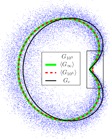
(a) (b)

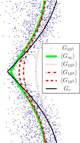
Figure 2: (a) The “cloud” of the sampled points, $G_{n}(e^{i\theta})$ and its mean field contour, $\langle{G_{n}(e^{i\theta})}\rangle$ at $n=10^{5}$ (dashed) displayed with the asymptotic limit, $\langle{G_{\infty}(e^{i\theta})}\rangle$ and the steady state shape of the continuous growth, $G_{c}(e^{i\theta})$. (b) The zoom-in of the box in (a). Two contours, $\langle{G_{n}(e^{i\theta})}\rangle$, at $n=10^{3}$ (dotted) and $10^{4}$ (dashed dot) are added to show the slow convergence to $\langle{G_{\infty}(e^{i\theta})}\rangle$ near the rear stagnation point.

Next we derive an equation for $\langle{G_{n}(w)}\rangle$ in the asymptotic regime. For growing aggregates $\lambda_{n}\to 0$ as $n\to\infty$ davidovitch99 . Following Hastings hastings97 , we use Eq. (8) to derive a linearized recursive equation for $G_{n+1}(w)$ for $|w-e^{i\theta_{n+1}}|\gg\sqrt{\lambda_{n+1}}$. Letting $(\lambda,\theta)$ denote the parameters of the $(n+1)$th bump, we obtain:

$$G_{n+1} (w)\sim(1-a\lambda)(G_{n}(w)+a\lambda H_{\theta}(w)G_{n}^{\prime}(w))$$ (9)

$$\sim G_{n}(w)+a\lambda(H_{\theta}(w)G_{n}^{\prime}(w)-G_{n}(w)).$$

where $H_{\theta}(w)=w\,(w+e^{i\theta})\,/\,(w-e^{i\theta})$ and we use $A_{1}(t_{n+1})=(1+\lambda)^{a}\;A_{1}(t_{n})$.

Stationarity of the ensemble of rescaled clusters implies:

$$\langle{G_{n}(w)}\rangle=\int_{0}^{2\pi}d{\theta}\;p_{\infty}(\theta)\langle{G_{n+1}(w)}\rangle\ .$$ (10)

Our analysis applies for conformally invariant transport-limited growth from an isolated seed with general angular probability distributions, although we will focus on the case of ADLA, $p_{\infty}(\theta)=\sin(\theta/2)/4$.

Using Eq. (9), we get the fixed-point condition:

$$\int_{0}^{2\pi}d{\theta}\;\,p_{\infty}(\theta)\langle{\lambda G_{\infty}(w)}\rangle\sim\int_{0}^{2\pi}d{\theta}\;\,p_{\infty}(\theta)\langle{\lambda G_{\infty}^{\prime}(w)}\rangle H_{\theta}(w).$$ (11)

To facilitate further analysis, we approximate the left hand side of Eq. (11) as

$$\int_{0}^{2\pi}d{\theta}\;p_{\infty}\langle{\lambda G_{\infty}}\rangle\approx\int_{0}^{2\pi}d{\theta}\;p_{\infty}\langle{\lambda}\rangle\langle{G_{\infty}}\rangle$$ (12)

and the right hand side similarly. We checked the validity of this assumption by numerical evaluation of these two quantities for increasing values of $n$, finding less than 1% discrepancy for the largest clusters ($n=10^{5}$). Although the stronger assumption, $\langle{\lambda G_{\infty}}\rangle\approx\langle{\lambda}\rangle\langle{G_{\infty}}\rangle$, is not valid, particularly near the bump center $w=e^{i\theta}$, the correlation seems to be canceled out in the integration along the angle.

With these assumptions, we arrive at a nonlinear integro-differential equation for $\langle{G_{\infty}(w)}\rangle$, the limiting average cluster shape:

$$\frac{\langle{G_{\infty}(w)}\rangle}{\langle{G_{\infty}(w)}\rangle^{\prime}} =\frac{\int_{0}^{2\pi}d{\theta}\;\,p_{\infty}(\theta)\,\langle{|G_{\infty}^{\prime}(e^{i\theta})|^{-2}}\rangle\,H_{\theta}(w)}{\int_{0}^{2\pi}d{\theta}\;\,p_{\infty}(\theta)\,\langle{|G_{\infty}^{\prime}(e^{i\theta})|^{-2}}\rangle}$$ (13)

$$=\int_{0}^{2\pi}d{\theta}\;\,p_{\infty}(\theta)\,\Lambda_{\infty}(\theta)\,H_{\theta}(w)$$ (14)

where we introduce a conditional probability density,

$$\Lambda_{n}(\theta)=\frac{\langle{|G_{n}^{\prime}(e^{i\theta})|^{-2}}\rangle}{\int_{0}^{2\pi}d{\theta^{\prime}}\;p_{\infty}(\theta^{\prime})\,\langle{|G_{n}^{\prime}(e^{i\theta^{\prime}})|^{-2}}\rangle},$$ (15)

proportional to the average local size of a bump’s pre-image (Jacobian factor), $\langle{\lambda_{n}}\rangle$, at angle $\theta$. In deriving Eq.  (13) we assume that $\langle{A_{1}(t_{n})|G_{n}^{\prime}|^{-2}}\rangle\sim\langle{A_{1}(t_{n})}\rangle\langle{|G_{n}^{\prime}|^{-2}}\rangle$ as $n\to\infty$ choi05 . The stochastic nature of the aggregates is manifested through the two different averages in Eqs. (14)–(15).

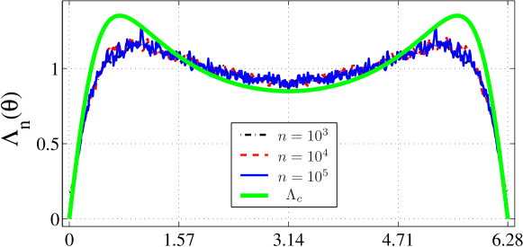
Figure 3: The angular profile of the Jacobian factor, $\Lambda_{n}(\theta)$, which shows how the size of bump pre-images varies on the unit circle, at three stages of growth in simulations: $n=10^{3}$ (dashed), $n=10^{4}$ (dash-dot) and $n=10^{5}$ (solid). The exact mean-field approximation, $\Lambda_{c}(\theta)$, (thick gray) obtain from Eq. (7) shows a clear difference with $\Lambda_{n}(\theta)$.

To check the validity of Eq. (14), we obtain $\Lambda_{\infty}$ from simulations and solve for $\langle{G_{\infty}(w)}\rangle$. As shown in Fig. 3, the measured curves for $\Lambda_{n}(\theta)$ for $n=10^{3},\,10^{4}$ and $10^{5}$ are nearly identical, so we conclude that $\Lambda_{10^{5}}(\theta)$ is a good approximation of $\Lambda_{\infty}(\theta)$. Now we solve Eq. (14) by expanding $\langle{G_{\infty}(w)}\rangle$ by a Laurent series and finding recurrence relations for the coefficients, which involve integrals of $\Lambda_{\infty}(\theta)$. We calculate 200 first coefficients and reconstruct $\langle{G_{\infty}(w)}\rangle$. The image of the unit circle under $\langle{G_{\infty}(w)}\rangle$, shown in Fig.2a (thick gray), is in excellent agreement with the converging pattern of $\langle{G_{n}(w)}\rangle$.

The surprising difference between the convergence rates of the average Jacobian $\Lambda_{n}(\theta)$ and the average map itself $\langle{G_{n}(w)}\rangle$ is intimately related to the multifractal nature of the distribution of the stretching factor (harmonic measure) $|G_{n}^{\prime}(e^{i\theta})|$. Since this factor is very large around the cusp at $\theta=0$, which is dominant during the growth process, fluctuations at the cusp do not contribute to negative moments of the distribution of $|G_{n}^{\prime}(e^{i\theta})|$ and thus negative moments converge much faster than positive ones, and faster than the average map itself. Since $\Lambda_{n}(\theta)$ comes from averaging $|G_{n}^{\prime}(e^{i\theta})|^{-2}$, this observation explains its fast convergence. This argument illustrates how the two averages interact in Eqs. (14)–(15) and suggests that the faster convergence of $\Lambda_{n}(\theta)$ dominates the morphology.

With the validity of Eq. (14) established, we may consider its mean-field version, where the ensemble average is replaced by a single conformal map, given by:

$$\frac{G_{c}(w)}{G_{c}^{\prime}(w)}=\int_{0}^{2\pi}d{\theta}\;p_{\infty}(\theta)\,\Lambda_{c}(\theta)\,H_{\theta}(w),$$ (16)

$$\Lambda_{c}(\theta)=\frac{|G_{c}^{\prime}(e^{i\theta})|^{-2}}{\int_{0}^{2\pi}d{\tilde{\theta}}\;p_{\infty}(\tilde{\theta})\,|G_{c}^{\prime}(e^{i\tilde{\theta}})|^{-2}}.$$ (17)

Not surprisingly, the similarity solution for continuous growth, Eq. (7), is an exact solution of Eqs. (16)–(17). In fact, it is possible to derive Eqs. (16)–(17) from a different representation of Eq. (6), which has been done for the case of DLA, $p_{\infty}(\theta)=1/2\pi$, in Ref. hastings97 . Elsewhere choi05 , we obtain an analytical form for $\Lambda_{c}(\theta)$ for ADLA, which is plotted in Fig. 3 (thick gray). A small, but significant, difference between $\Lambda_{c}(\theta)$ and $\Lambda_{\infty}(\theta)$ is apparent, especially at $\theta=\pi/4$ and $7\pi/4$.

The solution in Eq. (7) can be interpreted as a self-consistent mean-field approximation for the average conformal map, $\langle{G_{\infty}(w)}\rangle$. However, fluctuations in the ensemble manifest themselves through the different averages in Eqs. (14)–(15). As long as $\langle{|G_{\infty}^{\prime}(w)|^{-2}}\rangle$ is different from $|\langle{G_{\infty}(w)}\rangle^{\prime}|^{-2}$, $\Lambda_{\infty}(\theta)\neq\Lambda_{c}(\theta)$, and thus the deviation of $\langle{G_{\infty}(w)}\rangle$ from $G_{c}(w)$ is inevitable.

We believe that the assumptions leading to Eq. (14) are quite general, and not specific to ADLA, so the continuous dynamics should be a mean field theory (in this sense) for any stochastic aggregation, driven by conformally invariant transport processes, Eq. (1). We conclude, therefore, that the solution to the continuous dynamics, although similar, is not identical to the ensemble-averaged cluster shape. An exceptional case is DLA in radial geometry, where isotropy implies the trivial solution, $\langle{G_{\infty}(w)}\rangle=w$ and $\Lambda_{c}(\theta)=1$. Clearly, $G_{c}(w)=w$ and $\Lambda_{c}(\theta)=1$ solves Eq. (14) with $p_{\infty}(\theta)=1/2\pi$.

We expect, however, that this identity between the mean-field approximation and the average shape of stochastic clusters will be removed with any symmetry breaking, either in the model equations (such as ADLA) or in the BCs (e.g. DLA in a channel). This result is consistent with recent simulations of DLA in a channel geometry somfai_ball02 , which show that the average cluster shape, $\langle{G_{n}(w)}\rangle$, is similar, but not identical, to any of the Saffman-Taylor “fingers”, which solve the continuous dynamics. We expect that an analogous equation to Eq. (14), relating $\langle{G_{\infty}(w)}\rangle$ and $\langle{|G_{\infty}^{\prime}(e^{i\theta})|^{-2}}\rangle$, will hold in a channel geometry, and Saffman-Taylor fingers should be exact solutions to the mean-field approximation of that equation.

We conclude by emphasizing that, although Eq. (14) is a necessary condition for the average shape of transport-limited aggregates in the class, Eq. (1), it does not provide a basis for complete statistical theory. Such a theory would likely consist of an infinite set of independent equations connecting a hierarchy of moments of the multifractal distributions of maps $\{G_{\infty}(w)\}$, and derivatives $\{G_{\infty}^{\prime}(w)\}$. Multifractality may speed up convergence, as for Eq. (14), or slow down convergence of other equations in this set. The mean-field approximation, Eq. (16), which corresponds to the continuous growth process, can be considered as leading a hierarchy of closure approximations to this set.

This work was supported in part by the MRSEC program of the National Science Foundation under Award No. DMR 02-13282 (M.Z.B), and by Harvard MRSEC (B.D).

References

- (1) U. Frisch, Turbulence: The Legacy of A.N. Kolmogorov, (Cambridge University Press, Cambridge, 1995).
- (2) P. Bak, How Nature Works: The Science of Self-Organized Criticality, (Springer-Verlag, Telos, 1999).
- (3) T. A. Witten and L. M. Sander, Phys. Rev. Lett. 47, 1400 (1981).
- (4) L. Paterson, Phys. Rev. Lett. 52, 1621 (1984).
- (5) H.E. Stanley, in ”Fractals and Disordered Systems”, A. Bunde and S. Havlin (Eds.), Springer-Verlag (1991).
- (6) A. Arneodo, Y. Couder, G. Grasseau V. Hakim and M. Rabaud, Phys. Rev. Lett. 63, 984 (1989).
- (7) F. Barra, B. Davidovitch and I. Procaccia, Phys. Rev. E. 65, 046144 (2002).
- (8) E. Sharon, M. G. Moore, W. D. McCormick and H. L. Swinney, Phys. Rev. Lett. 91, 205504 (2003).
- (9) M. Z. Bazant, J. Choi, and B. Davidovitch, Phys. Rev. Lett. 91, 045503 (2003)
- (10) M. Z. Bazant, Proc. R. Soc. Lond. A, 460, 1433 (2004)
- (11) M. Hastings and L. Levitov, Physica D 116, 244 (1998).
- (12) P. Ya. Polubarinova-Kochina, Dokl. Akad. Nauk. S. S. S. R. 47, 254 (1945); L. A. Galin, 47, 246 (1945).
- (13) B. Shraiman and D. Bensimon, Phys. Rev. A, 30, 2840 (1984).
- (14) J. Choi, D. Margetis, T. M. Squires, and M. Z. Bazant, To appear in J. Fluid Mech.
- (15) B. Davidovitch, H. G. E Hentschel, Z. Olami, I. Procaccia, L. M. Sander, and E. Somfai, Phys. Rev. E 59, 1368 (1999).
- (16) J. Choi, M. Z. Bazant, and B. Davidovitch, in preparation.
- (17) K. Kornev, K. and G. Mukhamadullina, Proc. Roy. Soc. London A 447, 281–297 (1994).
- (18) E. Somfai R. C. Ball, J. P. DeVita and L. M. Sander, Phys. Rev. E 68, 020401 (2003).
- (19) M. B. Hastings, Phys. Rev. E 55, 135 (1997).