Hybrid Burnett Equations.
A New Method of Stabilizing

Abstract

In the original work by Burnett the pressure tensor and the heat current contain two time derivates. Those are commonly replaced by spatial derivatives using the equations to zero order in the Knudsen number. The resulting conventional Burnett equations were shown by Bobylev to be linearly unstable. In this paper it is shown that the original equations of Burnett have a singularity. A hybrid of the original and conventional equations is constructed which is shown to be linearly stable. It contains two parameters. For the simplest choice of parameters the hybrid equations have no third derivative of the temperature but the inertia term contains second spatial derivatives. For stationary flow, when terms $K\!n^{2}M\!a^{2}$ can be neglected, the only difference from the conventional Burnett equations is the change of coefficients $\varpi_{2}\rightarrow\varpi_{3},\varpi_{3}\rightarrow\varpi_{3}.$

I Introduction

The practical interest of extending the Navier-Stokes equations to smaller length scales comes from the need to model re-entrance of space vehicles and in later times from nano scale technology. In this parameter region there is in general the Boltzmann equation. As the collision integral is very heavy to calculate numerically, the Boltzmann equation is usually applied for fairly simple or idealized problems, see Cercignani Cercignanis lilla bok . An other method is that of DSMC due to Bird Bird . But in the collision dominated region also DSMC is very demanding computationally. Hence special methods are valuable when the Knudsen number is too large for the Navier-Stokes equations to apply but still small enough to allow for an expansion. A fruitful technique in this region is the asymptotic method, originating with Hilbert and Grad, see Sone Sone .

The Navier-Stokes equations were derived from the Boltzmann equation by the Chapman-Enskog method, see Chapman & Cowling CC . They are to first order in the mean free path. The corresponding equations to second order in the mean free path were derived by Burnett Burnett , see also CC . However, the Burnett equations were proven by Bobylev Bobylev to have a nonphysical instability. See also the review by Agarwal et al Agarwal and the paper by Uribe et al. Uribe .

For the Burnett equations the trivial state of rest is thus unstable for perturbations of a wavelength of the order of the mean free path and shorter. The Chapman-Enskog method is an expansion in the Knudsen number $K\!n=l/L$, where $l$ is the mean free path and $L$ a characteristic length. Wavelengths of the order of the mean free path and larger correspond to an effective Knudsen number of the order $1$ and larger. So there is no contradiction in the fact that the Burnett equations are unstable for short wavelengths. The physical content of the Burnett equations is for solutions with a characteristic length which is large enough. But nevertheless the equations should be wellbehaved for all length scales. This is necessary mathematically as well as numerically.

As pointed out by Agarwal et al Agarwal Burnett’s original expression for the viscous pressure tensor contains the time derivative of the traceless rate of deformation tensor. Chapman & Cowling replace the time derivative by spatial derivatives using the equations at the Euler level. Agarwal et al give the name conventional Burnett equations to the resulting equations. There is a similar replacement for the time derivative of the temperature gradient. This method of replacement using the zero order equations is part of the procedure in the Chapman-Enskog method to obtain the Navier-Stokes equations from the Boltzmann equation to first order of the Knudsen number.

Agarwal et al also raise the question if the instability of the conventional Burnett equations is caused by this replacement, so that possibly the original Burnett equations are linearly stable. In the present paper we show that the original Burnett equations have an unphysical singularity. In Jin Jin and Slemrod introduce $\mathbf{P,q}$ as new independent fields and propose 13 equations, first order in time and second order in space. See also the two master theses by Svärd Svard and by Strömgren Stromgren and the paper by Söderholm Soderholm based on essentially the same idea but with equations which are first order in time as well as space. In the paper Soderholm these equations are applied numerically for nonlinear sound waves.

In the present paper we introduce a two parameter partial replacement of the mentioned time derivatives and show that the parameters can be chosen to give linear stability. We then choose the parameters such that the resulting equations are as close to the original and conventional equations as possible. The resulting equations are more similar to the already studied Burnett equations than those in Jin and Soderholm and it seems that it should be simpler to reduce a numerical scheme for the equations to one for the Navier-Stokes equations.

II The Burnett Equations

The general equations of balance are

$$\frac{D\rho}{Dt}+\rho\mathbf{\nabla\cdot v} \mathbf{=} 0,$$ (1)

$$\rho\frac{D\mathbf{v}}{Dt} = -\mathbf{\nabla\cdot P,}$$ (2)

$$\rho\frac{3k_{B}}{2m}\frac{DT}{Dt} = -\mathbf{P}:\mathbf{\nabla v-\nabla\cdot q.}$$ (3)

$\mathbf{P}$ is the pressure tensor and $\mathbf{q}$ the heat current. We are using dyadic notation.

Let us first write down the original Burnett expression for the pressure tensor, see CC ($p=k_{B}\rho T/m$)

$$\mathbf{P}_{o} = p\mathbf{1}-2\mu\mathbf{S}+\varpi_{1}\frac{\mu^{2}}{p}(\mathbf{\nabla\cdot v})\,\mathbf{S}$$

$$+\varpi_{2}\frac{\mu^{2}}{p}[\frac{D\mathbf{S}}{Dt}-2\langle\mathbf{S}\cdot(\mathbf{\nabla v})\rangle]$$

$$+{\varpi}_{3}\frac{\mu^{2}}{\rho T}\langle\mathbf{\nabla\nabla}T\rangle+{\varpi}_{4}\frac{\mu^{2}}{\rho pT}\langle\mathbf{\nabla}\,p\mathbf{\nabla}\,T\rangle$$

$$+\varpi_{5}\frac{\mu^{2}}{\rho T^{2}}\langle\mathbf{\nabla}\,T\mathbf{\nabla}\,T\rangle+\varpi_{6}\frac{\mu^{2}}{p}\langle\mathbf{S}\cdot\mathbf{S}\rangle.$$

Here,

$$(\mathbf{\nabla v)}_{ij} = \frac{\partial}{\partial x_{i}}v_{j}=v_{j,i},\;(\mathbf{\nabla\nabla}T\!)_{ij}=T_{,ij}$$

$$\mathbf{S} \mathbf{=} \langle\mathbf{\nabla v}\rangle=\frac{1}{2}[\mathbf{\nabla v+(\nabla v)}^{T}]-\frac{1}{3}(\mathbf{\nabla\cdot v)1}.$$

$\mathbf{1}$ is the unit tensor, $\langle...\rangle$ means the symmetric traceless part. All other quantities have their usual meaning. The original Burnett expression for the heat current is

$$\mathbf{q}_{o} = -\kappa\,\mathbf{\nabla}\,\,T+\theta_{1}\frac{\mu^{2}}{\rho T}(\mathbf{\nabla\cdot v)\,\nabla}\,T$$

$$+\theta_{2}\frac{\mu^{2}}{\rho T}[\frac{D(\mathbf{\nabla}\,T)}{Dt}-\mathbf{(\nabla v)\cdot\nabla}\,T]$$

$$+\theta_{3}\frac{\mu^{2}}{\rho p}\mathbf{S}\cdot\mathbf{\nabla}\,\,p+\theta_{4}\frac{\mu^{2}}{\rho}\mathbf{\nabla}\,\cdot\mathbf{S+}\theta_{5}\frac{3\mu^{2}}{\rho T}\mathbf{S\cdot\nabla}\,T.$$

In Chapman & Cowling CC the time derivatives $D/Dt$ are replaced by spatial derivatives using the zero order equations. The resultting expressions are denoted $D_{0}/Dt.$

To start with we have

$$\frac{D}{Dt}(\mathbf{\nabla}\,T)=\mathbf{\nabla}\,\frac{DT}{Dt}-\mathbf{(\nabla v)\cdot\nabla}\,T.$$

The energy equation to zero order is

$$\frac{3}{2}\frac{D_{0}T}{Dt}=-T(\mathbf{\nabla\cdot v}).$$

Hence,

$$\frac{D_{0}}{Dt}(\mathbf{\nabla}\,T)$$ (6)

$$=-\frac{2}{3}T\mathbf{\nabla(\nabla\cdot v)-}\frac{2}{3}(\mathbf{\nabla\cdot v})\mathbf{\nabla}\,T - (\mathbf{\nabla v})\cdot\mathbf{\nabla}\,T.$$

Similarly we have

$$\mathbf{\nabla}\frac{D\mathbf{v}}{Dt} = \frac{D}{Dt}\mathbf{\nabla v+(\nabla v)}^{2},$$

$$\langle\mathbf{\nabla}\frac{D\mathbf{v}}{Dt}\rangle = \frac{D\mathbf{S}}{Dt}+\langle\mathbf{(\nabla v)}^{2}\rangle.$$ (7)

The zero order momentum equation is

$$\frac{D_{0}\mathbf{v}}{Dt}=-\frac{1}{\rho}\mathbf{\nabla}p.$$

Hence,

$$\frac{D_{0}\mathbf{S}}{Dt}\mathbf{=}-\langle\mathbf{\nabla(}\frac{1}{\rho}\mathbf{\nabla}p)\rangle-\mathbf{\langle\nabla v)}^{2}\rangle.$$ (8)

Explicitly,

$$\frac{D_{0}\mathbf{S}}{Dt}+\langle\mathbf{(\nabla v)}^{2}\rangle$$ (9)

$$=-\frac{p}{\rho T}\langle\frac{1}{\rho}\mathbf{\nabla}T\mathbf{\nabla}\rho-\frac{T}{\rho^{2}}\mathbf{\nabla}\rho\mathbf{\nabla}\rho + \frac{T}{\rho}\mathbf{\nabla\nabla}\rho+\mathbf{\nabla\nabla}T\rangle.$$

Interpreting the time derivatives in (II) and (II ) according to (8) and (9) we find the conventional expressions for the pressure tensor and heat current. Let us denote them $\mathbf{P_{c},q_{c}.}$ The equations of balance (1) - (3) then give the conventional Burnett equations.

III Stability and Replacing Time derivatives by space derivatives

We now make the replacements

$$\frac{D\mathbf{S}}{Dt} \rightarrow (1-\alpha)\frac{D\mathbf{S}}{Dt}+\alpha\frac{D_{0}\mathbf{S}}{Dt},$$ (10)

$$\frac{D}{Dt}(\mathbf{\nabla}\,T) \rightarrow (1-\beta)\frac{D}{Dt}(\mathbf{\nabla}\,T)+\beta\frac{D_{0}}{Dt}(\mathbf{\nabla}\,T),$$ (11)

where $\alpha,\beta$ are coefficients for which we later shall obtain bounds. The choice $\alpha=\beta=0$ gives the original Burnett equations and $\alpha=\beta=1$ the conventional Burnett equations. Let us now for simplicity denote nonlinear Burnett terms by dots.

$$\mathbf{P}=p\mathbf{1}-2\mu\mathbf{S}+\varpi_{2}\frac{\mu^{2}}{p}\langle\mathbf{\nabla}\frac{D\mathbf{v}}{Dt}\rangle+\varpi_{3}\frac{\mu^{2}}{\rho T}\langle\mathbf{\nabla\nabla}T\rangle+...$$

This gives

$$\mathbf{P} = p\mathbf{1}-2\mu\mathbf{S}+\varpi_{2}\frac{\mu^{2}}{p}(1-\alpha)\langle\mathbf{\nabla}\frac{D\mathbf{v}}{Dt}\rangle$$

$$+ \frac{\mu^{2}}{\rho T}(\varpi_{3}-\alpha\varpi_{2})\langle\mathbf{\nabla\nabla}T\rangle-\alpha\varpi_{2}\frac{\mu^{2}}{\rho^{2}}\langle\mathbf{\nabla\nabla}\rho\rangle+...$$

In order to study the linear stability of the resulting equations we now linearize the equations around a state at rest with constant temperature and density.

$$\rho[1+\varpi_{2}\frac{\mu^{2}}{p\rho}(1-\alpha)(\frac{1}{2}\triangle+\frac{1}{6}\mathbf{\nabla\nabla)}]\frac{\partial\mathbf{v}}{\partial t}$$

$$= -\frac{p}{\rho}(1-\alpha\varpi_{2}\frac{\mu^{2}}{\rho p}\frac{2}{3}\triangle)\mathbf{\nabla}\rho$$

$$- \frac{p}{T}[1+\frac{\mu^{2}}{\rho p}(\varpi_{3}-\alpha\varpi_{2})\frac{2}{3}\triangle]\mathbf{\nabla}T+\mu[\triangle\mathbf{v+}\frac{1}{3}\mathbf{\nabla(\nabla\cdot v)}].$$

All the undifferentiated quantities are here taken at the background state. For a plane wave with wave number $k$ the longitudinal component of the momentum equation gives

$$\frac{\partial v_{\|}}{\partial t}$$

$$= -\frac{1+\alpha\varpi_{2}\frac{\mu^{2}}{\rho p}\frac{2}{3}k^{2}}{1+\varpi_{2}\frac{\mu^{2}}{p\rho}(\alpha-1)\frac{2}{3}k^{2}}\frac{k_{B}T}{m\rho}\mathbf{\nabla}_{\|}\rho$$

$$-\frac{1+\frac{\mu^{2}}{\rho p}(\alpha\varpi_{2}-\varpi_{3})\frac{2}{3}k^{2}}{1+\varpi_{2}\frac{\mu^{2}}{p\rho}(\alpha-1)\frac{2}{3}k^{2}}\frac{k_{B}}{m}\mathbf{\nabla}_{\|}T$$

$$+\frac{1}{1+\varpi_{2}\frac{\mu^{2}}{p\rho}(\alpha-1)\frac{2}{3}k^{2}}\frac{4\mu}{3\rho}\triangle v_{\|}$$

Putting $k=0$ here we have the linearized Navier-Stokes equations. To avoid a singularity in the coefficients for a general $k$ we see that it is necessary that $\alpha\geq 1$. As $\alpha=0$ corresponds to the original Burnett equations, we see that they have an unphysical singularity. - For a given $k$ we can interpret the equations as the linearized Navier-Stokes equations for an ideal gas but with different properties of the gas and the background state

$$\frac{\hat{T}}{\hat{m}} = \frac{T}{m}\frac{1+\alpha\varpi_{2}\frac{\mu^{2}}{\rho p}\frac{2}{3}k^{2}}{1+\varpi_{2}\frac{\mu^{2}}{p\rho}(\alpha-1)\frac{2}{3}k^{2}},$$

$$\frac{1}{\hat{m}} = \frac{1}{m}\frac{1+\frac{\mu^{2}}{\rho p}(\alpha\varpi_{2}-\varpi_{3})\frac{2}{3}k^{2}}{1+\varpi_{2}\frac{\mu^{2}}{p\rho}(\alpha-1)\frac{2}{3}k^{2}},$$

$$\hat{\mu} = \mu\frac{1}{[1+\varpi_{2}\frac{\mu^{2}}{p\rho}(\alpha-1)\frac{2}{3}k^{2}]}.$$

This interpretation is possible if the coefficients are positive. We see that this requires

$$\alpha\varpi_{2}-\varpi_{3}\geq 0.$$

As $0<\varpi_{2}<\varpi_{3}$ for Maxwell molecules as well as hard spheres, $\alpha$ then has to be larger than $1$, which excludes the original Burnett equations as well as the conventional ones.

Using

$$\mathbf{\nabla}\,\cdot\mathbf{S=}\frac{1}{2}\triangle\mathbf{v+}\frac{1}{6}\mathbf{\nabla(\nabla\cdot v)}$$

we obtain for the heat current

$$\mathbf{q} = -\kappa\,\mathbf{\nabla}\,\,T+\theta_{2}\frac{\mu^{2}}{\rho T}(1-\beta)\frac{D(\mathbf{\nabla}\,T)}{Dt}$$

$$+\frac{\mu^{2}}{\rho}[(\frac{\theta_{4}}{2})\triangle\mathbf{v}+(\frac{\theta_{4}}{6}-\beta\frac{2\theta_{2}}{3})\mathbf{\nabla(\nabla\cdot v)]+...}$$

The linearized energy equation is then

$$\frac{3k_{B}\rho}{2m}(1+\theta_{2}\frac{2}{3}\frac{\mu^{2}}{\rho p}(1-\beta)\triangle)\frac{\partial T}{\partial t}$$ (13)

$$= -p(1+\frac{\mu^{2}}{\rho p}\frac{2}{3}(\theta_{4}-\beta\theta_{2})\triangle)(\mathbf{\nabla\cdot v)+}\kappa\,\triangle\,\,T.$$

For a plane wave we obtain

$$\frac{\partial T}{\partial t}=-\frac{T}{mc_{v}}\frac{1+\frac{\mu^{2}}{\rho p}\frac{2}{3}(\beta\theta_{2}-\theta_{4})k^{2}}{1+\theta_{2}\frac{2}{3}\frac{\mu^{2}}{\rho p}(\beta-1)k^{2}}(\mathbf{\nabla\cdot v)}$$

$$\mathbf{+}\frac{\kappa}{\rho c_{v}}\frac{1}{1+\theta_{2}\frac{2}{3}\frac{\mu^{2}}{\rho p}(\beta-1)k^{2}}\,\triangle\,\,T.$$

Here we have introduced the specific heat

$$c_{v}=\frac{3k_{B}}{2m}.$$

To avoid singularities it is necessary that $\beta\geq 1$. This means that the conventional Burnett equations have no singularity in the energy equation, but the original Burnett equations do. We can interpret the energy equation as the energy equation for the Navier-Stokes equations of an ideal gas with Fourier’s expression for the heat current.

$$\frac{\hat{T}}{\hat{m}\hat{c_{v}}} = \frac{T}{mc_{v}}\frac{1+\frac{\mu^{2}}{\rho p}\frac{2}{3}(\beta\theta_{2}-\theta_{4})k^{2}}{1+\theta_{2}\frac{2}{3}\frac{\mu^{2}}{\rho p}(\beta-1)k^{2}},$$

$$\frac{\hat{\kappa}}{\hat{c_{v}}} = \frac{\kappa}{c_{v}}\frac{1}{1+\theta_{2}\frac{2}{3}\frac{\mu^{2}}{\rho p}(\beta-1)k^{2}}.$$

In all we have then given new formal values to the five properties of the gas and its background state $m,c_{v},\mu,\kappa,T$. $\rho$ and $\mathbf{v}$ are unchanged. This interpretation is possible as long as the coefficients are positive. As $0<\theta_{4}<\theta_{2}$ for Maxwell molecules as well as hard spheres this follows from $\beta\geq 1.$ As the linearized equation of continuity is the usual one we conclude that for each value $k$ there is an ideal gas such that its linearized Navier-Stokes equations coincide with the full set of linearized hybrid Burnett equations for the same value of $k$. This means that the equations are linearly stable as long as

$$\alpha\geq\frac{\varpi_{3}}{\varpi_{2}},\beta\geq 1.$$ (14)

So we have found a two-parameter family of equations with linear stability. In this way of thinking, it is easy to understand that the conventional Burnett equations are linearly unstable. For large enough $k$ a temperature gradient gives rise to a pressure gradient in the opposite direction. So if a local region of the order of the mean free path or smaller is hotter than its surroundings, the pressure in this area will be lower and the gas will flow into it, increasing its temperature. But let us stress that this is for length scales of the order of the mean free path and smaller, so that the equations are not physically valid anyhow. As mentioned in the introduction, the equations nevertheless need to be well-behaved for such perturbations.

For the transverse components we find

$$\rho[1+\varpi_{2}\frac{\mu^{2}}{p\rho}(\alpha-1)\frac{1}{2}k^{2}]\frac{\partial\mathbf{v}_{\mathbf{\bot}}}{\partial t}$$

$$= \mu\triangle\mathbf{v}_{\mathbf{\bot}}$$

As long as $\alpha\geq 1$ this is simply diffusion, with a diffusivity depending on $k$.

IV Hybrid Burnett Equations

Let us now make the following choice of the parameters

$$\alpha=\frac{\varpi_{3}}{\varpi_{2}},\beta=1.$$ (15)

The heat current then is the conventional one, $\mathbf{q}_{c}$. The resulting expression for the viscous pressure tensor is now denoted $\mathbf{P}_{h}$.

$$\mathbf{P}_{h}=p\mathbf{1}-2\mu\mathbf{S}+\varpi_{1}\frac{\mu^{2}}{p}(\mathbf{\nabla}\cdot\mathbf{v})\,\mathbf{S}$$

$$+(\varpi_{2}-\varpi_{3})\frac{\mu^{2}}{p}\frac{D\mathbf{S}}{Dt}$$

$$-2\varpi_{2}\frac{\mu^{2}}{p}\langle\mathbf{S}\cdot(\mathbf{\nabla v})\rangle-\varpi_{3}\frac{\mu^{2}}{\rho^{2}}\langle\mathbf{\nabla\nabla}\rho\rangle$$

$$+\varpi_{3}\frac{\mu^{2}}{\rho T}\langle-\frac{1}{\rho}\mathbf{\nabla}T\mathbf{\nabla}\rho+\frac{T}{\rho^{2}}\mathbf{\nabla}\rho\mathbf{\nabla}\rho-\frac{p}{\rho T}(\mathbf{\nabla v)}^{2}\rangle$$

$$+\varpi_{4}\frac{\mu^{2}}{\rho pT}\langle\mathbf{\nabla}\,p\mathbf{\nabla}\,T\rangle+\varpi_{5}\frac{\mu^{2}}{\rho T^{2}}\langle\mathbf{\nabla}\,T\mathbf{\nabla}\,T\rangle$$

$$+\varpi_{6}\frac{\mu^{2}}{p}\langle\mathbf{S}\cdot\mathbf{S}\rangle.$$

Note that the troublesome third derivative of $T$ is absent. Further there is a change of sign in front of $D\mathbf{S/}Dt$ as compared to the original expression (II).

Now we have our hybrid Burnett equations.

$$\frac{D\rho}{Dt}+\rho\mathbf{\nabla\cdot v} \mathbf{=} 0,$$ (16)

$$\rho\frac{D\mathbf{v}}{Dt} = -\mathbf{\nabla\cdot P}_{h},$$ (17)

$$\rho\frac{3k_{B}}{2m}\frac{DT}{Dt} = -\mathbf{P}_{h}:\mathbf{\nabla v-\nabla\cdot q}_{c}\mathbf{.}$$ (18)

V Linear stability analysis

Let us linearize around a uniform state at rest denoting now its temperature $T_{0}$ and density $\rho_{0}$. We write

$$T=T_{0}(1+\tilde{T}),\;\rho=\rho_{0}(1+\tilde{\rho}),\;v=\sqrt{\frac{k_{B}T_{0}}{m}}\tilde{v}.$$

We introduce the dimensionless variables, where the unit of length is of the order of the mean free path

$$x=x^{\ast}\frac{\mu_{0}}{\rho_{0}}\sqrt{\frac{m}{k_{B}T_{0}}},\;t=t^{\ast}\frac{\mu_{0}}{\rho_{0}}\frac{m}{k_{B}T_{0}}.$$

In the rest of this section stars and tildes are omitted and subscripts denote partial derivatives. We obtain in the longitudinal case

$$\rho_{t}+v_{x}=0$$

$$\rho_{x}-\frac{2}{3}\varpi_{3}\rho_{xxx}$$

$$+v_{t}-\frac{4}{3}v_{xx}-\frac{2}{3}(\varpi_{3}-\varpi_{2})v_{xxt}+T_{x}=0$$

$$\frac{2}{3}v_{x}+\frac{4}{9}(\theta_{4}-\theta_{2})v_{xxx}+T_{t}-fT_{xx}=0$$

$f=(2m\kappa)/(3k_{B}\mu)=5/(3P\!r)$, where $P\!r$ is the Prandtl number. Looking for solutions $\exp(ikx+\Lambda t)$, we find the determinant

$$\Lambda^{3}(1+\frac{2\varpi_{3}}{3}k^{2})+\Lambda^{2}[\frac{2}{3}(\varpi_{3}-\varpi_{2})fk^{4}+(\frac{4}{3}+f)k^{2}]$$

$$+\Lambda[(\frac{2\varpi_{3}}{3}-\frac{4}{9}(\theta_{4}-\theta_{2}))k^{4}+\frac{5}{3}k^{2}]+(\varpi_{3}fk^{6}+fk^{4}).$$

Let us in particular consider the asymptotic case $k\rightarrow\infty$. We find one mode with

$$\Lambda_{0}\approx-\frac{(\varpi_{3}-\varpi_{2})f}{\varpi_{3}}k^{2}.$$

There are also two complex conjugate roots

$$\Lambda_{\pm}\approx\pm i\sqrt{\frac{3\varpi_{3}}{2(\varpi_{3}-\varpi_{2})}}k$$

$$-\frac{9\varpi_{3}^{2}+2(\varpi_{3}-\varpi_{2})[3\varpi_{3}+2(\theta_{2}-\theta_{4})]}{6(\varpi_{3}-\varpi_{2})^{2}f}.$$

For Maxwell molecules, see CC

$$\theta_{2}=45/8,\theta_{4}=3,\varpi_{2}=2,\varpi_{3}=3.$$

For hard spheres, see Reinecke & Kremer

$$\theta_{2}=5.826,\theta_{4}=2.416,\varpi_{2}=2.029,\varpi_{3}=2.415.$$

In both cases $\varpi_{3},\varpi_{3}-\varpi_{2},\theta_{2}-\theta_{4}$ are positive. This means that the mode corresponding to $\Lambda_{0}$ is damped and nonpropagating. It is the entropy mode. The two modes $\Lambda_{\pm}$ are damped. They are propagating sound waves.

We plot the three roots $\Lambda$ in the complex plane in Fig. 1. Here we use the value the Prandtl number $2/3$. This is the lowest approximation in terms of Sonine polynomial expansion for any interatomic potential and is experimentally found to be a good approximation, see CC . Prandtl numbers in the range between $1/2$ to $1$ give qualitatively the same plot as Fig. 1. We see in Fig. 1 that the real part of $\Lambda$ is negativ.

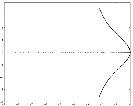
Figure 1: Complex growth factor $\Lambda$ for $0\leq k\leq 2$. Hard spheres.

We have already in the preceding section found that the transverse mode is damped and nonpropagating.

VI Discussion

Let us pull out the acceleration from the viscous pressure tensor $\mathbf{P}_{h}$ using (7 )

$$\mathbf{P}_{h}=(\varpi_{2}-\varpi_{3})\frac{\mu^{2}}{p}\langle(\mathbf{\nabla}\frac{D\mathbf{v}}{Dt})\rangle+\mathbf{\tilde{P}}_{h}.$$

Here

$$\mathbf{\tilde{P}}_{h}=p\mathbf{1}-2\mu\mathbf{S}+\varpi_{1}\frac{\mu^{2}}{p}(\mathbf{\nabla}\cdot\mathbf{v})\,\mathbf{S}$$

$$-(\varpi_{2}-\varpi_{3})\frac{\mu^{2}}{p}\langle(\mathbf{\nabla v})^{2}\rangle$$

$$-2\varpi_{2}\frac{\mu^{2}}{p}\langle\mathbf{S}\cdot(\mathbf{\nabla v})\rangle-\varpi_{3}\frac{\mu^{2}}{\rho^{2}}\langle\mathbf{\nabla\nabla}\rho\rangle$$

$$+\varpi_{3}\frac{\mu^{2}}{\rho T}\langle-\frac{1}{\rho}\mathbf{\nabla}T\mathbf{\nabla}\rho+\frac{T}{\rho^{2}}\mathbf{\nabla}\rho\mathbf{\nabla}\rho-\frac{p}{\rho T}(\mathbf{\nabla v)}^{2}\rangle$$

$$+\varpi_{4}\frac{\mu^{2}}{\rho pT}\langle\mathbf{\nabla}\,p\mathbf{\nabla}\,T\rangle+\varpi_{5}\frac{\mu^{2}}{\rho T^{2}}\langle\mathbf{\nabla}\,T\mathbf{\nabla}\,T\rangle$$

$$+\varpi_{6}\frac{\mu^{2}}{p}\langle\mathbf{S}\cdot\mathbf{S}\rangle.$$

The momentum equation can now be written

$$\rho\frac{D\mathbf{v}}{Dt}-\mathbf{\nabla}\cdot[(\varpi_{3}-\varpi_{2})\frac{\mu^{2}}{p}\langle(\mathbf{\nabla}\frac{D\mathbf{v}}{Dt})\rangle]=-\mathbf{\nabla\cdot\tilde{P}}_{h}.$$

Let us write $\mathbf{a}$ for the acceleration and study the terms containing the acceleration

$$\rho\mathbf{a}-\mathbf{\nabla}\cdot[(\varpi_{3}-\varpi_{2})\frac{\mu^{2}}{p}\langle\mathbf{\nabla a}\rangle]$$

We multiply by $\mathbf{a}$ and integrate over the region of flow

$$\int\{\mathbf{a}\cdot[\rho\mathbf{a}-\mathbf{\nabla}\cdot((\varpi_{3}-\varpi_{2})\frac{\mu^{2}}{p}\langle\mathbf{\nabla a}\rangle)]\}dV$$

$$= \int[\rho a^{2}+(\varpi_{3}-\varpi_{2})\frac{\mu^{2}}{p}\langle\mathbf{\nabla a}\rangle:\langle\mathbf{\nabla a}\rangle]dV$$

$$- \int(\varpi_{3}-\varpi_{2})\frac{\mu^{2}}{p}\mathbf{a}\cdot\langle\mathbf{\nabla a}\rangle\cdot d\mathbf{S}$$

If there are no boundaries and the flow vanishes at infinity, the surface integral vanishes. We conclude that the operator acting on $D\mathbf{v}/Dt$ is then positive and the momentum equation can be solved for the acceleration. The situation when there are boundaries requires a closer examination.

In order to see more clearly the structure of the hybrid Burnett equations, we replace the nonlinear terms in $K\!n^{2}$ by dots. But first we split up in longitudinal and transverse parts according to

$$\frac{1}{2}\triangle+\frac{1}{6}\mathbf{\nabla\nabla}=\frac{2}{3}\mathbf{\nabla\nabla}+\frac{1}{2}(\triangle-\mathbf{\nabla\nabla}).$$

The hybrid Burnett equations can then be written

$$\frac{D\rho}{Dt}+\rho(\mathbf{\nabla\cdot v})=0,$$ (19)

$$\rho\{\mathbf{1}-(\varpi_{3}-\varpi_{2})\frac{\mu^{2}}{p\rho}[\frac{1}{2}(\triangle\mathbf{1-\nabla\nabla})+\frac{2}{3}\mathbf{\nabla\nabla}\}\cdot\frac{D\mathbf{v}}{Dt}$$ (20)

$$=-\mathbf{\nabla}p+2\mathbf{\nabla}\cdot(\mu\mathbf{S})+\varpi_{3}\frac{\mu^{2}}{\rho^{2}}\frac{2}{3}\triangle\mathbf{\nabla}\rho+...,$$

$$\frac{3k_{B}}{2m}\rho\frac{DT}{Dt}=-p(\mathbf{\nabla}\cdot\mathbf{v})+2\mu\mathbf{S}\cdot\mathbf{S}+\mathbf{\nabla}\cdot(\kappa\,\mathbf{\nabla}\,\,T)$$ (21)

$$-(\theta_{4}-\theta_{2})\frac{\mu^{2}}{\rho}\frac{2}{3}\triangle(\mathbf{\nabla}\cdot\mathbf{v})+...$$

Let us also write down the momentum equation of the conventional Burnett equations There is no need to write down the equations of continuity and energy as they are exactly the same as for the hybrid equations.

$$\rho\frac{D\mathbf{v}}{Dt}=-\mathbf{\nabla}p+2\mathbf{\nabla}\cdot(\mu\mathbf{S})-(\varpi_{3}-\varpi_{2})\frac{\mu^{2}}{\rho T}\frac{2}{3}\triangle\mathbf{\nabla}T$$ (22)

$$+\varpi_{2}\frac{\mu^{2}}{\rho^{2}}\frac{2}{3}\triangle\mathbf{\nabla}\rho+...$$

The difference is that the hybrid Burnett equations have a more complicated inertia term but no term $\triangle\mathbf{\nabla}T$ in the momentum equation. The coefficient in front of the term $\triangle\mathbf{\nabla}\rho$ is $\varpi_{3}-\varpi_{2}$ in the conventional Burnett equations but $\varpi_{3}$ in the hybrid Burnett equations.

Let us also note that the equations without the $K\!n^{2}$ nonlinear terms are valid when $K\!n^{2}M\!a^{2}$ can be neglected and the relative temperature and density variations are assumed to be of the order of $M\!a$.

Let us take a closer look at the inertia term in the hybrid Burnett equations, see (17). We consider a Fourier component of the acceleration ${D\mathbf{v}}/{Dt}$ proportional to $\exp(i\mathbf{k}\cdot\mathbf{r})$. Then

$$\rho\{[\mathbf{1}-(\varpi_{3}-\varpi_{2})\frac{\mu^{2}}{p\rho}[\frac{1}{2}(\triangle\mathbf{1-\nabla\nabla})\mathbf{+}\frac{2}{3}\mathbf{\nabla\nabla}]\}\frac{D\mathbf{v}}{Dt}$$

$$= \rho\{[1+\frac{1}{2}(\varpi_{3}-\varpi_{2})\frac{\mu^{2}k^{2}}{p\rho}](\mathbf{1}-\frac{\mathbf{kk}}{k^{2}})$$

$$+[1+\frac{2}{3}(\varpi_{3}-\varpi_{2})\frac{\mu^{2}k^{2}}{p\rho}]\frac{\mathbf{kk}}{k^{2}}\}\frac{D\mathbf{v}}{Dt}.$$

We have effectively a transverse inertia in the first term and a longitudinal inertia in the second term. As $\varpi_{3}-\varpi_{2}>0$, both of them are positive. We noted earlier that the sign of the $D\mathbf{v/}Dt$ term of the hybrid Burnett expression for $\mathbf{P}$ is the opposite of that of the original Burnett equations. As a result the original Burnett equations have a singularity for certain wave numbers where the inertia vanishes.

Let us also consider the low $M\!a$ stationary case. The hybrid Burnett equations are then

$$\mathbf{\nabla\cdot(}\rho\mathbf{v}) = 0,$$

$$\rho(\mathbf{v\cdot\nabla})v=-\mathbf{\nabla}p + 2\mathbf{\nabla\cdot(}\mu\mathbf{S})+\varpi_{3}\frac{\mu^{2}}{\rho^{2}}\frac{2}{3}\triangle\mathbf{\nabla}\rho\mathbf{,}$$

$$\frac{3k_{B}}{2m}\rho(\mathbf{v\cdot\nabla}T) = -p\mathbf{(\nabla\cdot v)+}2\mu\mathbf{S}:\mathbf{S}$$

$$+\mathbf{\nabla}\cdot(\kappa\,\mathbf{\nabla}\,T) - (\theta_{4}-\theta_{2})\frac{\mu^{2}}{\rho}\frac{2}{3}\triangle(\mathbf{\nabla}\cdot\mathbf{v}).$$

The conventional Burnett momentum equation is

$$\rho(\mathbf{v\cdot\nabla)v}=-\mathbf{\nabla}p+2\mathbf{\nabla\cdot(}\mu\mathbf{S})$$ (23)

$$-(\varpi_{3}-\varpi_{2}\mathbf{)}\frac{\mu^{2}}{\rho T}\frac{2}{3}\triangle\mathbf{\nabla}T+\varpi_{2}\frac{\mu^{2}}{\rho^{2}}\frac{2}{3}\triangle\mathbf{\nabla}\rho\mathbf{,}$$

The only difference between the hybrid Burnett equations and the conventional Burnett equations is the change of coefficients

$$\varpi_{2}\rightarrow\varpi_{3},\varpi_{3}\rightarrow\varpi_{3}.$$ (24)

This also means that the third derivative of the temperature is absent in the hybrid Burnett equations.

References

• (1) C. Cercignani, Rarefied Gas Dynamics. From Basic Concepts to Actual Calculations. Cambridge University Press, Cambridge (2000).
• (2) G.A. Bird, Molecular Gas Dynamics and the Direct Simulation of Gas Flows. Clarendon Press, Oxford (1995).
• (3) Y. Sone, Kinetic Theory and Fluid Dynamics. Birkhäuser, Boston (2002).
• (4) S. Chapman and T.G. Cowling, The Mathematical Theory of Non-Uniform Gases. Cambridge University Press, Cambridge, 3rd edition, 1970.
• (5) D. Burnett, Proc. London Math. Soc. 40, 382 (1935).
• (6) A.V. Bobylev, Soviet Physics Doklady 27, 29 (1982).
• (7) R.K. Agarwal, K.-Y. Yun & R. Balakrishnan,Phys. Fluids 13, 3061 (2001).
• (8) F. J. Uribe, R. M. Velasco, and L. S. Garcia-Colin , Phys. Rev. E 62, 5835 (2000).
• (9) S. Jin and M. Slemrod, Journal of Statistical Physics 103, 1009 (2001).
• (10) M. Svärd, Mekanik-KTH Master Thesis 14 (1999).
• (11) M. Strömgren, Nada-KTH Master Thesis E02102 (2002).
• (12) L.H. Söderholm, Nonlinear Acoustics to Second Order in Knudsen Number Without Unphysical Instabilities, Rarefied Gas Dynamics 24 (2005) (to be published).
• (13) S. Reinecke & G.M. Kremer, Continuum Mechanics and Thermodynamics, 8, 121 (1996).