Formation of molecules from a Cs Bose-Einstein condensate

Abstract

Conversion of an expanding Bose-Einstein condensate of Cs atoms to a molecular one with an efficiency of more than 30% was observed recently in experiments by M. Mark et al., Europhys. Lett. 69, 706 (2005). The theory presented here describes the experimental results. Values of resonance strength of 8 mG and rate coefficients for atom-molecule deactivation of $1\times 10^{-11}$ cm${}^{3}/$s and molecule-molecule one of $1.5\times 10^{-9}$ cm${}^{3}/$s are estimated by a fit of the theoretical results to the experimental data. Near the resonance, where the highest conversion efficiency was observed, the results demonstrate strong sensitivity to the magnetic field ripple and inhomogeneity. A conversion efficiency of about 60% is predicted by non-mean-field calculations for the densities and sweep rates lower than the ones used in the experiments.

Introduction

A molecular Bose-Einstein condensate (BEC) has been recently formed in experiments on atomic BEC HKMWCNG03 ; MKHCNG04 ; DVMR03 ; DVMR04 ; XMACMK03 ; MAXCK04 and on quantum-degenerate Fermi gases RTBJ03 . The molecules have been formed by sweeping the Zeeman shift through a Feshbach resonance (see Ref. TTHK99 ) in a backward direction, so that the molecular state crossed the atomic ones downwards. This led to the transfer of population from the lowest atomic state in the case of a BEC, or from an energy band in the case of a Fermi gas, to the molecular state, as had been proposed in Ref. MTJ00 . Assuming all the atomic population is initially in the BEC state, the backward sweep would have been ideally suitable for forming molecules, were it not for two loss mechanisms. The resonant molecule is generally populated in an excited rovibrational and electronic state, and therefore can be deactivated by exoergic inelastic collisions with atoms and other molecules (see Refs. TTHK99 ; YBJW99 ; AV99 ; YBJW00 ). (A stabilization of molecules by means of coherent control SB03 has been considered in Ref. LKMV04 .) In addition, during the backward sweep, some higher-lying non-condensate atomic states can be populated temporarily due to molecular dissociation. These two effects restrict the efficiency of conversion from the atomic BEC to the molecular one.

Formation of molecular BEC from degenerate Fermi gases, realized in experiments RTBJ03 , is more efficient due to Pauli blocking of inelastic collisions P03 . Some peculiarities of this process have been discussed in Ref. PVB04 . In the case of Bose atoms the deactivation losses can be minimized by a reduction of the condensate density (see Ref.  YB03 ). Such a reduction can be realized in experiments by using an expanding BEC, released from a trap by turning it off (see Refs. HKMWCNG03 ; MKHCNG04 ; DVMR03 ; DVMR04 ). A conversion efficiency of more than 30%, comparable to the one obtained for Fermi gases, has been achieved by this way in Cs experiments MKHCNG04 .

The present work provides a theoretical description of molecular formation in an expanding BEC with applications to the Cs experiments MKHCNG04 , including an explanation of the high conversion efficiency. Some of the results obtained below can be satisfactory derived by a mean-field theory. However, in general, a description of certain processes, such as the spontaneous dissociation of the molecular BEC into non-condensate entangled atom pairs discussed in Sec. I below requires the use of a non-mean-field theory. Several theoretical methods are available for this purpose. One such method is based on a numerical solution of stochastic differential equations in the positive-$P$ representation, as used in the present context in Ref. PM01 . Another method is the Hartree-Fock-Bogoliubov formalism (see Refs. HPW01 ; KH02 ), which deals with coupled equations for the atomic and the molecular mean fields, as well as the normal and the anomalous densities describing the second-order correlations of the non-condensate atomic fields. These correlations are also taken into account in the microscopic quantum dynamics approach used in Ref. KB02 . Some of these methods, however, have no room for incorporating the deactivating collisions. The parametric approximation used in Refs. YB03 ; VYA01 ; YB04 ; Y05 incorporates both the non-mean-field effects and the damping due to deactivating collisions.

The present work is organized in the following way. Section I describes the various processes in a hybrid atom-molecule condensate and theoretical methods needed for their analysis. The necessary parameters of the Cs BEC are estimated in Sec. II by a fit of calculation results to the experimental data. The formation of molecules in the switching scheme, one of the two sweeping methods used in the experiment MKHCNG04 and discussed in Sec. II below, is analyzed in Sec. III. Optimal conditions for the molecular formation are determined in Sec. IV.

I Theoretical methods

The effect of Feshbach resonance appears in a BEC of Cs atoms when the collision energy of a pair of atoms in an open channel is close to the energy of a bound state Cs${}_{2}\left(m\right)$ in a closed channel (see Ref. TTHK99 ). The temporary formation and dissociation of the resonant (Feshbach) molecular state Cs${}_{2}\left(m\right)$ can be described as a reversible reaction

$$\text{Cs + Cs }\rightleftarrows\text{ Cs}_{2}\left(m\right).$$ (1)

The Cs${}_{2}\left(m\right)$ is an excited rovibrational state with orbital angular momentum $l=4$, belonging to an excited state of the fine and hyperfine structures. This state can be deactivated by an exoergic collision with a third atom of the condensate TTHK99 ; YBJW99 ; AV99 ; YBJW00 ,

$$\mathrm{Cs}_{2}(m)+\text{Cs}\rightarrow\text{Cs}_{2}(d)+\text{Cs , }$$ (2)

bringing the molecule down to a lower state Cs${}_{2}\left(d\right)$, and releasing kinetic energy to the relative motion of the reaction products. Although the collision occurs with a vanishingly small kinetic energy, rates of such inelastic processes remain finite at near-zero energies MAXCK04 ; Forrey99 . A variant of this process, involving deactivation by a collision with another molecule (rather than an atom), of the type

$$\mathrm{Cs}_{2}(m)+\mathrm{Cs}_{2}(m)\rightarrow\text{Cs}_{2}\left(d\right)+\text{Cs}_{2}\left(u\right),$$ (3)

would require a significant molecular density to be effective. The two molecular states Cs${}_{2}\left(d\right)$ and Cs${}_{2}\left(u\right)$ can be distinct.

A complete analysis of the processes in a hybrid atom-molecule BEC must take into account both the relaxation processes due to deactivating collisions (2) and (3), and the quantum fluctuations due to dissociation of the resonant molecules to non-condensate atoms (1). A starting point of such an analysis can be the quantum equation of motion for the atomic field annihilation operator $\hat{\Psi}_{a}\left({\bf p},t\right)$ in the momentum representation. An adiabatic elimination of the “dump” states Cs${}_{2}\left(d\right)$ and Cs${}_{2}\left(u\right)$ (see Refs. YB03 ; Y05 ) reduces this equation to the Heisenberg-Langevin stochastic equation

$$i\hbar\dot{\hat{\Psi}}_{a}\left({\bf p},t\right)=\left[{p{}^{2}\over 2m}+\epsilon_{a}\left(t\right)-i{k{}_{a}\over 2}|\varphi_{m}\left(t\right)|^{2}\right]\hat{\Psi}_{a}\left({\bf p},t\right)$$

$$+2g^{*}\varphi_{m}\left(t\right)\hat{\Psi}^{{\dagger}}_{a}\left(-{\bf p},t\right)+i\hat{F}\left({\bf p},t\right).$$ (4)

Here $m$ is the atomic mass, $\epsilon_{a}\left(t\right)=-{1\over 2}\mu\left(B\left(t\right)-B_{0}\right)$ is the time-dependent Zeeman shift of the atom in an external magnetic field $B\left(t\right)$ relative to half the energy of the molecular state (which is fixed as the zero-energy point), $\mu$ is the difference between the magnetic momenta of an atomic pair and a molecule, and $B_{0}$ is the resonance value of $B$. The atom-molecule hyperfine coupling $g$ is related to the phenomenological resonance strength $\Delta$ through $|g|^{2}=2\pi\hbar^{2}|a_{a}|\mu\Delta/m$ (see Ref. YBJW00 ), where $a_{a}$ is the background elastic scattering length for atom-atom collisions. The deactivation (2) by atom-molecule collisions is represented in Eq. (4) by the imaginary term, proportional to the deactivation rate $k_{a}$, as well as by the quantum noise source $\hat{F}\left({\bf p},t\right)$, related by a fluctuation-dissipation theorem. The quantum noise is required in order to maintain the correct commutation relations of the atomic field operators.

In the parametric approximation YB03 ; Y05 , the quantum fluctuations of the molecular field are neglected, and the molecules are described by a mean field $\varphi_{m}\left(t\right)$. The atomic field operator is expressed in this method as

$$\hat{\Psi}_{a}\left({\bf p},t\right)=C\left(t\right)\left[\hat{A}\left({\bf p},t\right)\psi_{c}\left(p,t\right)+\hat{A}^{{\dagger}}\left(-{\bf p},t\right)\psi_{s}\left(p,t\right)\right],$$ (5)

where the damping factor $C\left(t\right)$ takes into account the imaginary term in Eq. (4),

$$C\left(t\right)=\exp\left(-\int\limits^{t}_{t{}_{0}}dt_{1}{k{}_{a}\over 2}|\varphi_{m}\left(t_{1}\right)|^{2}\right),$$ (6)

and the $c$-number functions $\psi_{c,s}\left(p,t\right)$ satisfy the ordinary differential equations (with $p$ as a parameter)

$$i\hbar\dot{\psi}_{c,s}\left(p,t\right)=\left[{p{}^{2}\over 2m}+\epsilon_{a}\left(t\right)\right]\psi_{c,s}\left(p,t\right)+2g^{*}\varphi_{m}\left(t\right)\psi^{*}_{s,c}\left(p,t\right).$$ (7)

The initial conditions $\psi_{c}\left(p,t_{0}\right)=1$, $\psi_{s}\left(p,t_{0}\right)=0$ are introduced at $t=t_{0}$, assuming the atomic field is then a coherent state of zero kinetic energy. The operators $\hat{A}\left({\bf p},t\right)$ can be expressed in terms of the functions $\psi_{c,s}\left(p,t\right)$ and the quantum noise $\hat{F}\left({\bf p},t\right)$. As a result of ensuing analysis (see Refs. YB03 ; Y05 ), the atomic density comprises the sum

$$n_{a}\left(t\right)=n_{0}\left(t\right)+n_{s}\left(t\right)$$ (8)

of the densities of condensate atoms

$$n_{0}\left(t\right)=|\varphi_{0}\left(t\right)|^{2},$$ (9)

and of non-condensate (entangled) atoms

$$n_{s}\left(t\right)=\left(2\pi\hbar\right)^{-3}\int d^{3}pn_{s}\left(p,t\right).$$ (10)

Here

$$\varphi_{0}\left(t\right)=C\left(t\right)\left[\psi_{c}\left(0,t\right)\varphi_{0}\left(t_{0}\right)+\psi_{s}\left(0,t\right)\varphi^{*}_{0}\left(t_{0}\right)\right]$$ (11)

is the atomic condensate mean field. The momentum spectrum of the non-condensate atoms

$$n_{s}\left(p,t\right)=|\psi_{s}\left(p,t\right)|^{2}\left[1+\eta_{s}\left(p,t\right)\right]+|\psi_{c}\left(p,t\right)|^{2}\eta_{s}\left(p,t\right)$$

$$-2\text{Re}\left[\psi^{*}_{s}\left(p,t\right)\psi_{c}\left(p,t\right)\eta_{c}\left(p,t\right)\right],$$ (12)

as well as their anomalous density [encountered in Eq. (15) below]

$$m_{s}\left(p,t\right)=\psi_{s}\left(p,t\right)\psi_{c}\left(p,t\right)\left[1+2\eta_{s}\left(p,t\right)\right]$$

$$-\psi^{2}_{c}\left(p,t\right)\eta_{c}\left(p,t\right)-\psi^{2}_{s}\left(p,t\right)\eta^{*}_{c}\left(p,t\right),$$ (13)

are expressed in terms of the auxiliary functions

$$\eta_{s}\left(p,t\right)=k_{a}C^{2}\left(t\right)\int\limits^{t}_{t{}_{0}}{dt^{\prime}\over C^{2}\left(t^{\prime}\right)}|\varphi_{m}\left(t^{\prime}\right)\psi_{s}\left(p,t^{\prime}\right)|^{2}$$

(14)

$$\eta_{c}\left(p,t\right)=k_{a}C^{2}\left(t\right)\int\limits^{t}_{t{}_{0}}{dt^{\prime}\over C^{2}\left(t^{\prime}\right)}|\varphi_{m}\left(t^{\prime}\right)|^{2}\psi_{s}\left(p,t^{\prime}\right)\psi^{*}_{c}\left(p,t^{\prime}\right),$$

which describe the contribution of quantum noise.

The equation of motion for the molecular mean field has the form (see Refs. YB03 ; Y05 )

$$i\hbar\dot{\varphi}_{m}\left(t\right)=g\varphi^{2}_{0}\left(t\right)-i\left({k{}_{a}\over 2}n_{a}\left(t\right)+k_{m}|\varphi_{m}\left(t\right)|^{2}\right)\varphi_{m}\left(t\right)$$

$$+{1\over 2\pi^{2}\hbar{}^{3}}\int\limits^{\infty}_{0}dp\left[p^{2}gm_{s}\left(p,t\right)+2\hbar m|g|^{2}\varphi_{m}\left(t\right)\right],$$ (15)

where $k_{m}$ is the rate coefficient of the molecule-molecule deactivating collisions (3). The second term under the integral over $p$ appears as a result of a renormalization procedure (see Refs. HPW01 ; Y05 ), necessary in order to regularize the integral. A numerical solution of Eqs. (7) on a grid of values of $p$, combined with Eq. (15), is consistently sufficient for elucidating the dynamics of the system.

The parametric approximation considered above is particularly suitable for the analysis of homogeneous systems. It can be applied also to inhomogeneous systems using a local density approximation, but its application to a strongly inhomogeneous expanding BEC meets serious difficulties. Fortunately, under proper conditions this case can be treated sufficiently well by a mean field approach (see Ref. YB04 ), neglecting the atomic field quantum fluctuations. The applicability of this simpler approach can be verified by a comparison of results of the parametric and mean-field calculations for the corresponding homogeneous system.

The expansion of a pure atomic BEC has been considered in Ref. expan by the introduction of scaled normal coordinates

$$\rho_{j}=r_{j}/b_{j}\left(t\right),1\leq j\leq 3,$$ (16)

where the scales $b_{j}$ obey the equations

$$\ddot{b}_{j}\left(t\right)=\omega^{2}_{j}/\left[b_{1}\left(t\right)b_{2}\left(t\right)b_{3}\left(t\right)b_{j}\left(t\right)\right],$$ (17)

in which the $\omega_{j}$ are the angular frequencies of the harmonic trap containing the condensate before expansion. The initial conditions $b_{j}\left(t_{\exp}\right)=1$, $\dot{b}_{j}\left(t_{\exp}\right)=0$ are stated at the start of the expansion $t_{\exp}$. Solutions of Eq. (17) (see Ref. expan ) demonstrate that the expansion is ballistic after an acceleration period of $\sim\min\left(\omega^{-1}_{j}\right)$. As shown in Ref. YB04 , the molecules inherit the velocity of the atoms they are formed from. The atomic and molecular mean fields can be represented in terms of rescaled fields $\Phi_{0}\left(\bm{\rho},t\right)$ and $\Phi_{m}\left(\bm{\rho},t\right)$, respectively, as

$$\varphi_{0}\left({\bf r},t\right)=A\left(t\right)\Phi_{0}\left(\bm{\rho},t\right)e^{i}{}^{S}$$

(18)

$$\varphi_{m}\left({\bf r},t\right)=A\left(t\right)\Phi_{m}\left(\bm{\rho},t\right)e^{2i}{}^{S},$$

where the scaling factor $A\left(t\right)=\left(b_{1}\left(t\right)b_{2}\left(t\right)b_{3}\left(t\right)\right)^{-1/2}$ describes the density reduction, and the phase factor with

$$S\left(t\right)={m\over\hbar}\sum\limits^{3}_{j=1}r^{2}_{j}{\dot{b}_{j}\left(t\right)\over 2b_{j}\left(t\right)}-{\epsilon{}_{0}\over\hbar}\int\limits^{t}_{t{}_{\exp}}dt^{\prime}A^{2}\left(t^{\prime}\right)$$ (19)

contains most of the contribution of the kinetic energy. Here $\epsilon_{0}=4\pi\hbar^{2}a_{a}n_{0}/m$ is a chemical potential of the atomic BEC and $n_{0}$ is its peak density while the trap is on. As a result ( see Ref. YB04 ), the rescaled mean fields obey the set of ordinary differential equations

$$i\hbar\dot{\Phi}_{0}\left(\bm{\rho},t\right)=\left[\epsilon_{a}\left(t\right)-{i\over 2}A^{2}\left(t\right)k_{a}|\Phi_{m}\left(\bm{\rho},t\right)|^{2}\right]\Phi_{0}\left(\bm{\rho},t\right)$$

$$+2A\left(t\right)g^{*}\Phi^{*}_{0}\left(\bm{\rho},t\right)\Phi_{m}\left(\bm{\rho},t\right)$$

(20)

$$i\hbar\dot{\Phi}_{m}\left(\bm{\rho},t\right)=-iA^{2}\left(t\right)\biggl{[}{1\over 2}k_{a}|\Phi_{0}\left(\bm{\rho},t\right)|^{2}$$

$$+k_{m}|\Phi_{m}\left(\bm{\rho},t\right)|^{2}\biggr{]}\Phi_{m}\left(\bm{\rho},t\right)+A\left(t\right)g\Phi^{2}_{0}\left(\bm{\rho},t\right).$$

The coordinate dependence arises from the use of inhomogeneous Thomas-Fermi initial conditions for $\Phi_{0}\left(\bm{\rho},t_{\exp}\right)$, while $\Phi_{m}\left(\bm{\rho},t_{\exp}\right)=0$.

II Parameter estimates

Molecules have been formed in the experiments MKHCNG04 by using a very weak Feshbach resonance in Cs situated near 20 G. The resonance strength and the rate coefficients of atom-molecule and molecule-molecule deactivation are unknown and are estimated here by a fit of the calculation results to the experimental data.

The magnetic field has been varied in these experiments in two manners. In the ramping scheme the magnetic field has been swept through resonance with a fixed ramp speed. In the switching scheme the magnetic field has been tuned to a value $B_{\text{test}}$ in the vicinity of the resonance and then held for a fixed time $t_{\text{hold}}$, starting from the value $B_{\text{start}}=B_{0}\pm 0.5$ G for $B_{\text{test}}\gtrless B_{0}$, respectively, so that the resonance should not be crossed. Due to finite response time the magnetic field variation is represented by an exponential function,

$$B\left(t\right)=B_{\text{test}}+\left(B_{\text{start}}-B_{\text{test}}\right)\exp\left[\left(t-t_{\exp}\right)/1.54\text{ ms}\right].$$ (21)

The switching scheme has been applied both to the trapped and the expanding BEC. In the last case, the magnetic field variation has been started from $B_{\text{start}}$ simultaneously with the expansion at $t=t_{\exp}$.

Figure 1: Switching-scheme atom loss fraction calculated for the trapped BEC with $\Delta=8$ mG, $k_{m}=1.5\times 10^{-9}$ cm${}^{3}/$s, $k_{a}=1\times 10^{-11}$ cm${}^{3}/$s (solid line) and $k_{a}=2\times 10^{-11}$ cm${}^{3}/$s (dot-dashed line). The results for $k_{m}=1\times 10^{-10}$ cm${}^{3}/$s are calculated with $\Delta=8$ mG, $k_{a}=1\times 10^{-11}$ cm${}^{3}/$s (dashed line) and $\Delta=2$ mG, $k_{a}=4\times 10^{-11}$ cm${}^{3}/$s (pluses). The open and solid circles represent the experimental data of Ref. MKHCNG04 measured below and above the resonance, respectively.

Consider first the switching scheme for a trapped BEC, resulting in a condensate loss with a negligible molecular formation. This experiment is similar to the slow-sweep Na experiments MIT_Na_loss and the ⁸⁷Rb experiments M02 , in which the field was stopped short of resonance, too. In those cases the condensate loss is determined by simple analytical expressions involving the product of the resonance strength $\Delta$ and the atom-molecule deactivation rate coefficient $k_{a}$ (see Refs. YBJW99 ; YBJW00 ; YB03b ). In the present case, these analytical expressions are inapplicable owing to the non-linear magnetic field variation. However, numerical calculations still demonstrate a dependence on the product $k_{a}\Delta$ provided moderate molecule-molecule deactivation rates are assumed. (This is demonstrated by the dashed line and pluses in Fig. 1). The comparison with the experimental data leads to an estimated value of $k_{a}\Delta\approx 8\times 10^{-11}$ mG cm${}^{3}/$s. Much higher values of $k_{m}$ do not lead to such a good fit. Although the condensate loss becomes dependent on a variation of $k_{a}$ and $\Delta$, keeping the product $k_{a}\Delta$ fixed, this variation does not improve the fit.

Figure 2: Ramping-scheme atom loss fraction (l) and conversion efficiency (c) calculated for the expanding BEC with $k_{m}=1.5\times 10^{-9}$ cm${}^{3}/$s, $k_{a}\Delta=8\times 10^{-11}$ mG cm${}^{3}/$s, and $\Delta=8$ mG (solid lines), $\Delta=7$ mG (dashed lines), or $\Delta=9$ mG (dot-dashed lines). The results for $\Delta=8$ mG and $k_{a}=1\times 10^{-11}$ cm${}^{3}/$s are represented by pluses ($k_{m}=2\times 10^{-9}$ cm${}^{3}/$s) and crosses ($k_{m}=1\times 10^{-9}$ cm${}^{3}/$s). The open and solid circles represent the experimental data of Ref. MKHCNG04 for loss and conversion, respectively.

Consider now the ramping scheme. It has been applied in experiments MKHCNG04 to the expanding BEC, measuring both the numbers of remained atoms and formed molecules. In the fast-decay approximation (see Refs. YBJW99 ; YBJW00 ), the atomic condensate loss due to the resonance crossing is determined by the resonance strength $\Delta$ only and is independent of the deactivation rates. Although the analytical expressions of Refs. YBJW99 ; YBJW00 are inapplicable to the case of an expanding BEC, the results of numerical calculations demonstrate a low sensitivity of the BEC loss to the deactivation rates. A comparison with the experimental data leads to the estimated value of $\Delta\approx 8$ mG (see the upper graphs in Fig. 2). Together with the above estimate for $k_{a}\Delta$ this leads to $k_{a}\approx 1\times 10^{-11}$ cm${}^{3}/$s. The experimental data points presented in Fig. 2 were obtained with a magnetic field ramp that has been started at $t_{\exp}$, using a magnetic field value such that the resonance is crossed in 10 ms and the populations are measured 20 ms after $t_{\exp}$ ChinPC .

The remaining unknown parameter, the molecule-molecule deactivation rate coefficient $k_{m}$, can be estimated by a comparison of the calculation results with the experimental data for the number of atoms converted to molecules (see lower graphs in Fig. 2). This leads to the estimated value of $k_{m}\approx 1.5\times 10^{-9}$ cm${}^{3}/$s. The graphs in Fig. 2 are practically insensitive to $k_{a}$ because of its much lower value. A look back at Fig. 1 for the switching scheme shows that, at most, $k_{a}$ is bounded by $k_{a}<2\times 10^{-11}$ cm${}^{3}/$s, when the far-off-resonance results are regarded. In this range, the results are not much sensitive to the value of $k_{m}$. However, nearer resonance, the higher value of $k_{m}$ would lead to an overestimate of the loss, independently of $k_{a}$ and $\Delta$.

Let us compare these values with what is known regarding other atoms. The estimated value of the rate coefficient of atom-molecule deactivation $k_{a}\approx 10^{-11}$ cm${}^{3}/$s is several times lower than the corresponding values of $5.5\times 10^{-11}$ cm${}^{3}/$s for Na measured in Ref. MAXCK04 and $7\times 10^{-11}$ cm${}^{3}/$s for ⁸⁷Rb estimated in Ref. YB03b . A molecule-molecule deactivation rate coefficient $k_{m}\approx 1.5\times 10^{-9}$ cm${}^{3}/$s exceeds the corresponding value for Na $2.5\times 10^{-11}$ cm${}^{3}/$s measured in Ref. MAXCK04 by two orders of magnitude. These differences may be related to the large orbital angular momentum ($l=4$) of the resonant molecular state in the present Cs case, while for Na and ⁸⁷Rb $l=0$. But there may be another reason.

All the estimates made here concerning the data for molecular conversion are based on the suggestion that the resonant beam, blasting out the atoms in the experiments MKHCNG04 , does not affect the molecules. (This procedure was used to separate the atoms from molecules.) If some part of the molecular population is removed by the blasting pulse, the experimental results can be explained using lower values of $k_{m}$.

Figure 3: Time dependence of the atomic (a) and molecular (m) condensate populations (scaled to the initial atomic one) calculated in a ramping scheme for a homogeneous BEC with the initial atomic density $6.4\times 10^{11}$ cm^-3, ramp speed 3 G/s (in the backward sweep), $\Delta=8$ mG, $k_{a}=1\times 10^{-11}$ cm${}^{3}/$s, and $k_{m}=1\times 10^{-9}$ cm${}^{3}/$s with the parametric (solid lines) and mean-field (crosses) approximations. The dashed lines represent the mean field results for the expanding BEC with the initial atomic density $7.6\times 10^{13}$ cm^-3. The non-condensate atom population calculated with the parametric approximation is plotted by the dot-dashed line.

All the calculations above were performed with the mean field approximation. Figure 3 compares results of the parametric and mean-field calculations for the initial atomic density of $6.4\times 10^{11}$ cm^-3, corresponding to the mean density at the resonance crossing for the slowest ramp speed of 3 G/s used in the experiments MKHCNG04 . This figure demonstrates that the temporary non-condensate atom population persists only about 1 ms and after this short time the results of parametric and mean-field calculations for the homogeneous case coincide within a good accuracy. The expansion reduces the deactivation losses compared to the ones for the homogeneous case.

III Molecular formation in the switching scheme

The highest conversion efficiency, reaching beyond 30%, has been observed in the experiments MKHCNG04 for the switching scheme in an expanding BEC. The characteristic time of atom-molecule relaxation $t_{am}$ is determined by the coupling terms in Eq. (20) as

$$t^{-1}_{am}\sim|Ag\Phi_{0}|=\left({2\pi|a_{a}|\mu\Delta\over m}n_{0}\right)^{1/2},$$ (22)

where $n_{0}\left(t\right)=|\varphi_{0}\left(t\right)|^{2}$ is non-rescaled atomic condensate density. Even for $n_{0}=10^{12}$ cm^-3, corresponding to the resonance approach time in the experiments MKHCNG04 , $t_{am}\sim 1$ ms is less than the characteristic time of the magnetic field variation (1.54 ms). Therefore the evolution of the atom-molecule condensate is adiabatic. Neglecting the deactivation, it can be described by a quasi-stationary solution of the coupled Gross-Pitaevskii equations (see Ref. TTHK99 )

$$n_{0}={n\over 36}\left(\epsilon\sqrt{\epsilon^{2}+24}-\epsilon^{2}+24\right)$$

(23)

$$n_{m}={n\over 144}\left(2\epsilon^{2}-2\epsilon\sqrt{\epsilon^{2}+24}+24\right),$$

corresponding to the pure atomic BEC ($n_{m}=0$) above the resonance at $\epsilon\rightarrow\infty$. Here $n_{m}=|\varphi_{m}|^{2}$ is the non-rescaled molecular density, $n=n_{0}+2n_{m}$ is the total density of atoms, and

$$\epsilon={2\epsilon{}_{a}\over|g|\sqrt{n}}={B_{0}-B{}_{\text{test}}\over\delta B},\qquad\delta B=\left({2\pi\hbar^{2}|a_{a}|\Delta\over m\mu}n_{0}\right)^{1/2}$$ (24)

is a dimensionless detuning (generally time-dependent). The later fast sweep of the magnetic field going under the resonance, used in the switching scheme, conserves the atomic and molecular densities (23) acquired at $B=B_{\text{test}}$.

The conversion efficiency reaches its maximum

$$2{n{}_{m}\over n}={1\over 3}$$ (25)

when the magnetic field levels off at $\epsilon=0$. In the case of large detunings $|B_{\text{test}}-B_{0}|\gg\delta B$ the molecular density decreases as $n_{m}\sim n\delta B^{2}/\left(B_{\text{test}}-B_{0}\right)^{2}$. Therefore the substantial molecular population and condensate losses induced by the deactivating collisions can take place only while $|B_{\text{test}}-B_{0}|<\delta B\approx 0.2$ mG for $n=10^{12}$ cm^-3.

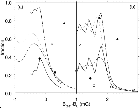
Figure 4: (a) Atom loss fraction (dashed line) and conversion efficiency (solid line) calculated as functions of the resonance detuning for the switching scheme in the expanding BEC with $k_{m}=1.5\times 10^{-9}$ cm${}^{3}/$s, $k_{a}=1\times 10^{-11}$ cm${}^{3}/$s, and $\Delta=8$ mG. The open and solid circles represent the experimental data of Ref. MKHCNG04 for loss and conversion, respectively. The results of calculations for a rippled magnetic field with the phase $\chi=1.25\pi$ are plotted by dot-dashed (conversion) and dashed (loss) lines. (b) The loss (dashed line) and conversion (solid line) for $\chi=1.85\pi$. The results for inhomogeneous magnetic field with gradient 1 G/cm are plotted by dot-dashed (conversion) and dashed (loss) lines. In both parts the triangles and circles represent the experimental data of Ref. MKHCNG04 for loss and conversion, respectively.

This conclusion is confirmed by the results of the numerical calculations (see Fig. 4). These results, however, predict a maximal conversion efficiency of 36% for $B_{\text{test}}=B_{0}-0.15$ mG, when the resonance is crossed. The smooth time dependence of the atomic and molecular populations (see Fig. 5) is in agreement with the adiabatic evolution mentioned above. On decreasing further $B_{\text{test}}$ the conversion efficiency decreases, demonstrating Rabbi oscillations due to non-adiabatic effects. The results in Fig. 4 correspond to a resonance approach from above ($B_{\text{start}}=B_{0}+0.5$ G). In the mean field approximation used here, neglecting molecular dissociation with formation of non-condensate atoms, the same results are reached by approaching the resonance from below.

Figure 5: Time dependence of the atom loss fraction (dashed line) and conversion efficiency (solid line) calculated for the switching scheme in the expanding BEC with $\Delta=8$ mG, $k_{m}=1.5\times 10^{-9}$ cm${}^{3}/$s, $k_{a}=1\times 10^{-11}$ cm${}^{3}/$s, and $B_{\text{test}}=-0.15$ mG. The open and solid circles represent the experimental data of Ref. MKHCNG04 for loss and conversion, respectively. The results of calculations for a rippled magnetic field with the phase $\chi=1.25\pi$ and $B_{\text{test}}=-0.4$ mG are plotted by dot-dashed (conversion) and dashed (loss) lines.

Although the theory describes the peak conversion efficiency and condensate losses observed in the experiments MKHCNG04 , the actual experimental width of the resonance in conversion and in loss, of 2 mG, is about an order of magnitude more than the theoretical one. This disagreement can be related to magnetic field variation mentioned in Ref. MKHCNG04 .

An ambient magnetic field ripple with a frequency of 50 Hz and an amplitude of 4 mG leads to a quite perceptible effect. Although the experiment has been synchronized with the ripple, the results of calculations demonstrate a strong dependence on the ripple phase. In these calculations the magnetic field time dependence has the form

$$B\left(t\right)=B_{\text{test}}+\left(B_{\text{start}}-B_{\text{test}}\right)\exp\left[\left(t-t_{\exp}\right)/1.54\text{ ms}\right]$$

$$+2\text{ mG }\sin\left[2\pi\times 50\text{ Hz}(t-t_{\exp})+\chi\right].$$ (26)

The variation of the phase $\chi$ leads to a shift of the peak and changes the shape of the magnetic field dependence of the loss and molecule formation (see Fig. 4).

Figure 6: Time dependence of the rippled magnetic field with the phases $\chi=1.25\pi$, $\chi=1.85\pi$ and without ripples for $B_{\text{start}}=0.5$ G (solid lines) and $B_{\text{start}}=-0.5$ G (dashed lines). An arbitrary value of $B_{0}$ is shown here for reference by the dotted line.

The ripple may lead to the formation of molecules due to the resonance crossing in a backward direction (see Fig. 6). The crossing can be non-adiabatic, leading to an oscillating time dependence of the atomic and molecular populations (see Figs. 5 and 7). The oscillations are sensitive to the ripple phase $\chi$ as well. For some values of $\chi$, e. g. $\chi=1.85$, the resonance can be crossed a second time, but in the forward direction, even though the first crossing occurred by approaching from above ($B_{\text{start}}>B_{0}$), given the arbitrary value of $B_{0}$ shown in Fig. 6. In this case, a rather long hold-on-time between the crossing and measurement leads to sharp Rabbi oscillations. These oscillations, however, can be averaged by a magnetic field inhomogeneity with a rather small gradient of 1 mG/cm (see Figs. 4 and 7). Effects of both oscillations and inhomogeneity can broaden the resonance to about 1 mG, which is still less than the experimentally observed value of 2 mG. The additional broadening can be related to the uncontrolled magnetic field variations of about 1 mG mentioned in Ref. MKHCNG04 , the behavior of which is unclear.

Figure 7: Time dependence of the atom loss fraction (dashed line) and conversion efficiency (solid line) calculated for a rippled magnetic field with the phase $\chi=1.85\pi$, and with $B_{\text{test}}=1.7$ mG, $k_{m}=1.5\times 10^{-9}$ cm${}^{3}/$s, $k_{a}=1\times 10^{-11}$ cm${}^{3}/$s, and $\Delta=8$ mG. The results for an inhomogeneous magnetic field with gradient 1 G/cm are plotted by dot-dashed (conversion) and dashed (loss) lines.

The magnetic-field time dependence (26) can lead to different results in approaching the resonance from below, with $B_{\text{start}}<B_{0}$, due to an additional resonance crossing occurring earlier. This forward crossing can lead to additional condensate losses due to molecular dissociation into pairs of non-condensate atoms. This dissociation can, however, be reversible, as the non-condensate atoms can associate to molecules during the following backward crossing. A correct analysis of these effects requires the application of non-mean-field calculations to the expanding BEC, in order to obtain reliable conversion estimates.

Figure 8: (a) Conversion efficiency (solid line) at the optimal ramp speed (dashed line). (b) The lifetime of the molecular condensate (solid line) and the time after the resonance crossing when the peak molecular density is reached (dashed line), using the appropriate optimal ramp speed.

Figure 9: Conversion efficiency (solid line) and the lifetime of the molecular condensate (dashed line) as a function of the ramp speed for the initial atomic density $5\times 10^{10}$ cm^-3.

Figure 10: Time dependence of the atomic (dashed line) and molecular (solid line) condensate populations (scaled to the initial atomic one) calculated for a homogeneous BEC with the initial atomic density $5\times 10^{10}$ cm^-3 and ramp speed 35 mG/s (in the backward sweep). The non-condensate atom population is plotted by the dot-dashed line. The resonance is crossed at $t=0$.

IV Optimal conditions

Having a model consistent with the experimental data, we can proceed to determine optimal conditions for the molecular formation. In the switching scheme, when the magnetic field adiabatically approaches the resonance and further suddenly crosses it, the conversion efficiency is restricted by the value of ${1\over 3}$ (see Eq. (25). An adiabatic crossing, as in the ramping scheme, allows for higher results since the adiabatic state (23) corresponds to a total conversion ($n_{m}=n/2$) in the limit of $\epsilon\rightarrow\infty$ below the resonance. As in the cases of Na YB03 and ⁸⁷Rb YB04 ; Y05 , the optimal ramp speed is determined by a balance of the atomic association, decreasing at faster sweeps, and deactivation losses, increasing at slower sweeps. Thus, a sudden sweep would lead to no association, while an infinitely slow adiabatic sweep would lead to total association, accompanied by a total deactivation loss during the infinite time. The optimal density is determined by a concurrence of deactivation losses, increasing at high densities, and dissociation into non-condensate atoms, increasing at low densities. An analysis taking account of the latter loss process requires a non-mean-field theory, such as the parametric approximation. It was mentioned in Sec. I above that this approximation has its limitations in dealing with expanding gases. However, the effect of increasing density due to expansion is less important at the rather low optimal density, stated below, compared to the conditions pertaining to Fig. 3. For these reasons the optimal conditions are determined by using the parametric approximation for a homogeneous non-expanding BEC.

The results presented in Fig. 8 show an optimal initial atomic density of $5\times 10^{10}$ cm^-3. This value corresponds to the mean density of a Thomas-Fermi distribution with a peak density of $1.25\times 10^{11}$ cm^-3. Under the conditions of the experiments MKHCNG04 , this density can be reached after 35 ms of expansion. The optimal ramp speed of 35 mG /s is much slower than the one used in the experiments. The high conversion efficiency does not change much when the ramp speed is varied by about a order of magnitude (see Fig. 9). Figure 10 shows that the molecular density reaches its maximum in about 8 ms after the resonance crossing, or about 0.25 mG below the resonance, and the ramp should be started about 2 mG above it. This figure demonstrates also a substantial population of non-condensate atoms, justifying the necessity to use non-mean-field calculations.

Conclusions

The loss of Cs atomic BEC and formation of a molecular BEC observed in the experiments MKHCNG04 can be described by a mean-field theory of an expanding atom-molecule BEC. A fit of the calculation results to the experimental data leads to estimated values of the resonance strength and rate coefficients for atom-molecule and molecule-molecule deactivating collisions. At small detunings the results are sensitive to magnetic field ripple and inhomogeneity. A determination of optimal conditions for the molecular formation requires a non-mean-field parametric approximation, taking into account the dissociation of molecules into non-condensate atomic pairs. A conversion efficiency of 60% is predicted for lower densities and slower sweeps than the ones used in the experiments.

- (1) J. Herbig, T. Kraemer, M. Mark, T. Weber, C. Chin, H.-C. Nagerl, and R. Grimm, Science 301, 1510 (2003).
- (2) M. Mark, T. Kraemer, J. Herbig, C. Chin, H.-C. Nagerl, and R. Grimm, Europhys. Lett. 69, 706 (2005).
- (3) S. Dürr, T. Volz, A. Marte, and G. Rempe, Phys. Rev. Lett. 92, 020406 (2004).
- (4) S. Dürr, T. Volz, and G. Rempe, Phys. Rev. A 70, 031601(R) (2004).
- (5) K. Xu, T. Mukaiyama, J. R. Abo-Shaeer, J. K. Chin, D. E. Miller, and W. Ketterle, Phys. Rev. Lett. 91, 210402 (2003).
- (6) T. Mukaiyama, J. R. Abo-Shaeer, K. Xu, J. K. Chin, and W. Ketterle, Phys. Rev. Lett. 92, 180402 (2004).
- (7) C. A. Regal, C. Ticknor, J. L. Bohn, and D. S. Jin, Nature 424, 47 (2003); M. Greiner, C.A. Regal, and D. S. Jin, Nature 426, 537 (2003); K. E. Strecker, G. B. Partridge, and R. G. Hulet, Phys. Rev. Lett. 91, 080406 (2003); J. Cubizolles, T. Bourdel, S. J. J. M. F. Kokkelmans, G. V. Shlyapnikov, and C. Salomon, Phys. Rev. Lett. 91, 240401 (2003); T. Bourdel, L. Khaykovich, J. Cubizolles, J. Zhang, F. Chevy, M. Teichmann, L. Tarruell, S. J. J. M. F. Kokkelmans, and C. Salomon,, Phys. Rev. Lett. 93, 050401 (2004); S. Jochim, M. Bartenstein, A. Altmeyer, G. Hendl, C. Chin, J. H. Denschlag, and R. Grimm, Phys. Rev. Lett. 91,240402 (2003); S. Jochim, M. Bartenstein, A. Altmeyer, G. Hendl, S. Riedl, C. Chin, J. H. Denschlag, and R. Grimm, Science 302, 2101 (2003); M.W. Zwierlein, C. A. Stan, C. H. Schunck, S.M. F. Raupach, S. Gupta, Z. Hadzibabic, and W. Ketterle, Phys. Rev. Lett. 91, 250401 (2003); J. Kinast, S. L. Hemmer, M. E. Gehm, A. Turlapov, J. E. Thomas, Phys. Rev. Lett. 92, 150402 (2004).
- (8) E. Timmermans, P. Tommasini, M. Hussein, and A. Kerman, Phys. Rep. 315, 199 (1999).
- (9) F. H. Mies, E. Tiesinga, and P. S. Julienne, Phys. Rev. A 61, 022721 (2000).
- (10) V. A. Yurovsky, A. Ben-Reuven, P. S. Julienne and C. J. Williams, Phys. Rev. A 60, R765 (1999);
- (11) F. A. van Abeelen, and B. J. Verhaar, Phys. Rev. Lett. 83, 1550 (1999).
- (12) V. A. Yurovsky, A. Ben-Reuven, P. S. Julienne and C. J. Williams, Phys. Rev. A 62, 043605 (2000).
- (13) M. Shapiro and P. Brumer Principles of the Quantum Control of Molecular Processes (John Wiley and Sons, New York, 2003).
- (14) C. P. Koch, J. P. Palao, R. Kosloff, and F. Masnou-Seeuws, Phys. Rev. A 70, 013402 (2004); E. Luc-Koenig, R. Kosloff, F. Masnou-Seeuws, and M. Vatasescu, Phys. Rev. A 70, 033414 (2004).
- (15) D. S. Petrov, Phys. Rev. A 67, 010703(R) (2003); D. S. Petrov, C. Salomon, and G.V. Shlyapnikov, Phys. Rev. Lett. 93, 090404 (2004); Phys. Rev. A 71, 012708 (2005).
- (16) E. Pazy, A. Vardi, Y. B. Band, Phys. Rev. Lett. 93, 120409 (2004); J. Chwedeńczuk, K. Góral, T. Köhler, P. S. Julienne, Phys. Rev. Lett. 93, 260403 (2004); I. Tikhonenkov, A. Vardi, cond-mat/0407424.
- (17) V. A. Yurovsky and A. Ben-Reuven, Phys. Rev. A 67, 043611 (2003).
- (18) U. V. Poulsen and K. Molmer, Phys. Rev 63, 023604 (2001); J. J. Hope, M. K. Olsen, and L. I. Plimak, Phys. Rev. A, 63, 043603 (2001); J. J. Hope, and M. K. Olsen, Phys. Rev. Lett., 86, 3220 (2001); M. K. Olsen, L. I. Plimak, and M. J. Collett, Phys. Rev. A 64, 063601 (2001); K. V. Kheruntsyan and P. D. Drummond, Phys. Rev. A, 66, 031602(R) (2002); M. K. Olsen and L. I. Plimak, Phys. Rev. A 68,031603(R) (2003); M. K. Olsen, Phys. Rev. A 69, 013601 (2004); M. K. Olsen, A. S. Bradley, and S. B. Cavalcanti, Phys. Rev. A 70, 033611 (2004); K. V. Kheruntsyan, M. K. Olsen, and P. D. Drummond, cond-mat/0407363.
- (19) M. Holland, J. Park, and R. Walser, Phys. Rev. Lett. 86 1915 (2001).
- (20) S. J. J. M. F. Kokkelmans, M. J. Holland, Phys. Rev. Lett. 89 180401 (2002).
- (21) T. Köhler and K. Burnett, Phys. Rev. A 65, 033601 (2002); T. Köhler, T. Gasenzer and K. Burnett, Phys. Rev. A 67, 013601 (2003); K. Góral, T. Köhler, S. A. Gardiner, E. Tiesinga, and P. S. Julienne, J. Phys. B 37, 3457 (2004); K. Góral, T. Köhler, and K. Burnett, Phys. Rev. A 71, 023603 (2005).
- (22) A. Vardi, V. A. Yurovsky, and J. R. Anglin, Phys. Rev. A 64, 063611 (2001); V. A. Yurovsky, Phys. Rev. A 65, 033605 (2002); V. A. Yurovsky, A. Ben-Reuven, and P. S. Julienne, Phys. Rev. A 65, 043607 (2002); V. A. Yurovsky and A. Ben-Reuven, J. Phys. B 36, L335 (2003).
- (23) V. A. Yurovsky and A. Ben-Reuven, Phys. Rev. A 70, 013613. (2004).
- (24) V. A. Yurovsky, in Soft Condensed Matter: New Research (Nova Science Publishers, Hauppauge, in press).
- (25) R. C. Forrey, V. Kharchenko, N. Balakrishnan and A. Dalgarno, Phys. Rev. A 59, 2146 (1999); P. Soldan, M. T. Cvitas, J. M. Hutson, P. Honvault, and J.-M. Launay, Phys. Rev. Lett. 89, 153201 (2002).
- (26) Yu. Kagan, E. L. Surkov and G. V. Shlyapnikov, Phys. Rev. A 54, R1753 (1996); Y. Castin and R. Dum, Phys. Rev. Lett. 77, 5315 (1996).
- (27) S. Inouye, M.R. Andrews, J. Stenger, H.-J. Miesner, D. M. Stamper-Kurn, and W. Ketterle, Nature 392, 151 (1998); J. Stenger, S. Inouye, M.R. Andrews, H.-J. Miesner, D.M. Stamper-Kurn, and W. Ketterle, Phys. Rev. Lett. 82, 2422 (1999).
- (28) A. Marte, T. Volz, J. Schuster, S. Dürr, G. Rempe, E. G. M. van Kempen, and B. J. Verhaar, Phys. Rev. Lett. 89 283202 (2002).
- (29) V. A. Yurovsky and A. Ben-Reuven, Phys. Rev. A, 67, 050701(R) ( 2003).
- (30) C. Chin, private communication.