Polyconvex Model for Materials with Cubic Anisotropy

Abstract

Polyconvexity is one of the known conditions which guarantee existence of solutions of boundary value problems in finite elasticity. In this work we propose a framework for development of polyconvex strain energy functions for hyperelastic materials with cubic anisotropy. The anisotropy is captured by a single fourth order structural tensor for which the minimal polynomial basis is identified and used for the formulation of the strain energy functions. After proving the polyconvexity of some polynomial terms, we proceed to propose a model based on a simple strain energy function. We investigate the behavior of the model analytically in one dimension and numerically in two and three dimensions. These investigations allow us conclude that the model possesses the physically relevant directional properties, in particular, strains in different directions are different and the lack of any loading symmetries leads to development of “shear” stresses and displacements.

, ,

1 Introduction

Anisotropic engineering materials exhibit directionality in their mechanical characteristics even when subjected to very large strains. These materials represent a wide range of applications in composites and crystals as well as in bio-mechanical systems. Although some advances have been made in the direction of characterizing simple cases of anisotropic material behavior through the proposal of phenomenological models respecting the applicable mathematical theories, the field is far from completion. In general most of the phenomenological studies lack detailed analyses on the mathematical properties of the proposed models. Even in [1], where an analysis of general convexity conditions for transversely isotropic materials is extensively presented, the relationship between the numerous proposed functions with their physical counterparts is still to be fully developed.

The material symmetries of an oriented continuum impose definite restrictions on the form of constitutive relations. The procedure used for the construction of constitutive models must from the very beginning assure that the equations are written in a proper manner which reflects the material symmetries. Furthermore, the final goal of the procedure is the development of a mathematical framework that satisfies conditions guaranteeing the existence of solutions for models that lack the standard regularity properties assuring existence and uniqueness. Indeed, uniqueness should not be required because it precludes description of some important physical effects of great interest, for example, buckling (in this respect see [2]). The procedure, presented in this work, follows the approach laid out in [1].

The fundamental aim from a mathematical perspective is to guarantee the existence of solutions. Existence of minimizers of some variational principles in finite elasticity is based on the concept of quasiconvexity (introduced by Morrey in [3]), which ensures that the functional to be minimized is weakly lower semi-continuous. Unfortunately, quasiconvexity gives rise to an integral inequality, which is extremely difficult to handle due to its global character. Therefore we turn to the more practical concept of polyconvexity ([2]) which can be verified locally.

The increased complexity of observed mechanical behavior of anisotropic materials requires invariant formulations of anisotropic constitutive laws. The theory of tensor function representations constitutes a rational procedure for consistent mathematical modeling of complex anisotropic material behavior. A particularly strong push in that direction is the work [4] by Weiss who introduced an exponential function in terms of the mixed invariants.

As extensively presented in [1], the complex mechanical behavior of elastic materials with an oriented internal structure at large strains can be described with tensor-valued functions of several tensor variables: the deformation gradient and a few additional structural tensors. The follow-up strategy is to construct constitutive models with an invariant form of the strain energy function. The general forms of tensor-valued functions have been derived in the form of of representation theorems for tensor functions ([5]). The type and minimal number of the scalar variables entering the constitutive equations are also known. The interested reader should consult [6, 7, 8, 9, 10, 11] for details.

In this paper we are concerned with the problem of determining the general form of scalar-valued polynomial expressions, and for that reason we make use of the concept of integrity basis. So far in the literature only the simplest form of material anisotropy represented by transversely isotropic materials with a single preferred principal direction, has been extensively developed following these lines. In this work we develop a procedure for the construction of polyconvex free energy functions for cubic crystal systems. These cubic crystal systems present three orthogonal principal directions, giving rise to a considerable increase in the complication of the mathematical machinery to be dealt with. The main difference with previous works comes from the need to use a fourth order structural tensor to characterize the material symmetry group. The need for the fourth order tensor comes from our desire to use a single structural tensor. We will make use of results obtained by Zheng ([12]) on the single structural tensors characterizing the crystal classes.

To summarize, this work presents a large deformation mathematical model for anisotropic materials with cubic symmetry.

The paper is organized as follows. In Section 2 we present the basic notation and and review some kinematics relations at finite strains to be used in the sequel. After that we focus on the presentation of the mathematical framework for hyperelastic materials which guarantee a priori some meaningful physical conditions, in particular, the material frame indifference and the material symmetry conditions; it will be shown that these two conditions require the introduction of the concept of structural tensors. Section 3 is concerned with the application of the concepts of hyperelasticity and structural tensors to the particular case of a material formed by cubic crystal. After characterizing the material symmetries associated with the cubic crystal anisotropy by means of the appropriate structural tensor, we present a procedure to build up free energy functions for cubic crystal materials that fulfill the appropriate mathematical requirements, more specifically the polyconvexity condition. The proposed functions have the invariants of the deformation gradient and the structural tensor as arguments. This approach requires the concept of polynomial integrity basis, which is also presented. The representation for the stresses and the tangent matrix is given in detail. A model fulfilling all the requirements mentioned above is finally proposed in section 4. Two conditions are added to fully determine the problem and relate it to the physical data. These conditions are the stress-free reference configuration and the linearized behavior near the natural state ${\bf{C}}={\bf{1}}$; these are dealt with in section 5. We consider the behavior of the proposed model in one dimension in the next section, where its physically desirable stress-strain response can be fully appreciated. A short summary of the variational and finite element formulation is given in section 7. Section 8 presents numerical results obtained from simulation examples using the proposed model. Finally, in section 9 the main conclusions of the present work are summarized. A few appendices have been added at the end to encompass some of the derivations.

2 Foundations of continuum mechanics

In the following we consider the class of hyperelastic materials for which we postulate the existence of a free energy function. The resulting constitutive equations must fulfill some requirements that naturally arise from physical considerations of response invariance of the material under arbitrary coordinate system transformations. It will be shown that the requirement on the constitutive functions of anisotropic solids to satisfy the material frame indifference will force these functions to be isotropic tensor functions. Therefore the material symmetry condition cannot be accomplished simultaneously with the material frame indifference. In order to resolve this issue we will make use of the concept of structural tensors. Structural tensors increase the number of arguments of the energy functions, enabling the model to account separately for the material symmetries.

2.1 Notation and kinematics

In this section we briefly present the notation and main results corresponding to kinematics in the standard theory of continuum mechanics. The theory presented here is based on a material formulation.

The movement of a continuum body can be seen as a family of configurations ordered by the time parameter. Thus, for every $t\in[0,T]\subset\Re^{+}$, the application $\phi_{t}:B\rightarrow S\subset\Re^{3}$ is a deformation which transforms the reference configuration $B$ in the configuration $S$ at time $t$. Then, ${\bf{x}}=\phi_{t}({\bf{X}})=\phi({\mathbf{X},t})$ identifies the position $\mathbf{x}$ of point ${\bf{X}}$ at time $t$. We will follow a lagrangian description of the motion, which implies that the material coordinates of a point, $\{X_{A}\}$, are taken as independent variables. It is usually called material description of the motion. The deformation gradient ${\bf{F}}$ is defined as

$${\bf{F}}\equiv\nabla\phi_{t}({\bf{X}})$$

with the jacobian $J\equiv\mathrm{det}(\mathbf{F})>0$, defined positive as a condition to prevent material interpenetration.

Let $\dot{{\bf{F}}}$ denotes the material time derivative of the deformation gradient. It is identical to the material velocity gradient, i.e.

$$\dot{{\bf{F}}}=\frac{\partial{\bf{F}}}{\partial t}=DV_{t}.$$

The deformation gradient ${\bf{F}}$ can be used to form the right Cauchy-Green tensor, which corresponds to the chosen strain measure, i.e.

$${\bf{C}}={\bf{F}^{T}}{\bf{F}}.$$ (1)

In general spaces all inner products appearing in the former and latter derivations should be properly constructed taking into account the corresponding space metric, defined as a symmetric second order covariant tensor, and denoted by ${\bf{G}}$ for the reference configuration, and by ${\bf{g}}$ for the deformed configuration. In this paper we will restrict ourselves to the case of euclidean space with cartesian coordinates in which the metric tensors become the identity, and therefore they will not explicitly appear in the calculations.

2.2 Hyperelasticity and invariance conditions

As mentioned in the introduction, we will focus our study on hyperelastic materials. They are an elastic materials class which postulates the existence of a stored free energy function $\psi({\bf{X}},{\bf{F}},\cdot)$. The energy function $\psi$ depends on the point in the reference configuration ${\bf{X}}$, the deformation gradient ${\bf{F}}$, and an additional tensor, which characterizes the material anisotropy. We will restrict ourselves to perfectly elastic materials, which means that the internal dissipation $D_{int}$ is zero for every admissible process (see [13]). Following a standard argument, the constitutive equations relating the stresses to the energy function are obtained by evaluation of the Clausius-Planck inequality

$$D_{int}={\bf{P}}:\dot{{\bf{F}}}-\dot{\psi}=({\bf{P}}-\partial_{{\bf{F}}}\psi):{\bf{F}}\geq 0\Rightarrow{\bf{P}}=\partial_{{\bf{F}}}\psi$$ (2)

where the thermal effects have been neglected and $\mathbf{P}$ is the first Piola-Kirchhoff stress tensor.

The principle of material frame indifference requires the invariance of the constitutive equation under rigid body motions superimposed onto the current configuration. i.e., under the mapping ${\bf{x}}\mapsto{\bf{Q}}{\bf{x}}$ the condition $\psi({\bf{F}})=\psi({\bf{Q}}{\bf{F}})$ holds for every ${\bf{Q}}$ in the special orthogonal group $SO(3)$.

As shown in [14] the requirement that the constitutive equations fulfill the principle of material objectivity yields the functional dependence $\psi=\psi({\bf{C}})=\psi({\bf{\bf{C}(}{F})})$, i.e., every dependency on the gradient ${\bf{F}}$ can be properly substituted for a dependency on ${\bf{C}}$. Now, considering the relation between the first and second Piola-Kirchhoff stress tensors, together with the dependency of the energy function on $\mathbf{C}$ and expression (2), we can obtain the relation between stresses measured by the second Piola-Kirchhoff stress tensor and the energy function. Thus, we have

$${\bf{S}}={\bf{F}}^{-1}{\bf{P}}={\bf{F}}^{-1}\partial_{{\bf{F}}}\psi={\bf{F}}^{-1}(\partial_{\mathbf{C}}\psi\partial_{\mathbf{F}}\mathbf{C})$$ (3)

and considering the symmetry of ${\bf{C}}$, we deduce that $\partial_{\mathbf{C}}\psi\partial_{{\bf{F}}}{\bf{C}}=2{\bf{F}}\partial_{\mathbf{C}}\psi$, which carried into the expression for ${\bf{S}}$ above gives

$${\bf{S}}=2\partial_{{\bf{C}}}\psi.$$ (4)

The anisotropy of a material can be characterized by the material symmetry group $G_{M}$ with defined respect to a local reference configuration. The elements of $G_{M}$ are those transformations ${\bf{Q}}$ that give an invariant material response, i.e., they are superimposed rotations and reflections on the reference configuration which do not influence the behavior of the anisotropic material, thus

$$\left\{\begin{array}[]{l}\psi({\bf{\bf{C}}{Q}})=\psi({\bf{C}})\quad\forall{\bf{Q}}\in G_{M}\\ {\bf{P}}({\bf{\bf{C}}{Q}})={\bf{P}}({\bf{C}}){\bf{Q}}\quad\forall{\bf{Q}}\in G_{M}.\end{array}\right.$$ (5)

The conditions (5) establish that the function $\psi$ and the tensor ${\bf{P}}$ are $G_{M}-$invariant. In general we have $G_{M}\subset SO(3)$, so the material symmetry group corresponds to a subgroup of the whole special orthogonal group $SO(3)$, and only in the case of an isotropic material both groups coincide. This last fact gives rise to a problem regarding two conflicting requirements: from one side the functions should be invariant only under transformation belonging to $G_{M}$, reflecting the material anisotropy, and from another side their formulation should be transformation independent, so that the representation is coordinate-free, i.e., the ${\bf{Q}}$’s in (5) should belong to $SO(3)$. To summarize, the material symmetry condition requires the use of an isotropic function, but at the same time that leads to loss of the information concerning the material anisotropy.

It has to be emphasized, however, that so far we have been considering only constitutive functions dependent on one argument, the tensor ${\bf{C}}$, and this points out to one possible approach to meet both requirements. It will be shown that both requirements can be satisfied simultaneously by extending the tensorial argument list of the energy functions, thus obtaining an isotropic function embodying the anisotropy information. This approach is put into practise by means of structural tensors.

2.3 Isotropic tensor functions for anisotropic material response. Structural tensors

As it has been shown in the previous section, the constitutive equations can be deduced from a free energy function, but we faced the problem of characterizing anisotropic materials with a dependency on ${\bf{C}}$ only. We saw that it was not possible to have both the anisotropy and the invariance under any spatial rotation and reflexion captured in that manner. The idea behind the structural tensors is to be able to have an isotropic tensor function, i.e., one which is invariant under any rotation in space, but at the same time to retain the symmetry information characterizing the anisotropy of the material. Both conditions of rotation invariance and anisotropy can be properly fulfilled by adding more tensors as additional arguments in the free energy function.

The structural tensors are useful in obtaining irreducible and coordinate-free representations for anisotropic tensor functions because they characterize the spatial symmetry group. The concept of structural tensors was introduced by Boehler in [7]. The characterization of the symmetry group is done in the following sense: the tensors ${\bf{\xi}},...,{\bf{\zeta}}$ are said to be the structural tensors of the spatial symmetry group $G_{M}$ if and only if

$$\left.\begin{array}[]{l}Q_{ij}\ldots Q_{kl}\xi_{j\ldots l}=\xi_{i\ldots k}\\ Q_{ij}\ldots Q_{kl}\zeta_{j\ldots l}=\zeta_{i\ldots k}\end{array}\right\}\Longleftrightarrow{\bf{Q}}\in G_{M}.$$

Basically, the effect of the structural tensors can be captured in the difference between the following two statements

• The relation $\psi({\bf{C}},{\bf{\xi}})=\psi({\bf{Q}^{T}{\bf{C}}{\bf{Q}},{Q}\star}{\xi})$ for the free energy function, and consequently for the corresponding stress tensor, ${\bf{Q}^{T}}{\bf{S}({\bf{C}},{\bf{\xi}})}{\bf{Q}}={\bf{S}({\bf{Q}^{T}{\bf{C}}{\bf{Q}},{Q}\star}{\xi})}$, holds for $\forall{\bf{Q}}\in SO(3)$, which means that the function is an isotropic scalar-valued tensor function.

• The relation $\psi({\bf{C}},{\bf{\xi}})=\psi({\bf{Q}^{T}{\bf{C}}{\bf{Q}},}{\xi})$ for the free energy function, and the corresponding stress tensor, ${\bf{Q}^{T}}{\bf{S}({\bf{C}},{\bf{\xi}})}{\bf{Q}}={\bf{S}({\bf{Q}^{T}{\bf{C}}{\bf{Q}},}{\xi})}$, holds for $\forall{\bf{Q}}\in G_{M}$, which means that the function is an anisotropic scalar-valued tensor function.

On a more intuitive level, the difference between these two statements is as follows: in the first one the deformation and the “body structure” are both rotated with $\mathbf{Q}$, while in the second statement only the deformation is rotated because the structural tensor $\xi$ has the appropriate symmetry to rotations with $\mathbf{Q}\in G_{M}$.

3 Free energy function for cubic materials

As we showed in the previous section the final aim in the proposal of a model is to construct energy functions invariant under the appropriate symmetry groups reflecting the underlying material anisotropy. A direct way to do that is by means of functions dependent on the invariants of the right Cauchy-Green tensor and structural tensors, which ensures that the functions to be constructed are also invariant under the proper symmetry group, retaining in this manner the material symmetries of the body of interest. In particular we are interested in proposing polynomial type energy functions. In order to keep the complexity to minimum we will make use of the minimal set of independent invariants of the deformation and structural tensors. This minimal set is called a polynomial basis and further details about it can be found in [8].

In the subsections to come we first present the structural tensor for the particular case of a material with cubic symmetry and follow-up with a description of the polynomial basis of invariants constructed from this structural tensor and the right Cauchy-Green tensor $\mathbf{C}$.

3.1 Structural tensor for cubic anisotropy

To determine the structural tensors corresponding to crystals with cubic structure we follow Zheng ([12]), where the structural tensors for all the different crystal classes are developed. Zheng’s paper is based on the available properties of Kronecker products of orthogonal transformations which allow the development of a simple method to determine the structural tensors with respect to any given symmetry group. As it has been highlighted in [12] there may exist many possible sets of the structural tensors for a given symmetry group, so one goal set by the author has been to find out the simplest irreducible representations; in particular, it is shown that each of the anisotropic symmetry groups can be characterized by a single structural tensor, and that is the result we will make use of.

The crystal class corresponding to the Hexoctohedral cubic system is characterized by the following generators of its finite symmetry group

$$\mathbf{Q}_{1}(\frac{\pi}{2}),\mathbf{Q}_{2}(\frac{\pi}{2}),\mathbf{Q}_{3}(\frac{\pi}{2}),-\mathbf{1}$$

where ${\bf{Q}}_{i}(\theta)$ refers to the rotation transformation about the axis ${\bf{e}}_{i}$, corresponding to a positive oriented orthonormal triad of vectors, through an angle $\theta$, and ${\bf{1}}$ is the second order identity tensor.

Considering these group generators and applying properties of Kronecker products, the structural tensor for this particular cubic system is determined to be ([12])

$$\mathbf{M}=\mathbf{e}^{(4)}_{1}+\mathbf{e}^{(4)}_{2}+\mathbf{e}^{(4)}_{3}$$ (6)

where the notation $\mathbf{e}^{(4)}_{i}=\mathbf{e}_{i}\otimes\mathbf{e}_{i}\otimes\mathbf{e}_{i}\otimes\mathbf{e}_{i}$ has been introduced. The novelty of the approach suggested in this work is in the use of this fourth order structural tensor $\mathbf{M}$ in building up the energy function. All anisotropic structural tensors, investigated in the literature so far, have been second order.

3.2 Polynomial Basis

An irreducible polynomial basis consists of a collection of members, where none of them can be expressed as a polynomial function of the others, i.e., they are independent scalars, and any other polynomial invariant of the same tensors can be written as a polynomial function of the basis members. The Hilbert theorem guarantees that a finite integrity basis exists for any finite basis of tensors ([5]).

Taking [1] as a reference, we shall present an analogous procedure for the construction of specific constitutive equations based on functions whose arguments are the (joint) invariants of the right Cauchy-Green tensor $\mathbf{C}$ and the structural tensor $\mathbf{M}$. Next we present the integrity basis invariants which will be the arguments of the constitutive functions to be proposed.

The integrity basis consist of the traces of products of powers of the argument tensors. They can be divided in two main groups: the principal invariants, which involve invariants of the deformation tensor alone or the structural tensor alone, and the so-called mixed invariants, which consider joint invariants of both tensors. In the following we present separately the different kinds of invariants that can be formed from the right Cauchy-Green tensor $\mathbf{C}$ and the structural tensor $\mathbf{M}$.

• Invariants of the right Cauchy-Green tensor alone

  The principal invariants of the second order tensor ${\bf{C}}$, denoted by $I_{k}=I_{k}({\bf{C}}),\,\,k=1,2,3$, are defined as the coefficients of the characteristic polynomial $f(\lambda)=\mathrm{det}\left[\lambda{\bf{1}}-{\bf{C}}\right]$ (see Appendix C for details). The explicit expressions for the principal invariants of the second order tensor $\mathbf{C}$ are

  $$\left\{\begin{array}[]{l}I_{1}\equiv\mathrm{tr}\left(\mathbf{C}\right)\\ I_{2}\equiv\mathrm{tr}\left(\mathrm{cof}\mathbf{C}\right)\\ I_{3}\equiv\mathrm{det}\left(\mathbf{C}\right)\end{array}\right.$$

  which can be expressed in terms of the basic invariants $J_{i},\,\,i=1,2,3$, defined as the traces of powers of ${\bf{C}}$ :

  $$\left\{\begin{array}[]{l}J_{1}\equiv\mathrm{tr}\left({\bf{C}}\right)={\bf{1}}:{\bf{C}}\\ J_{2}\equiv\mathrm{tr}\left({\bf{C}^{2}}\right)={\bf{1}}:{\bf{C}}^{2}\\ J_{3}\equiv\mathrm{tr}\left({\bf{C}^{3}}\right)={1}:{\bf{C}}^{3}\end{array}\right.$$

• Mixed invariants of the right Cauchy-Green and the structural tensors

  In the case of several tensor variables, we use the term mixed invariant, even though the term simultaneous invariant can also be found in the literature ([14]).

  We will follow Betten ([15]) to determine the scalar invariants of the tensors ${\bf{C}}$ and ${\bf{M}}$. To construct a set of mixed invariants of the second-order tensor ${\bf{C}}$ and the fourth-order structural tensor ${\bf{M}}$ we consider a theorem presented in the reference [15] and its generalization for fourth-order tensors using the Hamilton-Cayley theorem, which means that powers of tensor ${\bf{M}}^{n}$ and higher can be expressed in terms of ${\bf\mathbf{1},{\bf{M}}},$${\bf{M}}^{2},...,{\bf{M}^{n-1}}$, where $n$ represents the vector space dimension of ${\bf{C}}$ (for a symmetric second-order tensor $n=6$). The additional mixed invariants are

  $$\left\{\begin{array}[]{l}I_{4}^{k}\equiv{\bf{C}}:{\bf{M}}^{k}:{\bf{C}}\\ I_{5}^{k}\equiv{\bf{C}}:{\bf{M}}^{k}:{\bf{C}}^{2}\\ I_{6}^{k}\equiv{\bf{C}}^{2}:{\bf{M}}^{k}:{\bf{C}}^{2},\end{array}\right.$$ (7)

  where $k=1,2,3,4,5$. As shown in [15], the proof of the theorem relies on the assumption that $\mathbf{M}$ satisfies the symmetry conditions

  $$M_{IJKL}=M_{JIKL}=M_{IJLK}=M_{KLIJ}.$$ (8)

  Clearly these conditions are fulfilled by the structural tensor $\mathbf{M}=\mathbf{e}^{(4)}_{1}+\mathbf{e}^{(4)}_{2}+\mathbf{e}^{(4)}_{3}$.

  In addition to the invariants (7), [15] proved that the following expressions are also invariant

  $$\left\{\begin{array}[]{l}\bar{I}^{k}_{M}\equiv\mathbf{1}:\mathbf{M}^{k}:\mathbf{C}\\ \bar{\bar{I}}^{k}_{M}\equiv\mathbf{1}:\mathbf{M}^{k}:\mathbf{C}^{2}.\end{array}\right.$$ (9)

  We will skip writing the superscript $k$ in (7) and (9) when $k=1$.

  Additionally we will also need the invariant

  $$\hat{I}_{M}\equiv\mathbf{1}:\mathbf{M}:\mathrm{adj}(\mathbf{C}).$$

• Invariants of the fourth-order structural tensor alone

  The only remaining basic invariant of the single tensor ${\bf{M}}$, formed as $\mathrm{tr}({\bf{M}})$, is constant, and therefore it is not useful for the construction of strain energy functions.

3.3 Polyconvexity condition

In this section we briefly describe sufficient (but not necessary) free energy function conditions which guarantee the existence of minimizers of some variational principles for finite strains. As already mentioned, polyconvexity is the property of interest to us.

Local existence and uniqueness theorems in nonlinear elastostatics and elastodynamics are based on strong ellipticity. The ellipticity condition states that the elastic free energy $\psi({\bf{F}})$ leads to an elliptic system if and only if the Legendre-Hadamard condition

$$\forall{\bf{F}},\forall\xi,\eta\in\Re^{3}:\quad D_{{\bf{F}}}^{2}\psi({\bf{F}})(\xi\otimes\eta,\xi\otimes\eta)\geq 0$$

holds.

The early global existence theory for elastostatics was based on convexity of the free energy function. However, that condition, as shown in [2], is unreasonable from a physical point of view. Using the notion of quasiconvexity due to Morrey ([3]), Ball ([2]) proved global existence theorems for elastostatics. In particular, it was proven that quasiconvexity implies the existence of minimizers of some variational principles in finite elasticity. The quasiconvexity condition reads

$$\forall{\bf{F}},\forall\omega\in C_{0}^{\infty}(B)\qquad\psi({\bf{F}})\left|B\right|={\displaystyle\int_{B}\psi({\bf{F}})}dV\leq{\displaystyle\int_{B}\psi({\bf{F}}+\nabla\omega)}dV$$

Unfortunately this integral inequality is complicated to handle. A concept of greater practical importance is that of polyconvexity in the sense of Morrey ([2]). Following Marsden ([13]), we say that the energy function $\psi$ is polyconvex if and only if there exits a function $\varphi$ with arguments ${\bf{F}}$, $\mathrm{adj}({\bf{F}})=\mathrm{det}(\mathbf{F})\mathbf{F}^{-1}$ and $\mathrm{det}({\bf{F}})$ such that

$$\psi({\bf{F}})=\varphi({\bf{F}},\mathrm{adj}({\bf{F}}),\mathrm{det}({\bf{F}}))$$ (10)

and $\varphi$ is convex function.

As an illustrative example we present the case of $\psi({\bf{F}})=f(\mathrm{det}{\bf{F}})$, for a convex function $f$. This function is not convex taken as a function of ${\bf{F}}$ (because the range of definition of ${\bf{F}}$ is not convex), however, it fulfills the polyconvex condition, since the condition of polyconvexity requires to take $\mathrm{det}({\bf{F}})$ as the independent variable and, by hypothesis, the function $f$ is convex in that variable. The polyconvexity condition has additive nature, i.e., if the functions $\psi_{i},\,i=1,2,3$ are all convex in their respective arguments then the function $\psi({\bf{F}})=\psi_{1}({\bf{F}})+\psi_{2}(\mathrm{adj}({\bf{F}}))+\psi_{3}(\mathrm{det}({\bf{F}}))$ is polyconvex. This property turns out to be very useful when proposing models because it permits to construct energy functions out of simpler ones.

Due to the material indifference condition, the dependency on ${\bf{F}}$ of the energy function can be completely replaced by dependency on ${\bf{C}}$, but the polyconvexity condition does not translate to functions of $\mathbf{C}$ in a simple manner.

Finally, we summarize the implication chain relating all the previous concepts

$$\textrm{convexity}\Rightarrow\textrm{polyconvexity}\Rightarrow\textrm{quasiconvexity}\Rightarrow\textrm{ellipticity}$$

None of the opposite implications is true as counter-examples have been found for all of them ([13]).

3.4 Isotropic free energy terms

For completeness, here we present two statements about polyconvexity of some simple isotropic functions. The interested reader should consult [1] about further details on polyconvexity of various isotropic functions.

Statement.

The polynomial function

$${\bf{F}}\mapsto\gamma(\mathrm{tr}(\mathbf{F}^{T}\mathbf{F}))^{k}=\gamma I_{1}^{k}\,\,\,\,\,\,\,\textrm{with$\,k\geq 1\textrm{ and}\,\,\gamma>0$}$$ (11)

is polyconvex.

Proof.

The function $(\mathrm{tr}(\mathbf{F}^{T}\mathbf{F}))^{k}=\left\|\mathbf{F}\right\|^{2k}$ can be considered to be a function of $\mathbf{F}$ only and therefore, referring to the results in the previous section, it is enough to prove convexity relative to the argument $\mathbf{F}$. As described in [1] the one possible approach to show convexity is to check the positivity of the second Gâteaux derivative:

$$<D\left(\mathbf{F}^{T}\mathbf{F}\right)^{k},{\bf{H}}>={\displaystyle\frac{d}{d\epsilon}}\left.\left[\left({\bf{F}+{\bf\epsilon{H}}}\right)^{T}\left({\bf{F}+{\bf\epsilon{H}}}\right)\right]^{k}\right|_{\epsilon=0}=2k\left\|{\bf{F}}\right\|^{2k-2}<{\bf{F}},{\bf{H}}>,$$

and from here the second derivative yields

$$\begin{array}[]{l}<D^{2}\left(\mathbf{F}^{T}\mathbf{F}\right)^{k},\left({H},{H}\right)>={\displaystyle\frac{d}{d\epsilon}}\left.<D\left(\mathbf{F}^{T}\mathbf{F}\right)^{k},{\bf{H}}>\right|_{\epsilon=0}\\ \\ \qquad=2k\left(\left\|{\bf{F}}\right\|^{2k-2}<{\bf{H}},{\bf{H}}>+(2k-2)\left\|{\bf{F}}\right\|^{2k-4}<{\bf{F}},{\bf{H}}>^{2}\right)\geq 0.\end{array}$$

The desired result is established by noting that the constant $\gamma$ is positive and does not modify the signs of the derivatives.$\Box$

Statement.

The functions

$${\bf{F}}\mapsto\gamma(\mathrm{det}(\mathbf{F}^{T}\mathbf{F}))^{k}=\gamma I_{3}^{k},\,\,\,\,\,\,\,\textrm{with $k\geq 1$, $\,\,\gamma>0$ and}$$

$$\mathbf{F}\mapsto-\beta\log(\det(\mathbf{F}^{T}\mathbf{F}))=-\beta\log(I_{3}),\,\,\,\,\,\,\,\textrm{with $\beta>0$}\,\,\,$$

are polyconvex.

Proof.

After noting that $I_{3}=(\det(\mathbf{F}))^{2}$, it is sufficient to show convexity relative to $\mathrm{det}(\mathbf{F})$. The convexity is established by checking the non-negativity of the second derivatives of $x^{2k}$ and $-2\log(x)$ which is a trivial exercise. $\Box$

3.5 Anisotropic free energy terms

Next we analyze the polyconvexity of some terms dependent on the structural tensor $\mathbf{M}$.

Statement.

The polynomial function

$${\bf{F}}\mapsto\gamma\left(\mathrm{tr}\left(\mathbf{F}^{T}\mathbf{F}\mathbf{M}\mathbf{F}^{T}\mathbf{F}\right)\right)^{k}=\gamma I_{4}^{k}\textrm{ \,\,\,\,\,\,\, with $k\geq 1$ and$\,\,\,\,\gamma>0$}$$

is polyconvex.

Proof.

Mimicking the approach used for $I_{1}^{k}$, we proceed by showing that $I_{4}^{k}$ is a convex function of $\mathbf{F}$. Given that

$$\left(\mathrm{tr}\left(\mathbf{F}^{T}\mathbf{F}\mathbf{M}\mathbf{F}^{T}\mathbf{F}\right)\right)^{k}=\left((\mathbf{F}^{T}\mathbf{F}):\mathbf{M}:(\mathbf{F}^{T}\mathbf{F})\right)^{k}$$

we can obtain the first and second Gâteaux derivatives of $I_{4}^{k}$:

$$\begin{array}[]{l}<D\left((\mathbf{F}^{T}\mathbf{F}):\mathbf{M}:(\mathbf{F}^{T}\mathbf{F})\right)^{k},{\bf{H}}>=\\ ={\displaystyle\frac{d}{d\epsilon}}\left.\left[\left({\bf{F}+{\bf\epsilon{H}}}\right)^{T}\left({\bf{F}+{\bf\epsilon{H}}}\right):{\bf{M}}:\left({\bf{F}+{\bf\epsilon{H}}}\right)^{T}\left({\bf{F}+{\bf\epsilon{H}}}\right)\right]^{k}\right|_{\epsilon=0}=\\ \begin{array}[]{l}=2k\left((\mathbf{F}^{T}\mathbf{F}):\mathbf{M}:(\mathbf{F}^{T}\mathbf{F})\right)^{k-1}\left(\mathbf{F}^{T}\mathbf{H}:{\bf{M}}:\mathbf{F}^{T}\mathbf{F}+\mathbf{H}^{T}\mathbf{F}:{\bf{M}}:\mathbf{F}^{T}\mathbf{F}\right)\end{array}\end{array}$$

$$\begin{array}[]{l}<D^{2}\left((\mathbf{F}^{T}\mathbf{F}):\mathbf{M}:(\mathbf{F}^{T}\mathbf{F})\right)^{k},\left({H},{H}\right)>={\displaystyle\frac{d}{d\epsilon}}\left.<D\left((\mathbf{F}^{T}\mathbf{F}):\mathbf{M}:(\mathbf{F}^{T}\mathbf{F})\right)^{k},{\bf{H}}>\right|_{\epsilon=0}\\ \begin{array}[]{l}=4k(k-1)\left((\mathbf{F}^{T}\mathbf{F}):\mathbf{M}:(\mathbf{F}^{T}\mathbf{F})\right)^{k-2}\left[\mathbf{F}^{T}\mathbf{H}:{\bf{M}}:\mathbf{F}^{T}\mathbf{F}+\mathbf{H}^{T}\mathbf{F}:{\bf{M}}:\mathbf{F}^{T}\mathbf{F}\right]^{2}\\ \begin{array}[]{l}+2k\left((\mathbf{F}^{T}\mathbf{F}):\mathbf{M}:(\mathbf{F}^{T}\mathbf{F})\right)^{k-1}\times[2\mathbf{H}^{T}\mathbf{H}:\mathbf{M}:\mathbf{F}^{T}\mathbf{F}+\mathbf{F}^{T}\mathbf{H}:\mathbf{M}:\mathbf{H}^{T}\mathbf{F}+\\ +\mathbf{F}^{T}\mathbf{H}:\mathbf{M}:\mathbf{F}^{T}\mathbf{H}+\mathbf{H}^{T}\mathbf{F}:\mathbf{M}:\mathbf{H}^{T}\mathbf{F}+\mathbf{H}^{T}\mathbf{F}:\mathbf{M}:\mathbf{F}^{T}\mathbf{H}]=\\ \end{array}\end{array}\\ \begin{array}[]{l}\begin{array}[]{l}\begin{array}[]{l}=16k(k-1)\left((\mathbf{F}^{T}\mathbf{F}):\mathbf{M}:(\mathbf{F}^{T}\mathbf{F})\right)^{k-2}\left[\mathbf{F}^{T}\mathbf{H}:{\bf{M}}:\mathbf{F}^{T}\mathbf{F}\right]^{2}+\end{array}\\ \begin{array}[]{l}+4k\left((\mathbf{F}^{T}\mathbf{F}):\mathbf{M}:(\mathbf{F}^{T}\mathbf{F})\right)^{k-1}\left[\mathbf{H}^{T}\mathbf{H}:{\bf{M}}:\mathbf{F}^{T}\mathbf{F}+2\mathbf{H}^{T}\mathbf{F}:{\bf{M}}:\mathbf{H}^{T}\mathbf{F}\right],\end{array}\end{array}\end{array}\end{array}$$ (12)

where the last equality used the symmetry properties of the structural tensor $\mathbf{M}$, more specifically relations (26), (27) and (28). To complete the proof we separately analyze each term of the second derivative and show its non-negativity.

The non-negativity of $I_{4}$ follows from:

$$I_{4} = (\mathbf{F}^{T}\mathbf{F}):\mathbf{M}:(\mathbf{F}^{T}\mathbf{F})=\sum_{i=1}^{3}(\mathbf{F}^{T}\mathbf{F}):\mathbf{e}_{i}^{2}\otimes\mathbf{e}_{i}^{2}:(\mathbf{F}^{T}\mathbf{F})=$$

$$= \sum_{i=1}^{3}[\mathbf{F}^{T}\mathbf{F}:\mathbf{e}_{i}\otimes\mathbf{e}_{i}]^{2}\geq 0,$$

where property (29) has been used. In a similar manner, making use of both (29) and (30), we show that the other terms participating in the expression for the second derivative are also non-negative:

$$\mathbf{H}^{T}\mathbf{H}:\mathbf{M}:\mathbf{F}^{T}\mathbf{F} = \sum_{i=1}^{3}(\mathbf{H}^{T}\mathbf{H}:\mathbf{e}_{i}^{2})(\mathbf{e}_{i}^{2}:\mathbf{F}^{T}\mathbf{F})=\sum_{i=1}^{3}(\mathbf{He}_{i})^{2}(\mathbf{Fe}_{i})^{2}\geq 0,$$

$$\mathbf{H}^{T}\mathbf{F}:\mathbf{M}:\mathbf{H}^{T}\mathbf{F} = \sum_{i=1}^{3}(\mathbf{H}^{T}\mathbf{F}:\mathbf{e}_{i}\otimes\mathbf{e}_{i})^{2}\geq 0.$$

The non-negativity of all terms in the expression for the second derivative together with the nonnegativity of $\gamma$ implies the desired result. $\Box$

Next, analogously to [1], we prove the polyconvexity of $\frac{I_{4}}{I_{3}^{2/3}}$ . This is the isochoric term corresponding to $I_{4}$.

Statement.

The function

$$\mathbf{F}\mapsto\gamma\frac{\mathrm{tr}\left(\mathbf{F}^{T}\mathbf{FMF}^{T}\mathbf{F}\right)}{\mathrm{det}(\mathbf{F})^{4/3}}=\gamma\frac{I_{4}}{I_{3}^{2/3}}\;\;\;\mathrm{with}\;\;\gamma>0$$

is polyconvex.

Proof.

Let $\phi(x,y)=\frac{x^{4}}{y^{4/3}}$ and

$$\psi_{\eta}({\mathbf{F}},\zeta)=\phi(\left\|{\mathbf{F}\eta}\right\|,\zeta)=\frac{\left\|{\mathbf{F}\eta}\right\|^{4}}{\zeta^{4/3}},$$

where ${\mathbf{\eta}}$ is an arbitrary vector. We will establish that $\psi_{\eta}$ is a convex function, when considered as a function of both arguments simultaneously. Condition (31) is satisfied for $p=4$ and $\alpha=4/3$, therefore the function $\phi(x,y)$ is convex. The convexity of $\psi_{\eta}({\mathbf{F}},\zeta)$ follows from the following sequence of inequalities:

$$\psi_{\eta}(\lambda{\mathbf{F}_{1}}+(1-\lambda){\mathbf{F}_{2}},\lambda\zeta_{1}+(1-\lambda)\zeta_{2})=\frac{\left\|\lambda{\mathbf{F}_{1}\eta}+(1-\lambda){\mathbf{F}_{2}\eta}\right\|^{4}}{(\lambda\zeta_{1}+(1-\lambda)\zeta_{2})^{4/3}}\leq$$

$$\frac{(\lambda\left\|{\mathbf{F}_{1}\eta}\right\|+(1-\lambda)\left\|{\mathbf{F}_{2}\eta}\right\|)^{4}}{(\lambda\zeta_{1}+(1-\lambda)\zeta_{2})^{4/3}}=\phi(\lambda\left\|{\mathbf{F}_{1}\eta}\right\|+(1-\lambda)\left\|{\mathbf{F}_{2}\eta}\right\|,\lambda\zeta_{1}+(1-\lambda)\zeta_{2})\leq$$

$$\lambda\phi(\left\|{\mathbf{F}_{1}\eta}\right\|,\zeta_{1})+(1-\lambda)\phi(\left\|{\mathbf{F}_{2}\eta}\right\|,\zeta_{2})=\lambda\psi_{\eta}({\mathbf{F}_{1}},\zeta_{1})+(1-\lambda)\psi_{\eta}({\mathbf{F}_{2}}),$$

where the triangular inequality and the convexity of $\phi(x,y)$ have been used. The required result can be obtained directly from:

$$\frac{I_{4}}{I_{3}^{2/3}}=\frac{{\mathbf{C}}:({\mathbf{e}_{1}}^{4}+{\mathbf{e}_{2}}^{4}+{\mathbf{e}_{3}}^{4}):{\mathbf{C}}}{({\mathrm{det}}({\mathbf{F}}))^{4/3}}=\frac{\left\|{\mathbf{Fe_{1}}}\right\|^{4}+\left\|{\mathbf{Fe_{2}}}\right\|^{4}+\left\|{\mathbf{Fe_{3}}}\right\|^{4}}{({\mathrm{det}}({\mathbf{F}}))^{4/3}}$$

$$=\psi_{\mathbf{e}_{1}}({\mathbf{F}},{\mathrm{det}}({\mathbf{F}}))+\psi_{\mathbf{e}_{2}}({\mathbf{F}},{\mathrm{det}}({\mathbf{F}}))+\psi_{\mathbf{e}_{3}}({\mathbf{F}},{\mathrm{det}}({\mathbf{F}})).$$

The positive coefficient $\gamma$ does not influence the conclusion. The same proof can be applied to $\gamma\frac{I_{4}}{I_{3}^{\alpha/2}}$ as long as $0\leq\alpha\leq 3$. $\Box$

As pointed out in [1] the apparent symmetry between $\mathbf{F}$ and $\mathrm{adj}(\mathbf{F})$ in the definition (10) suggests that new polyconvex functions can be obtained by switching the deformation gradient tensor $\mathbf{F}$ with its adjoint tensor $\mathrm{adj}(\mathbf{F})$. The reader must be warned that replacing $\mathbf{C}$ with $\mathrm{adj}(\mathbf{C})$ is not equivalent to replacing $\mathbf{F}$ with $\mathrm{adj}(\mathbf{F})$ because

$$\mathrm{adj}(\mathbf{C})=\mathrm{det}(\mathbf{C})\mathbf{C}^{-1}=\mathrm{det}(\mathbf{F})^{2}(\mathbf{F}^{T}\mathbf{F})^{-1}=\mathrm{det}(\mathbf{F})^{2}\mathbf{F}^{-1}\mathbf{F}^{-T}=\mathrm{adj}(\mathbf{F})\mathrm{adj}(\mathbf{F})^{T}.$$

The difference comes from the position of the transpose symbol: in $\mathbf{C}=\mathbf{F}^{T}\mathbf{F}$ the first matrix is transposed, while in $\mathrm{adj}(\mathbf{C})=\mathrm{adj}(\mathbf{F})\mathrm{adj}(\mathbf{F})^{T}$ it is the second one, but the proofs already presented in this section are independent of the position of the transpose symbol and we will exploit this to verify the following

Statement.

Let $K_{3}=\mathrm{adj}(\mathbf{C}):\mathbf{M}:\mathrm{adj}(\mathbf{C})$, then the functions

$$\mathbf{F} \mapsto \gamma\left(\mathrm{adj}(\mathbf{F}^{T}\mathbf{F}):\mathbf{M}:\mathrm{adj}(\mathbf{F}^{T}\mathbf{F})\right)^{k}=\gamma K_{3}^{k}\;\;\;\mathrm{with}\;\;k\geq 1\;\;\mathrm{and}\;\;\gamma>0,$$

$$\mathbf{F} \mapsto \gamma\frac{\mathrm{adj}(\mathbf{F}^{T}\mathbf{F}):\mathbf{M}:\mathrm{adj}(\mathbf{F}^{T}\mathbf{F})}{I_{3}^{4/3}}=\gamma\frac{K_{3}}{I_{3}^{4/3}}\;\;\;\mathrm{with}\;\;\gamma>0$$

are polyconvex.

Proof.

If $K_{3}$ is a scalar invariant of $\mathbf{C}$ and $\mathbf{M}$ then the two functions will be polyconvex because the proofs of the previous two statements are independent of the position of the transpose symbol and will not be repeated here (for the second function, $\alpha=8/3$ is in the range of values which preserve the validity of the previous statement). The function $\frac{K_{3}}{I_{3}^{4/3}}$ is the proper isochoric variant of $K_{3}$.

We only need to prove that $K_{3}$ is a scalar invariant of $\mathbf{C}$ and $\mathbf{M}$. We will prove on the way that $K_{1}=\mathrm{adj}(\mathbf{C}):\mathbf{M}:\mathbf{C}$, $K_{2}=\mathrm{adj}(\mathbf{C}):\mathbf{M}:\mathbf{C}^{2}$ and $\hat{I}_{M}=\mathbf{1}:\mathbf{M}:\mathrm{adj}(\mathbf{C})$ are also scalar invariants. If the characteristic polynomial (32) is multiplied as a double scalar product by $\mathbf{C}^{-1}\mathbf{M}:\mathbf{C}$, then the following equation for $K_{1}$ is obtained

$$K_{1}=I_{5}-I_{1}I_{4}+I_{2}\bar{I}_{M}.$$

If $K_{1}$ can be expressed as a combination of scalar invariants of $\mathbf{M}$ and $\mathbf{C}$ , then $K_{1}$ is a scalar invariant itself.

Proceeding in the same manner for $K_{2}$, one obtains after multiplication by $\mathbf{C}^{-1}\mathbf{M}:\mathbf{C}^{2}$

$$K_{2}=I_{6}-I_{1}I_{5}+I_{2}\bar{\bar{I}}_{M}.$$

For $K_{3}$ the multiplication is by $\mathbf{C}^{-1}\mathbf{M}:\mathrm{adj}(\mathbf{C})$ and the result is

$$K_{3}=K_{2}-I_{1}K_{1}+I_{2}\hat{I}_{M}.$$

Given that $K_{1}$ and $K_{2}$ are scalar invariants, for $K_{3}$ to be a scalar invariant one needs to show that $\hat{I}_{M}$ is a scalar invariant. This can be accomplished by multiplication by $\mathbf{C}^{-1}\mathbf{M}:\mathbf{1}$ with the result being

$$\hat{I}_{M}=\bar{\bar{I}}_{M}-I_{1}\bar{I}_{M}+I_{2}.$$

In fact, for our specific tensor $\mathbf{M}=\mathbf{e}_{1}^{4}+\mathbf{e}_{2}^{4}+\mathbf{e}_{3}^{4}$ the invariant $\hat{I}_{M}$ is equal to the invariant $I_{2}$. $\Box$

4 Model for polyconvex free energy function with cubic anisotropy

Having presented proofs of polyconvexity for some strain energy functions, we proceed to propose a global model based on these functions for the case of materials with cubic anisotropy. The mathematical sanity of the model is guaranteed in advance by means of the polyconvexity of the proposed strain energy function. Consequently, this allows the application of the theorems concerning the existence of minimizing sequences discussed in Section 3.3.

The proposed model is a linear combination of the energy functions proved above to be polyconvex. The general form of the free energy function reads

$$\psi=\underbrace{\alpha(-\log(I_{3}))}+\underbrace{\beta I_{3}}+\underbrace{\gamma I_{4}}+\underbrace{\delta I_{1}}$$ (13)

$$\psi_{1}\;\;\;\;\;\;\;\;\;\;\;\;\psi_{2}\;\;\;\;\;\psi_{3}\;\;\;\;\;\;\psi_{4}\;$$

where the last three terms have been selected to be as simple as possible, even though polyconvexity was shown for more general cases with exponents larger than 1.

For completeness we briefly present the relationship between stresses and the free energy function based on the expression (4). Making use of the additively decoupled formulation of the polyconvex function (13) we expand the stress tensor in the following general manner

$${\bf{S}}=2\frac{\partial\psi}{\partial{\bf{C}}}=2{\displaystyle\sum_{i=1}^{4}\sum_{j=1}^{6}}\frac{\partial\psi_{i}}{\partial I_{j}}\frac{\partial I_{j}}{\partial{\bf{C}}}$$ (14)

From (14), following a procedure analogous to (3), we can deduce the formal expression for the tangent matrix:

$${\bf{\mathbb{C}}}=\frac{\partial{\bf{S}}}{\partial{\bf{F}}}=\frac{\partial{\bf{C}}}{\partial{\bf{F}}}\frac{\partial{\bf{S}}}{\partial{\bf{C}}}=2\frac{\partial{\bf{S}}}{\partial{\bf{C}}}=4\frac{\partial{\bf{}^{2}\psi}}{\partial{\bf{C}}^{2}}=$$

$$=4{\displaystyle\sum_{i=1}^{4}\sum_{j=1}^{6}}\left[\frac{\partial\psi_{i}}{\partial I_{j}}\frac{\partial^{2}I_{j}}{\partial{\bf{C}}^{2}}+\sum_{k=1}^{6}\frac{\partial^{2}\psi_{i}}{\partial I_{j}\partial I_{k}}\frac{\partial I_{j}}{\partial{\bf{C}}}\frac{\partial I_{k}}{\partial{\bf{C}}}\right]$$ (15)

Expressions for each individual term corresponding to the first and second derivatives of the invariants can be found in Appendix A.

5 Adittional Conditions

In order to make a connection between the model and the physical data some conditions will be imposed on the model. These conditions will help determine uniquely the values of the arbitrary constants accompanying the individual functions appearing in the proposed model.

The conditions discussed here refer to the comparison between the model response and the values of the parameters characterizing the physical behavior of a material in a natural state. The natural state chosen in this model corresponds to unstressed, undeformed configuration, i.e. ${\bf{C}}={\bf{1}}$.

With the help of (14) and (15) the following two conditions can be formulated:

• Stress free reference configuration

  This condition states that stresses must be zero when the deformation gradient becomes unity. Physically, this is equivalent to not having any remanent tensions when the material is totally unloaded. Mathematically, the stress free reference configuration means ${\bf{S}}({\bf{1}})={\bf{0}}$, or upon substitution of the numerical values into (14)

  $$-\alpha+\beta+2\gamma+\delta=0.$$ (16)

• Tangent matrix at reference configuration

  The operation to be performed is the identification between the tangent matrix (15), particularized at the origin, ${\bf{C}}={\bf{1}}$, with the physical values corresponding to the classical elastic moduli matrix of a cubic material. There is an implicit assumption that the values of the elastic constants remain steady (time independent) for different values of the tensor $\mathbf{C}$; albeit not being a completely realistic assumption, it can be considered a well-posed first approximation in the development of the model. Thus, we have the identification

  $${\mathbb{C}}_{0}\equiv\left.2\partial_{{\bf{C}}}{\bf{S}}\right|_{{\bf{C}}={\bf{1}}}=\left.4\partial_{{\bf{C}}}^{2}\psi\right|_{{\bf{C}}={\bf{1}}}$$

  where ${\mathbb{C}}_{0}$ represents the tangent matrix at the origin. Substitution of the numerical values for the derivatives gives the following three equations:

  $$\alpha+2\gamma = \mathcal{C}_{11}$$ (17)

  $$\beta = \mathcal{C}_{12}$$ (18)

  $$\alpha-\beta = 2\mathcal{C}_{44},$$ (19)

  where $\mathcal{C}_{11}$, $\mathcal{C}_{12}$ and $\mathcal{C}_{44}$ are the standard elasticity constants in Voigt notation.

The solution of the system of equations (16-19) is:

$$\alpha = \mathcal{C}_{12}+2\mathcal{C}_{44}$$

$$\beta = \mathcal{C}_{12}$$

$$\gamma = \frac{1}{2}(\mathcal{C}_{11}-\mathcal{C}_{12}-2\mathcal{C}_{44})$$

$$\delta = -\mathcal{C}_{11}+\mathcal{C}_{12}+4\mathcal{C}_{44}.$$

The nonnegativity of the elastic constants implies nonnegativity of $\alpha$ and $\beta$. For $\gamma$ and $\delta$ to be nonnegative the following condition must be satisfied:

$$\frac{1}{2}\leq\frac{2\mathcal{C}_{44}}{\mathcal{C}_{11}-\mathcal{C}_{12}}\leq 1.$$ (20)

Conversely, if the inequalities (20) are satisfied then $\alpha$, $\beta$, $\gamma$ and $\delta$ are non-negative. The ratio $A=\frac{2\mathcal{C}_{44}}{\mathcal{C}_{11}-\mathcal{C}_{12}}$ is called the anisotropy ratio (see [16]) and its emergence in condition (20) suggests that the relevant measures of anisotropy are an integral part of the model itself. The data available in Hirth ([16]) shows that only five transitionary metals which are next to each other in the periodic table satisfy both inequalities: Cr, Mo, W, V, Nb. All five of them have body-centered cubic crystal structure. Some compound solids with cubic structure like AgBr and NaCl also satisfy the inequalities (20).

The polyconvexity properties of $I_{5}$ and $I_{6}$ are currently unknown to the authors, but the addition of terms proportional to $I_{5}$ or $I_{6}$ in the strain energy function will not modify the condition (20) and consequently not enlarge the set of materials to which the model can be applied.

6 Study in 1D

As an initial test for the model, two simple deformation gradient tensors have been applied as inputs:

$$\mathbf{F}=\left[\begin{array}[]{ccc}\lambda&0&0\\ 0&1&0\\ 0&0&1\end{array}\right]\;\;\;\mathrm{and}\;\;\;\mathbf{F}=\left[\begin{array}[]{ccc}1&\gamma&0\\ 0&1&0\\ 0&0&1\end{array}\right].$$

Figure 1 displays the Cauchy stresses $\sigma$ as functions of the stretch $\lambda$. Similarly to linear elasticity, the model predicts that the stresses $\sigma_{11}$ and $\sigma_{22}=\sigma_{33}$ are increasing functions of $\lambda$. The apparent agreement between the proposed model and linear elasticity in the small strains regime is not surprising given that the model parameters are fitted to the linear elasticity coefficients at zero strain. The physically desirable behavior of the stresses going to $+\infty$ ($-\infty$) as the stretch $\lambda$ goes to $+\infty$ ($0$) is also present. The behavior of the model in simple shear is shown in Figure 2. As in the previous figure, the stress curves predicted by the model are tangent to the stress curves for linear elasticity. The most notable difference in this case is that the model predicts nonzero stress $\sigma_{11}$ while according to linear elasticity $\sigma_{11}=0$.

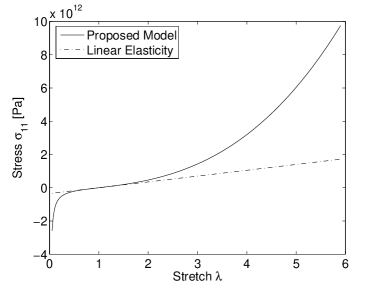
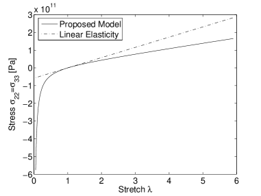
Figure 1: Model response to simple stretch

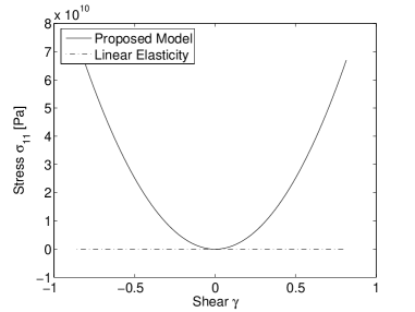
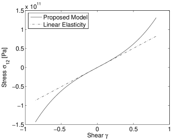
Figure 2: Model response to simple shear

7 Variational formulation and finite element discretization

Consider a body $\mathcal{B}$ with boundary $\partial\mathcal{B}=\mathcal{A}_{1}\cup\mathcal{A}_{2}$. The boundary $\mathcal{A}_{1}$ consists of all surface points where displacement is applied and the boundary $\mathcal{A}_{2}$ of all surface points where tractions are applied ($\mathcal{A}_{1}\cap\mathcal{A}_{2}=\phi$). The boundary value problem can be formulated as (following [17]):

$$\mathrm{Div}(\mathbf{P}) = 0\;\;\;\;\;\;\;\;\;\;\;\;\;\;\;\;\mathrm{in}\;\mathcal{B},$$ (21)

$$\mathbf{P} = \mathbf{P}(\nabla\mathbf{u},\mathbf{x})\;\;\;\mathrm{in}\;\mathcal{B},$$ (22)

$$\mathbf{u} = \mathbf{\bar{u}}\;\;\;\;\;\;\;\;\;\;\;\;\;\;\;\mathrm{on}\;\mathcal{A}_{1},$$ (23)

$$\mathbf{P}\mathbf{n} = \bar{\mathbf{t}}\;\;\;\;\;\;\;\;\;\;\;\;\;\;\;\;\mathrm{on}\;\mathcal{A}_{2},$$ (24)

where (21) expresses the equilibrium condition of the solid in the absence of body forces, (22) is the constitutive law for the solid, (23) expresses the boundary condition for the section of the boundary $\mathcal{A}_{1}$ on which displacement is imposed and (24) refers to the section of the boundary $\mathcal{A}_{2}$ on which the tractions are imposed. For hyperelastic materials possessing strain energy function $\psi$ the first Piola-Kirchhoff stress tensor is given by $\mathbf{P}=\frac{\partial\psi}{\partial\mathbf{F}}$ where $\mathbf{F}=\nabla\mathbf{u}$.

It can be shown ([17]) that the solution $\mathbf{u}$ of the problem posed by (21-24) in the case of polyconvex strain energy function $\psi$ is the minimizer of the functional

$$J(\mathbf{u})=\int_{\mathcal{B}}\psi(\mathbf{x},\mathbf{u},\nabla\mathbf{u})dV-\int_{\partial\mathcal{A}_{2}}\mathbf{u}\cdot\bar{\mathbf{t}}dS,$$ (25)

which can be used to formulate the finite element discretization. The spatial discretization is accomplished by representing the body $\mathcal{B}$ as a union of disjoint elements, $\mathcal{B}=\bigcup_{e=1}^{N_{elem}}\Omega_{e}$. Even though many different elements can be used for the discretization, for simplicity, we will assume that the discretization has been achieved by the use of second order tetrahedral elements. The unknowns to be solved for are the nodal displacements $\mathbf{u}_{n}$. For each element, the displacement is expressed as a sum of the nodal functions, $\mathbf{u}^{(e)}=\sum_{a=1}^{10}N_{a}^{(e)}\mathbf{u}_{a}^{(e)}$. The global displacement approximation becomes $\mathbf{u}_{h}=\sum_{e=1}^{N_{elem}}\sum_{a=1}^{10}N_{a}^{(e)}\mathbf{u}_{a}^{(e)}$. Substitution of $\mathbf{u}_{h}$ into (25) leads to a discrete functional $J_{h}(\mathbf{u}_{h})$. The minimization procedure for the discrete functional gives rise to a system of equations which can be solved for the nodal displacement. Further details about the finite element procedure can be found in [18].

8 Numerical examples

In this section we will consider two basic examples which illustrate the agreement of the model with linear theory at small strains and the departure from it at large deformations.

8.1 2D Example – Plate with Hole

To verify the consistency of our model with linear theory and to check its convergence we considered the problem of uniaxial stress applied to a plate with initially circular hole. In addition to the well known analytical solution for isotropic linear elastic material, this problem has analytic solution for orthotropic linear elastic materials [19]. The stress concentration factor, calculated from this solution specialized to cubic anisotropy with one symmetry axis perpendicular to the plane of the plate and another symmetry axis aligned with the loading direction, is shown on the left side of Figure 3. The numerical solution obtained from our model is in good agreement with this analytical solution when the applied stress is small compared to the elastic constants of the material. As the stress is increased to become comparable to the elastic constants the nonlinearities become important and approximately the same reduction in the minimum and the maximum stress concentration is observed.

The plot on the right of Figure 3 shows the dependence of the error on the mesh size. Within the linear regime the convergence is quadratic as expected for Newton-Raphson solvers. The convergence is somewhat reduced for the nonlinear regime, but it is still within acceptable levels.

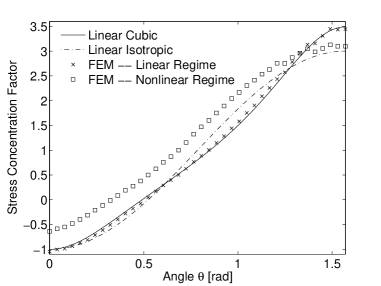
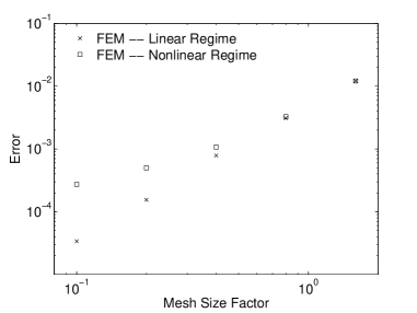
Figure 3: Stress concentration and convergence plots for plate with an initially circular hole

8.2 3D Example – Circular Bar

The problem which we will consider here is the extension of a single crystal cylindrical bar. The bottom end of the bar is clamped and the side surface of the bar is traction free. The top end is displaced in the axial direction by a specified amount, but it is left free to move in the plane perpendicular to the original bar axis. Three different orientations of the bar axis relative to the crystal will be considered. In each case the bar axis will coincide with one of the following crystallographic directions: [100], [110] and [122]. Top and side views of the deformed bar for the three cases are shown in Figure 4. For better visualization the applied displacement is equal to $100$% of the bar length, but the behavior is similar at smaller stretches.

In the first case the cross-section of the bar remains approximately circular and the extension process is approximately symmetric about the bar axis. Similar behavior is observed if the bar axis is aligned with the [111] direction.

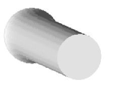
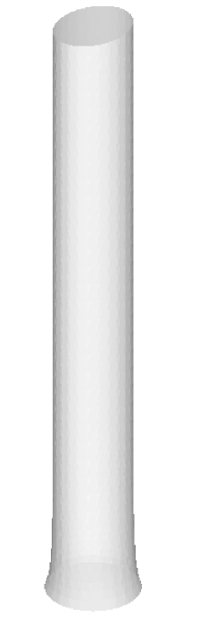
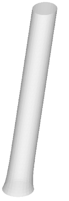
       [100]                [110]                 [122]

Figure 4: Response of single crystal bar to imposed displacement at different orientations of the crystal relative to the bar axis

The anisotropic response is clearly observed in the second case. The contraction of cross-section of the bar in the two directions is markedly different due to the anisotropy brought by the term containing $I_{4}$. As it could be expected the contraction in the [001] direction is much less than in the [$1\bar{1}0$] direction. A possible interpretation of this effect for metallic lattices is that part of the contraction in the latter direction is accomplished by atomic bond rotation rather than pure extension/contraction of the bonds.

The third case illustrates the development of transverse displacements when the crystal lattice lacks enough symmetries relative to the loading axis. The tilting effect is completely due to the anisotropy. If the movement of the top end is restricted significant transverse stresses will develop.

9 Conclusions

A new model for materials with cubic anisotropy has been proposed in this paper. The model is based on additively decoupled strain energy function which satisfy the polyconvexity condition and therefore guarantees existence of minimizing sequences for the appropriate variational functionals. The polyconvexity of new strain energy terms capturing the anisotropy of cubically symmetric systems has been shown. A simple strain energy function capable of capturing the fundamental effect of the anisotropy ratio has been suggested and tested in numerical simulations which reveal that the model possesses many of the relevant physically desirable properties.

The main difference between this model and the orthotropic models in the literature (for example, [1]) is the use of a single fourth order structural tensor. In spite of the complications coming from the higher order of the tensor, the model avoids a major complication which the orthotropic models face: enforcing the equality of the properties in the three mutually perpendicular symmetry directions.

Appendix A Invariants derivatives

The computation of the stress tensor $\mathbf{S}$ and the tangent tensor $\mathbb{C}$ requires the first and second derivatives of the invariants. Expressions for these derivatives deduced in the reference configuration are given below.

• First derivatives

  $$\frac{\partial I_{1}}{\partial C_{IJ}} = \delta_{IJ}$$

  $$\frac{\partial I_{2}}{\partial C_{IJ}} = I_{1}\delta_{IJ}-C_{IJ}$$

  $$\frac{\partial I_{3}}{\partial C_{IJ}} = I_{3}C_{IJ}^{-1}$$

  $$\frac{\partial I_{4}}{\partial C_{IJ}} = {\displaystyle\frac{1}{2}}\left(M_{IJPQ}+M_{JIPQ}+M_{PQIJ}+M_{PQJI}\right)C_{PQ}$$

  $$\frac{\partial I_{5}}{\partial C_{IJ}} = \frac{1}{2}\left[\left(\delta_{IM}\delta_{JN}+\delta_{IN}\delta_{JM}\right)M_{MNPQ}C_{PQ}^{2}+\right.$$

  $$\left.C_{MN}M_{MNPQ}\left(\delta_{IP}C_{JQ}+C_{IQ}\delta_{JP}+C_{PI}\delta_{QJ}+\delta_{IQ}C_{JP}\right)\right]$$

  $$\frac{\partial I_{6}}{\partial C_{IJ}} = \frac{1}{2}\left[\left(\delta_{IM}C_{JN}+\delta_{JM}C_{IN}+C_{IM}\delta_{JN}+C_{JM}\delta_{IN}\right)M_{MNPQ}C_{PQ}^{2}+\right.$$

  $$\left.C_{MN}^{2}M_{MNPQ}\left(\delta_{IP}C_{JQ}+C_{IQ}\delta_{JP}+C_{PI}\delta_{QJ}+\delta_{IQ}C_{JP}\right)\right]$$

  $$\frac{\partial\bar{I}_{M}}{\partial C_{IJ}} = \frac{1}{2}\delta_{MN}M_{MNPQ}\left(\delta_{PI}\delta_{QJ}+\delta_{PJ}\delta_{QI}\right)$$

  $$\frac{\partial\bar{\bar{I}}_{M}}{\partial C_{IJ}} = \frac{1}{2}\delta_{MN}M_{MNPQ}\left(\delta_{PI}C_{QJ}+\delta_{PJ}C_{QI}+C_{PI}\delta_{QJ}+C_{PJ}\delta_{QI}\right)$$

  $$\frac{\partial\hat{I}_{M}}{\partial C_{IJ}} = \frac{1}{2}I_{3}\delta_{MN}M_{MNPQ}\left(2C_{PQ}^{-1}C_{IJ}^{-1}-C_{PI}^{-1}C_{QJ}^{-1}-C_{PJ}^{-1}C_{QI}^{-1}\right)$$

  $$\left(M_{KLJP}+M_{LKJP}\right)C_{PI}+\left(M_{KLPJ}+M_{LKPJ}\right)C_{PI}+$$

  $$C_{PQ}\left(M_{PQIL}\delta_{JK}+M_{PQIK}\delta_{JL}\right)+$$

• Second derivatives

  $$\frac{\partial^{2}I_{1}}{\partial C_{IJ}\partial C_{KL}} = 0$$

  $$\frac{\partial^{2}I_{2}}{\partial C_{IJ}\partial C_{KL}} = \delta_{IJ}\delta_{KL}-\frac{1}{2}\left(\delta_{IK}\delta_{JL}+\delta_{IL}\delta_{JK}\right)$$

  $$\frac{\partial^{2}I_{3}}{\partial C_{IJ}\partial C_{KL}} = I_{3}\left[C_{IJ}^{-1}C_{KL}^{-1}-\frac{1}{2}\left(C_{IK}^{-1}C_{JL}^{-1}+C_{IL}^{-1}C_{JK}^{-1}\right)\right]$$

  $$\frac{\partial^{2}I_{4}}{\partial C_{IJ}\partial C_{KL}} = \frac{1}{4}\left[M_{IJKL}+M_{JIKL}+M_{IJLK}+M_{JILK}+\right.$$

  $$\left.M_{KLIJ}+M_{KLJI}+M_{LKIJ}+M_{LKJI}\right]$$

  $$\frac{\partial^{2}I_{5}}{\partial C_{IJ}\partial C_{KL}} = \frac{1}{4}\left[\left(M_{IJKP}+M_{JIKP}\right)C_{PL}+\left(M_{IJPK}+M_{JIPK}\right)C_{PL}+\right.$$

  $$\left(M_{IJPL}+M_{JIPL}\right)C_{PK}+\left(M_{IJLP}+M_{JILP}\right)C_{PK}+$$

  $$\left(M_{KLIP}+M_{LKIP}\right)C_{PJ}+\left(M_{KLPI}+M_{LKPI}\right)C_{PJ}+$$

  $$\left(M_{KLJP}+M_{LKJP}\right)C_{PI}+\left(M_{KLPJ}+M_{LKPJ}\right)C_{PI}+$$

  $$C_{PQ}\left(M_{PQIL}\delta_{JK}+M_{PQIK}\delta_{JL}\right)+C_{PQ}\left(M_{PQIL}\delta_{JK}+M_{PQIK}\delta_{JL}\right)+$$

  $$C_{PQ}\left(M_{PQIL}\delta_{JK}+M_{PQIK}\delta_{JL}\right)+\left.C_{PQ}\left(M_{PQKI}\delta_{JL}+M_{PQLI}\delta_{JK}\right)\right]$$

  $$\frac{\partial^{2}I_{6}}{\partial C_{IJ}\partial C_{KL}} = \frac{1}{4}\left[\left(M_{ILPQ}\delta_{JK}+M_{IKPQ}\delta_{JL}+M_{JLPQ}\delta_{IK}+M_{JKPQ}\delta_{IL}+\right.\right.$$

  $$\left.+M_{KJPQ}\delta_{IL}M_{LJPQ}\delta_{IK}+M_{KIPQ}\delta_{JL}+M_{LIPQ}\delta_{JK}\right)C_{PQ}^{2}+$$

  $$C_{LP}\left(M_{KPIQ}C_{JQ}+M_{KPJQ}C_{QI}+M_{KPQJ}C_{QI}+M_{KPQI}C_{QJ}\right)+$$

  $$C_{LP}\left(M_{PKIQ}C_{JQ}+M_{PKJQ}C_{QI}+M_{PKQJ}C_{QI}+M_{PKQI}C_{QJ}\right)+$$

  $$C_{KP}\left(M_{LPIQ}C_{JQ}+M_{LPJQ}C_{QI}+M_{LPQJ}C_{QI}+M_{LPQI}C_{QJ}\right)+$$

  $$C_{KP}\left(M_{PLIQ}C_{JQ}+M_{PLJQ}C_{QI}+M_{PLQJ}C_{QI}+M_{PLQI}C_{QJ}\right)+$$

  $$C_{PQ}^{2}\left(M_{PQIL}\delta_{JK}+M_{PQIK}\delta_{JL}+M_{PQJL}\delta_{IK}+M_{PQKJ}\delta_{IL}+\right.$$

  $$M_{PQLJ}\delta_{IK}+\left.\left.M_{PQKI}\delta_{JL}+M_{PQLI}\delta_{JK}+M_{PQJK}\delta_{IL}\right)\right]$$

  $$\frac{\partial^{2}\bar{I}_{M}}{\partial C_{IJ}\partial C_{KL}} = 0$$

  $$\frac{\partial^{2}\bar{\bar{I}}_{M}}{\partial C_{IJ}\partial C_{KL}} = \frac{1}{4}\delta_{MN}M_{MNPQ}\left[\delta_{PI}\left(\delta_{QK}\delta_{JL}+\delta_{QL}\delta_{JK}\right)+\delta_{QI}\left(\delta_{PK}\delta_{JL}+\delta_{PL}\delta_{JK}\right)\right.$$

  $$\left.\delta_{PJ}\left(\delta_{IK}\delta_{QL}+\delta_{IL}\delta_{QK}\right)+\delta_{QJ}\left(\delta_{IK}\delta_{PL}+\delta_{IL}\delta_{PK}\right)\right]$$

  $$\frac{\partial^{2}\hat{I}_{M}}{\partial C_{IJ}\partial C_{KL}} = \frac{1}{2}I_{3}\delta_{MN}M_{MNPQ}\left[\left(2C_{IJ}^{-1}C_{PQ}^{-1}-C_{PI}^{-1}C_{QJ}^{-1}-C_{PJ}^{-1}C_{QI}^{-1}\right)C_{KL}^{-1}-\right.$$

  $$C_{PQ}^{-1}\left(C_{IK}^{-1}C_{JL}^{-1}+C_{IL}^{-1}C_{JK}^{-1}\right)-C_{IJ}^{-1}\left(C_{PK}^{-1}C_{QL}^{-1}+C_{PL}^{-1}C_{QK}^{-1}\right)$$

  $$\frac{1}{2}C_{PI}^{-1}\left(C_{QK}^{-1}C_{JL}^{-1}+C_{QL}^{-1}C_{JK}^{-1}\right)+\frac{1}{2}C_{QJ}^{-1}\left(C_{PK}^{-1}C_{IL}^{-1}+C_{PL}^{-1}C_{IK}^{-1}\right)$$

  $$\left.\frac{1}{2}C_{PJ}^{-1}\left(C_{QK}^{-1}C_{IL}^{-1}+C_{QL}^{-1}C_{IK}^{-1}\right)+\frac{1}{2}C_{QI}^{-1}\left(C_{PK}^{-1}C_{JL}^{-1}+C_{PL}^{-1}C_{JK}^{-1}\right)\right]$$

Appendix B Proofs of basic properties

Statement.

$$\begin{array}[]{l}\begin{array}[]{l}\mathbf{H}^{T}\mathbf{F}:{\bf{M}}:\mathbf{F}^{T}\mathbf{H}=\mathbf{H}^{T}\mathbf{F}:{\bf{M}}:\mathbf{H}^{T}\mathbf{F}\end{array}\end{array}$$ (26)

Proof.

Making use of the indicial notation we have

$$\mathbf{H}^{T}\mathbf{F}:{\bf{M}}:\mathbf{F}^{T}\mathbf{H}=H_{MI}F_{MJ}M_{IJKL}F_{NK}H_{NL}.$$

Considering the symmetries of ${\bf{M}}$, expression (8), and redefining properly dummy indices, the above expression can be rewritten as

$$\begin{array}[]{l}\mathbf{H}^{T}\mathbf{F}:{\bf{M}}:\mathbf{F}^{T}\mathbf{H}=H_{MI}F_{MJ}M_{IJLK}F_{NK}H_{NL}=H_{MI}F_{MJ}M_{IJLK}H_{NL}F_{NK}\\ \qquad\qquad\qquad\quad\,\,\,=\mathbf{H}^{T}\mathbf{F}:{\bf{M}}:\mathbf{H}^{T}\mathbf{F}.\Box\end{array}$$

Statement.

$$\begin{array}[]{l}\begin{array}[]{l}\mathbf{F}^{T}\mathbf{H}:{\bf{M}}:\mathbf{H}^{T}\mathbf{F}=\mathbf{H}^{T}\mathbf{F}:{\bf{M}}:\mathbf{H}^{T}\mathbf{F}\end{array}\end{array}$$ (27)

Proof.

Analogously to the previous statement, we have

$$\begin{array}[]{l}\mathbf{F}^{T}\mathbf{H}:{\bf{M}}:\mathbf{H}^{T}\mathbf{F}=F_{MI}H_{MJ}M_{IJKL}H_{NK}F_{NL}=F_{MI}H_{MJ}M_{JIKL}F_{NK}H_{NL}\\ \qquad\qquad\qquad\quad\,\,\,=H_{MJ}F_{MI}M_{JIKL}H_{NK}F_{NL}=\mathbf{H}^{T}\mathbf{F}:{\bf{M}}:\mathbf{H}^{T}\mathbf{F}.\Box\end{array}$$

Statement.

$$\begin{array}[]{l}\begin{array}[]{l}\mathbf{H}^{T}\mathbf{H}:{\bf{M}}:\mathbf{F}^{T}\mathbf{F}=\mathbf{F}^{T}\mathbf{F}:{\bf{M}}:\mathbf{H}^{T}\mathbf{H}\end{array}\end{array}$$ (28)

Proof.

Similarly to the two statements above, we have

$$\begin{array}[]{l}\mathbf{H}^{T}\mathbf{H}:{\bf{M}}:\mathbf{F}^{T}\mathbf{F}=H_{MI}H_{MJ}M_{IJKL}F_{NK}F_{NL}=F_{NK}F_{NL}M_{IJKL}H_{MI}H_{MJ}\\ \qquad\qquad\qquad\quad\,\,\,=F_{NK}F_{NL}M_{KLIJ}H_{MK}H_{ML}=\mathbf{F}^{T}\mathbf{F}:{\bf{M}}:\mathbf{H}^{T}\mathbf{H}.\Box\end{array}$$

Statement.

If $\mathbf{e}$ is a vector and $\mathbf{A}$, $\mathbf{B}$ and $\mathbf{C}$ are second order tensors then

$$\mathbf{A}:\mathbf{B}\otimes\mathbf{B}:\mathbf{C} = (\mathbf{A}:\mathbf{B})(\mathbf{B}:\mathbf{C})\;\;\;\mathrm{and}$$ (29)

$$\mathbf{e}\otimes\mathbf{e}:\mathbf{A}^{T}\mathbf{A} = (\mathbf{A}\mathbf{e})^{2}.$$ (30)

Proof.

Using index notation, we have the following equalities:

$$\mathbf{A}:\mathbf{B}\otimes\mathbf{B}:\mathbf{C}=A_{IJ}B_{IJ}B_{KL}C_{KL}=(\mathbf{A}:\mathbf{B})(\mathbf{B}:\mathbf{C})$$

and

$$\mathbf{e}\otimes\mathbf{e}:\mathbf{A}^{T}\mathbf{A}=e_{I}e_{J}A_{KI}A_{KJ}=A_{KI}e_{I}A_{KJ}e_{J}=(\mathbf{A}\mathbf{e})^{2}.\Box$$

Statement.

If $\alpha>0$ and $p\geq 2$ satisfy the condition

$$\frac{\alpha+1}{\alpha}\geq\frac{p}{p-1},$$ (31)

then the function $\phi(x,y)=\frac{x^{p}}{y^{\alpha}}$ is convex when considered as a function of both arguments simultaneously.

Proof.

The complete proof is given in [1]. We will only note here that the condition (31) is equivalent to the positive definiteness of the second derivative (the Hessian) of $\phi$. $\Box$

Appendix C Characteristic polynomial

The characteristic polynomial, also known as Cayley-Hamilton polynomial, for a matrix ${\bf{C}}\in M^{3\mathrm{x}3}$, is the equation resulting from the eigenvalue problem corresponding to that matrix ${\bf{C}}$, i.e., $\mathrm{det}(\lambda{\bf{1}-{\bf{C}}})=0$, giving

$$0=\lambda^{3}-\mathrm{tr}({\bf{C}})\lambda^{2}+\mathrm{tr}(\mathrm{adj}({\bf{C}}))\lambda-\mathrm{det}({\bf{C}}),$$

or equivalently

$$0={\bf{C}}^{3}-\mathrm{tr}({\bf{C}}){\bf{C}}^{2}+\mathrm{tr}(\mathrm{adj}({\bf{C}})){\bf{C}}-\mathrm{det}({\bf{C}}){\bf{1}}.$$ (32)

References

- [1] J. Schroder, P. Neff, Invariant formulation of hyperelastic transverse isotropy based on polyconvex free energy functions, International Journal of Solids and Structures 40 (2003) 401–445.
- [2] J. Ball, Constitutive inequalities and existence theorems in elasticity, Springer, Lectures Notes in Math., 1977.
- [3] C. Morrey, The strain-energy function for anisotropic elastic materials, Archives of Mechanics and Engineering 135 (1996) 107–1128.
- [4] J. Weiss, B. Maker, S. Gocindjee, The strain-energy function for anisotropic elastic materials, Archives of Mechanics and Engineering 135 (1996) 107–1128.
- [5] H. Weyl, The Classical Groups. Their Invariants and Representation, Princeton Univ. Press, 1946.
- [6] A. Spencer, Continuum Physics, vol. 1. Theory of invariants, Academic Press, New York, 1971.
- [7] J. Boehler, A simple derivation of representations for non-polynomial constitutive equations in some cases of anisotropy, Zeitschrift fur angewandte Mathematik und Mechanik 59 (1979) 157–167.
- [8] J. Boehler, Introduction to the invariant formulation of anisotropic constitutive equations, CISM Course no. 292. Springer-verlag, 1987.
- [9] J. Betten, Formulation of Anisotropic Constitutive Equations, Springer-Verlag, 1987.
- [10] G. Smith, R. Rivlin, The anisotropic tensors, Quarterly of Applied Mathematics 15 (1957) 309–314.
- [11] G. Smith, R. Rivlin, The strain-energy function for anisotropic elastic materials, Archive for Rational Mechanics and Analysis 15 (1958) 93–133.
- [12] Q. Zheng, A. Spencer, Tensors which characterize anisotropies, International Journal of Engineering Science 31 (5) (1993) 679–693.
- [13] J. E. Marsden, T. J. Hughes, Mathematical Foundations of Elasticity, Dover Publications, Inc., New York, 1983.
- [14] C. Truesdell, W. Noll, The Nonlinear Field Theories of Mechanics, Springer Verlag, 1965.
- [15] J. Betten, Integrity basis for a second-order and a fourth-order tensor, International J. Math. and Math. Sci. 5 (1981) 87–96.
- [16] J. Hirth, J. Lothe, Theory of Dislocations, John Wiley and Sons, 1982.
- [17] J. Ball, Convexity conditions and existence theoremsin nonlinear elasticity, Archive for Rational Mechanics and Analysis 63 (1977) 337–403.
- [18] R. Radovitzky, M. Ortiz, Error estimation and adaptive meshning in strongly nonlinear dynamic problems, Computer Methods in Applied Mechanics and Engineering 172 (1999) 203–240.
- [19] A. E. Green, W. Zerna, Theoretical Elasticity, Oxford University Press, 1968.