Short-range coherence of a lattice Bose atom gas in the Mott insulating phase

Abstract

We study the short-range coherence of ultracold lattice Bose gases in the Mott insulating phase. We calculate the visibility of the interference pattern and the results agree quantitatively with the recent experimental measurement (Phys. Rev. Lett. 95, 050404 (2005)). The visibility deviation from the inversely linear dependence on the bare on-site interaction $U_{0}$ is explained both in smaller and larger $U_{0}$. For a smaller $U_{0}$, it comes from a second order correction. For a larger $U_{0}$, except the breakdown of adiabaticity as analyzed by Gerbier et al, there might be another source to cause this deviation, which is the diversity between $U_{0}$ determined by the single atom Wannier function and the effective on site interaction $U_{\rm eff}$ for a multi-occupation per site.

The observation of the Mott insulating phase in ultracold Bose gases in an optical lattice opens a new era to investigate exactly controllable strong-correlated systems jaks ; mott . For a one-component lattice Bose gases, the Bose Hubbard model BH captures the basic physics of the systems jaks . The theoretical studies mostly focused on the sharp phase transition between the superfluid/Mott-insulator mean ; oosten ; num ; dk ; pv ; yu ; lu . This phase transition may play an important role in various quantum information processing schemes quif .

Recently, the residual short-range interference in the insulating phase has been predicted by numerical studies pred . This phase coherence has been observed by a measurement of the visibility of the interference patterngerb . It was found that the visibility is inversely proportional to the on-site interaction strength $U_{0}$ of the Bose Hubbard model in a wide range. In explaining their data, Gerbier et al assumed a small admixture of particle-hole pairs in the ground state of the Mott insulating phase. They showed that the visibility of interference pattern calculated by this ground state may well match the experimental data in a wide intermediate range of $U_{0}$.

There were deviations from the inverse linear power law in both small and large $U$ in the measurement of the visibility. Gerbier et al interpreted the large $U$ deviation is caused by a breakdown of adiabaticity since the ramping time used in the experiment has been close to the tunnelling time. For the deviation in a small $U$, there was no explanation yet new .

In this paper, we will analytically prove the inverse linear power law of the visibility for intermediate $U$ in the zero temperature. Here the words ’intermediate $U$’ (as well as ’small $U$’, ’large $U$’ in this work) mean the magnitude of $U-U_{c}$ is intermediate (small or large), with $U_{c}$ the critical interaction strength of the superfluid/Mott insulator transition. The result is exactly the same as that obtained by Gerbier et al by assuming a small admixture of the particle hole pair in the ground state gerb . We also show the deviation of the visibility from the inverse linear power law in a small $U$ is caused by a second order correction. For the large $U$, we show that, except the explanation by the authors of the experimental work, owing to the multi-occupation per site, the effective on-site interaction $U_{\rm eff}$ which appears in the Bose Hubbard model cpt ; oo ; li is different from $U_{0}$ which was determined by the single atom Wannier function and used to fit the data of the experiment.

We consider a one-component Bose gas in a 3-dimensional optical lattice described by a periodic potential $V_{0}({\vec{r}})$. Although the real experimental system was confined by a trap potential, we here only pay our attention to the homogeneous system. Beginning with the expansion of the boson field operators in a set of localized basis, i.e., $\psi(\vec{r})=\sum_{i}a_{i}w(\vec{r}-\vec{r}_{i})$ and keeping only the lowest vibrational state, one can define an on-site free energy $f=\bar{n}I+U\bar{n}(\bar{n}-1)/2,$ where $\bar{n}$ is the average occupation per site. The on-site energy $I$ and the bare on-site interaction $U$ are defined by $I=\int d\vec{r}w^{*}(\vec{r})[-\frac{\hbar^{2}}{2m}\nabla^{2}+V_{0}(\vec{r})]w(\vec{r})$,

$$U=\frac{4{\pi}a_{s}\hbar^{2}}{m}\int d\vec{r}|w(\vec{r})|^{4}.$$ (1)

This on-site free energy contributes to the chemical potential by $\mu=-\partial f/\partial\bar{n}$ and defines the effective on-site interaction cpt ; oo ; li

$$U_{\rm eff}=\partial^{2}f/\partial\bar{n}^{2}.$$ (2)

For the single occupation per site, $U_{\rm eff}=U=U_{0}$ and the difference appears for $\bar{n}>1$. We will be back to this issue later. The Bose Hubbard model for a homogeneous lattice gases is defined by the following Hamiltonian

$$H=-t\sum_{\langle ij\rangle}a^{\dagger}_{i}a_{j}+\frac{U_{\rm eff}}{2}\sum_{i}a^{\dagger}_{i}a_{i}a^{\dagger}_{i}a_{i}-\mu\sum_{i}a^{\dagger}_{i}a_{i},$$ (3)

where $\langle ij\rangle$ denotes the sum over the nearest neighbor sites and $\mu$ is the chemical potential. The tunnelling amplitude is defined by

$$t_{B,F;ij}=\int d\vec{r}w^{*}(\vec{r}+\vec{r}_{i})[-\frac{\hbar^{2}\nabla^{2}}{2m}+V_{0}(\vec{r})]w(\vec{r}+\vec{r}_{j}),$$

for a pair of the nearest neighbor sites $(i,j)$.

Our main goal is to calculate the interference pattern

$$S(\vec{k})=\sum_{i,j}e^{i\vec{k}\cdot(\vec{r}_{i}-\vec{r}_{j})}\langle a^{\dagger}_{i}a_{j}\rangle,$$ (4)

which is related to the density distribution of the expanding atom clouds by $\rho(\vec{r})=\frac{m}{\hbar t_{ex}}|\tilde{w}(\vec{k}=m\vec{r}/\hbar t_{ex})|^{2}S(\vec{k})$ with $m$ the atom mass and $t_{ex}$ the time of the atom free expansion pred ; pe . Since we are interested in the Mott insulating phase, we can calculate $S(\vec{k})$ by taking the tunnelling term as a perturbation. To do this, we introduce a Hubbard-Stratonovich field in the partition function dk

$$Z[J,J^{*}]=\int{\cal D}\Phi^{*}{\cal D}\Phi{\cal D}a^{*}{\cal D}a\exp\biggl{\{}-S_{0}$$

$$+t\int_{0}^{\beta}d\tau\sum_{\langle ij\rangle}a^{*}_{i}a_{j}+\int_{0}^{\beta}d\tau\sum_{i}(J^{*}_{i}a_{i}+J_{i}a^{*}_{i})$$

$$-t\int_{0}^{\beta}d\tau(a^{*}_{i}-\Phi^{*}_{i}+J^{*}_{i}/t)(a_{j}-\Phi_{j}+J_{j}/t)\biggr{\}},$$ (5)

where $S_{0}$ is the $t$-independent part in the full action and $J$ and $J^{*}$ are currents introduced to calculate correlation functions. Integrating away $a_{i}$ and $a^{*}_{i}$ and transferring into the lattice wave vector and thermal frequency space, one has

$$Z[J^{*},J] = \int{\cal D}\Phi^{*}{\cal D}\Phi\exp\biggl{\{}\sum_{\vec{k},n}(-\Phi_{\vec{k},n}^{*}{\cal G}^{-1}(\vec{k},i\omega_{n})\Phi_{\vec{k},n}$$ (6)

$$+ J^{*}_{\vec{k},n}\Phi_{\vec{k},n}+J_{\vec{k},n}\Phi^{*}_{\vec{k},n}+\frac{1}{\epsilon_{k}}J^{*}_{\vec{k},n}J_{\vec{k},n},$$

where $\epsilon_{k}=-2t\sum_{\nu=x,y,z}\cos k_{\nu}$. The correlation function is calculated in a standard way:

$$\langle a^{*}_{\vec{k},n}a_{\vec{k},n}\rangle=\frac{1}{Z[0,0]}\frac{\delta^{2}Z[J^{*},J]}{\delta J^{*}_{\vec{k},n}\delta J_{\vec{k},n}}\biggr{|}_{J^{*}=J=0}$$

$$=\langle\Phi^{*}_{\vec{k},n}\Phi_{\vec{k},n}\rangle+\frac{1}{\epsilon_{k}}=-{\cal G}(\vec{k},i\omega_{n})+\frac{1}{\epsilon_{k}}.$$ (7)

The interference pattern then may be expressed as

$$S(\vec{k})=-\frac{1}{\beta}\sum_{n}[{\cal G}(\vec{k},i\omega_{n})-\frac{1}{\epsilon_{k}}].$$ (8)

In the Mott insulating phase, the correlation function ${\cal G}(\vec{k},i\omega_{n})$ has been calculated by slave particle techniques dk ; yu

$${\cal G}^{-1}({\bf k},i\omega_{n})=\epsilon_{\bf k}-\epsilon_{\bf k}^{2}\sum_{\alpha=0}^{\infty}(\alpha+1)\frac{n^{\alpha}-n^{\alpha+1}}{i\omega_{n}+\mu-\alpha U},$$ (9)

where the slave particle occupation number is given by

$$n^{\alpha}=\frac{1}{\exp\{\beta[-i\lambda-\alpha\mu+\alpha(\alpha-1)U_{\rm eff}/2]\}\pm 1},$$ (10)

which obeys $\sum_{\alpha}n^{\alpha}=1$ and $\sum_{\alpha}\alpha n^{\alpha}=N$ in the mean field approximation note . $\lambda$ is a Lagrangian multiplier to ensure $\sum_{\alpha}n^{\alpha}=1$. The sign $\pm$ corresponds to the slave fermion or boson, respectively. In previous works, we have show that the slave fermion approach may have some advantages to the slave boson approachyu ; lu . We then take the slave fermion formalism. In the Mott insulating phase, since $U_{\rm eff},\mu\gg t$, one can expand ${\cal G}(\vec{k},i\omega_{n})$ in terms of $\epsilon_{k}/(i\omega_{n}-\mu+\alpha U_{\rm eff})$ and the interference pattern reads

$$S(\vec{k}) = -\frac{1}{\beta}\sum_{n}({\cal G}(\vec{k},\omega_{n})-\frac{1}{\epsilon_{k}})$$ (11)

$$= \frac{1}{\beta}\sum_{n}\sum_{a=0}(-1)^{a}\epsilon_{k}^{a}(A(\omega_{n}))^{a+1},$$

$$A(\omega_{n}) = \sum_{\alpha=0}^{\infty}(\alpha+1)\frac{n^{\alpha+1}-n^{\alpha}}{i\omega_{n}+\mu-\alpha U_{\rm eff}}.$$

Making the frequency sum, one has, to the first order of $\epsilon_{k}$,

$$S(\vec{k}) \approx -\sum_{\alpha}n_{B}(\alpha U_{\rm eff}-\mu)(\alpha+1)(n^{\alpha+1}-n^{\alpha})$$

$$- \epsilon_{k}\beta\sum_{\alpha}[(\alpha+1)^{2}(n^{\alpha+1}-n^{\alpha})^{2}$$

$$\times n_{B}(\alpha U_{\rm eff}-\mu)(1+n_{B}(\alpha U_{\rm eff}-\mu))$$

$$- \frac{2\epsilon_{k}}{U_{\rm eff}}\sum_{\alpha<\gamma}(n_{B}(\alpha U_{\rm eff}-\mu)-n_{B}(\gamma U_{\rm eff}-\mu))$$

$$\times (\alpha+1)(\gamma+1)(n^{\alpha+1}-n^{\alpha})(n^{\gamma+1}-n^{\gamma}),$$

where $n_{B}(\alpha U_{\rm eff}-\mu)=[e^{\beta(\alpha U_{\rm eff}-\mu)}-1]^{-1}$. In the limit $T\to 0$ and the $n_{0}$-th Mott lobe, one knows $(n_{0}-1)U_{\rm eff}<\mu<n_{0}U_{\rm eff}$ and $n^{\alpha}=\delta_{\alpha,n_{0}}$. Substituting these into (Short-range coherence of a lattice Bose atom gas in the Mott insulating phase), one obtains the zero temperature value of $S(\vec{k})$

$$S(\vec{k},T=0)=n_{0}-2n_{0}(n_{0}+1)\frac{\epsilon_{k}}{U}_{\rm eff}.$$ (13)

This is what Gerbier et al obtained by assuming the particle-hole pair admixture in the ground state gerb . Integrating along one lattice direction, the corresponding 2D visibility is given by

$${\cal V}=\frac{\rho_{\rm max}-\rho_{\rm min}}{\rho_{\rm max}+\rho_{\rm min}}=\frac{S_{\rm max}-S_{\rm min}}{S_{\rm max}+S_{\rm min}}\approx\frac{4}{3}(n_{0}+1)\frac{zt}{U}_{\rm eff}$$ (14)

for $z=6$, where $\rho_{\rm max}$ and $\rho_{\rm min}$ are chosen such that the Wannier envelop was cancelled. This is the inverse linear power law used to fit the experimental data gerb . However, the experimental data deviated from this power law fit when $U_{\rm eff}/zt<8$. In terms of (11), we think that this comes from a second order correction. A direct calculation shows that the second order correction in zero temperature is given by note1

$$\delta^{(2)}S(\vec{k})=3n_{0}(n_{0}+1)^{2}\frac{\epsilon_{k}^{2}}{U_{\rm eff}^{2}}.$$ (15)

Thus, the 2D visibility for $n_{0}=1$ is modified to

$${\cal V}=\frac{8}{3\bar{U}_{\rm eff}(1+32\bar{U}_{\rm eff}^{-2}/3)},$$ (16)

with $\bar{U}_{\rm eff}=U_{\rm eff}/zt$. In Fig. 1, we show the visibility against $\bar{U}_{\rm eff}$ in a log-log plot for $n_{0}=1$. This second order correction suppresses the visibility for a small $\bar{U}_{\rm eff}$ while the exponent of the power law seems deviating from $-1$ a little. These features agree with the experimentally measured data.

Figure 1: Visibility of the interference pattern versus $\bar{U}_{\rm eff}$ according to (16) in a log-log plot(the dot line with circles) . The solid line is the inverse linear power law (14) and the dash line is a power law fit with an exponent $-0.95$ to (16).

We have neglected the finite temperature effect to compare with the experiment although our theory is in finite temperature. In fact, there may be a finite temperature correction to the interference pattern in the second order. According to (11), it is given by, near $n_{0}=1$

$$\delta^{(2)}S_{T}(\vec{k})=18(n^{1})^{2}n^{2}\frac{\epsilon^{2}_{k}}{U_{\rm eff}^{2}},$$ (17)

which may further suppresses the visibility. For instance, at $T=1.0zt\sim 10^{1}$nK, the ratio between (17) and (15) is

$$\frac{\delta^{(2)}_{T}S(\vec{k})}{\delta^{(2)}S(\vec{k})}=3(n^{1})^{2}n^{2}/2$$

$$=0.106,0.098,0.087,~{}{\rm and}~{}0.064$$

for $\bar{U}_{\rm eff}=6,7,8,$ and 10. However, the temperature in the Mott insulator is difficult to be estimated in the experiment thank . Thus, a quantitative comparison of the finite temperature calculation to the experiment data is waiting for more experimental developments.

We now discuss the large $U$ deviation from the inverse linear power law, which has been seen in the experiment and explained by the breakdown of adiabaticity gerb . We will reveal another possible source for this deviation. As we have mentioned before, the value of $U_{\rm eff}$ may be different from $U$ and $U_{0}$ for $\bar{n}>1$. Our above calculation showed an inverse linear power law to $U_{\rm eff}$ whereas the experimentalists used $U_{0}$ to fit their data.

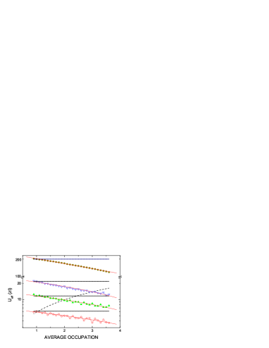
Figure 2: (Color online) The effective on-site interaction $U_{\rm eff}$ versus the average occupation per site, $\bar{n}$ in a $\bar{n}$-$\log(U_{\rm eff})$ plot. The thin solid lines are linear fits to variational data for $V_{0}=11.95,14.32$, 16.25 and 29 $E_{R}$ (empty circles, filled triangles, empty triangles and filled circles, respectively). The dash line is critical interaction strength calculated by the mean field theory mean ; oosten . The thick horizontal lines are the on-site interactions $U_{0}$ calculated by the single atom Warrier function.

Due to the interaction, the atom energy band may be modified and the Wannier function may be broadened, compared to the single atom ones. In Ref. li , we have considered the mean field interaction and made a variational calculation to the Wannier function by using Kohn’s method kohn . The direct result of the broadening of the Wannier function is the bare on-site interaction $U$ becomes weaker than $U_{0}$ which is calculated by the single atom Wannier function. The $\bar{n}$-dependence of $I$ may further reduce $U_{\rm eff}$ from $U$. In Fig. 2, we plot $U_{\rm eff}$ versus $\bar{n}$. In the low part of Fig. 2, three typical lattice depths are considered, $V_{0}=11.95,14.32$ and 16.25 $E_{R}(=\frac{\hbar^{2}k^{2}}{2m})$, corresponding to the critical interaction strengths of the $n_{0}=1,2$ and 3 Mott states. The up-part is for $V_{0}=29E_{R}$, which was the lattice depth where the adiabaticity breaks gerb .

Several points may be seen from Fig. 2. First, the critical values of $V_{0}=14.32E_{R}$ for $n_{0}=2$ and $16.25E_{R}$ for $n_{0}=3$ are closer to experimental ones, 14.1(8) $E_{R}$ and 16.6(9) $E_{R}$ gerb , comparing to 14.7 $E_{R}$ and 15.9$E_{R}$, corresponding to the single atom Wannier functions. Second, the variational data are downward as $\bar{n}$ indicates that $-\log U_{\rm eff}>-\log U_{0}$ for $\bar{n}>1$. This may cause two results: (a) If $-\log U_{\rm eff}$ deviates from $-\log U_{0}$ a small magnitude, the power law fit presents an exponents $-(1-\delta)$. This has been observed in experiment, which is $-0.98(7)$ gerb . (b) As $\bar{n}$ increases, the deviation becomes significant. This may appear in a large $V_{0}$. In the experiment, the latter appeared in $V_{0}>29E_{R}$. We show that, in Fig. 2, the deviation is not a small magnitude for $V_{0}=29E_{R}$.

In summary, we studied the short-range coherence in the Mott insulating phase with a finite on-site interaction strength. The interference pattern and then its visibility were calculated by using a perturbation theory. The inverse linear power law of the visibility to the interaction strength, which was found in the experiment, was exactly recovered. We further discussed the deviation from this power law both in a small and large $U_{0}$. We found that a second order effect suppresses the visibility for a small $U_{0}$ while its up-deviation in a large $U_{0}$ might be caused by the difference between $U_{0}$ and $U_{\rm eff}$ except the possible breakdown of adiabaticity.

We would like to thank Fabrice Gerbier for useful discussions. This work was supported in part by the National Natural Science Foundation of China.

References

• (1) D. Jaksch, C. Bruder, J. I. Cirac, C. W. Gardiner and P. Zoller, Phys. Rev. Lett. 81, 3108 (1998).
• (2) M. Greiner, O. Mandel, T. Esslinger, T. W. HΓ€nsch and I. Bloch, Nature 415, 39 (2002). T. StΓΆferle, H. Moritz, C. Schori, M. KΓΆhl, T. Esslinger, Phys. Rev. Lett. 92, 130403(2004).
• (3) M. P. A. Fisher, P. B. Weichman, G. Grinstein, and D. S. Fisher, Phys. Rev. B 40, 546 (1989).
• (4) W. Krauth, M. Caffarel, and J. P. Bouchard, Phys. Rev. B 45, 3137 (1992); K. Sheshadri et al., Europhys. Lett. 22, 257 (1993); J. K. Freericks and H. Monien, Europhys. Lett. 26, 545 (1994).
• (5) D. van Oosten, P. van der Straten, and H. T. C. Stoof, Phys. Rev. A 63, 053601 (2001).
• (6) G. G. Batrouni, V. Rousseau, R. T. Scalettar, M. Rigol, A. Muramatsu, P. J. H. Denteneer, and M. Troyer, Phys. Rev. Lett. 89, 117203 (2002). G. G. Batrouni, R. T. Scalettar, and G. T. Zimanyi, Phys. Rev. Lett. 65, 1765 (1990). S. Wessel, F. Alet, M. Troyer, and G. G. Batrouni, Phys. Rev. A 70, 053615 (2004).
• (7) D. B. Dickerscheid, D. van Oosten, P. J. H. Densteneer, and H. T. C. Stoof, Phys. Rev. A 68, 043623(2003).
• (8) P. Buonsante and A. Vezzani, Phys. Rev. A 70, 033608 (2004).
• (9) Yue Yu and S. T. Chui, Phys. Rev. A 71, 033608(2005).
• (10) X. C. Lu, J. B. Li, and Y. Yu, cond-mat/0504503.
• (11) P. Rabl, A. J. Daley, P. O. Fedichev, J. I. Cirac, and P. Zoller, Phys. Rev. Lett. 91, 110403 (2003). G. Pupillo, A. M. Rey, G. K. Brennen, C. W. Clark, and C. J. Williams, Journal of Modern Optics 51, 2395 (2004). B. DeMarco, C. Lannert, S. Vishveshwara, and T.-C. Wei, cond-mat/0501718 (2005).
• (12) V. A. Kashurnikov, N. V. Prokof ev, and B. V. Svistunov, Phys. Rev. A 66, 031601(R) (2002). R. Roth and K. Burnett, Phys. Rev. A 67, 031602(R) (2003). C. Schroll, F. Marquardt and C. Bruder, Phys. Rev. A 70, 053609 (2004).
• (13) F. Gerbier, A. Widera, S. FΓΆlling, O. Mandel, T. Gericke, and I. Bloch, Phys. Rev. Lett. 95, 050404 (2005).
• (14) After this paper was submitted, there were two works concerning this issue. See, F. Gerbier, A. Widera, S. FΓΆlling, O. Mandel, T. Gericke, and I. Bloch, arXiv.org:cond-mat/0507087; E. Calzetta, B-L Hu, A. M. Rey, arXiv.org:cond-mat/0507256.
• (15) M. L. Chiofalo, M. Polini, and M. P. Tosi, Euro. Phys. J. D 11, 371 (2000).
• (16) D. van Oosten, P. van der Straten, and H. T. C. Stoof, Phys. Rev. A 67, 033606 (2003).
• (17) Jinbin Li, Yue Yu, A. Dudarev and Qian Niu , cond-mat/0311012.
• (18) P. Pedri, L. Pitaevskii, S. Stringari, C. Fort, S. Burger, F. S. Cataliotti, P. Maddaloni, F. Minardi, and M. Inguscio, Phys. Rev. Lett. 87, 220401 (2001).
• (19) We do not consider the fluctuations to these two equations.
• (20) There is also a correction $\delta^{(2)}S\propto\bar{U}_{\rm eff}^{-2}$ for $n_{0}>1$ in principle. However, this corresponds to a much larger $\bar{U}_{\rm eff}$ and therefore, may become not visible in experiments.
• (21) W. Kohn, Phys. Rev. B 7, 4388 (1973).
• (22) We thank Fabrice Gerbier told us this point.