Determination of the phase shifts for interacting electrons connected to reservoirs

Abstract

We describe a formulation to deduce the phase shifts, which determine the ground-state properties of interacting quantum-dot systems with the inversion symmetry, from the fixed-point eigenvalues of the numerical renormalization group (NRG). Our approach does not assume the specific form of the Hamiltonian nor the electron-hole symmetry, and it is applicable to a wide class of quantum impurities connected to noninteracting leads. We apply the method to a triple dot which is described by a three-site Hubbard chain connected to two noninteracting leads, and calculate the dc conductance away from half-filling. The conductance shows the typical Kondo plateaus of the Unitary limit $g\simeq 2e^{2}/h$ in some regions of the onsite energy $\epsilon_{d}$, at which the total number of electrons $N_{\rm el}$ in the three dots is odd, i.e., $N_{\rm el}\simeq 1$, $3$ and $5$. In contrast, the conductance shows a wide minimum in the regions of $\epsilon_{d}$ corresponding to even number of electrons $N_{\rm el}\simeq 2$ and $4$. We also discuss the parallel conductance of the triple dot connected transversely to four leads, and show that it can be deduced from the two phase shifts defined in the two-lead case.

1 Introduction

The Kondo effect in quantum dots is a subject of much current interest, [1, 2] and experimental developments in this decade make it possible to examine the interplay of various effects which have previously only been studied in different fields of physics.[3, 4] For instance, in quantum dots, the interplay of the Aharanov-Bohm, Fano, Josephson, and Kondo effects under equilibrium and nonequilibrium situations have been studied intensively.[5, 6, 7]

To study the low-temperatures properties of the systems showing the Kondo behavior, reliable theoretical approaches are required. The Wilson numerical renormalization group (NRG) method [8, 9, 10] has been used successfully for single and double quantum dots.[11, 12] In a previous work, we have applied the NRG method to a finite Hubbard chain of finite size $N_{C}$ connected to noninteracting leads, and have studied the ground-state properties at half-filling. [13] The results obtained for $N_{C}=3$ and $4$ show that the low-lying eigenstates have one-to-one correspondence with the free quasi-particle excitations of a local Fermi liquid. It enables us to determine the transport coefficients from the fixed-point Hamiltonian. Furthermore, it enables us to deduce the characteristic parameters such as $T_{K}$ and Wilson ratio $R$ from the fixed-point eigenvalues, and the calculations have been carried out for the Anderson impurity model. [14, 15] The purpose of this paper is to provide an extended formulation to deduce the conductance away from half-filling.

The ground-state properties of quantum dots connected to two noninteracting leads are determined by the two phase shifts if the systems have an inversion symmetry. Kawabata described the outline of this feature assuming that the low-energy properties are determined by the quasi-particles of a local Fermi liquid,[16] and discussed qualitatively the role of the Kondo resonance on the tunneling through a quantum dot. In this paper we describe the formulation to deduce these two phase shifts from the fixed-point eigenvalues of NRG. The formulation along these lines is well known for some particular cases, and has been applied to the single and double quantum dots. [5, 11, 12] However, to our knowledge, a general description has not been given explicitly so far. Our formulation does not assume a specific form of the Hamiltonian, and thus it is applicable to a wide class of the models for quantum impurities. We apply the method to a three-site Hubbard chain. It is a model for a triple dot, and the low-energy properties of this system away from half-filling have not been clarified with reliable methods yet. We calculate the dc conductance $g$ away from half-filling as a function of the onsite energy $\epsilon_{d}$ which can be controlled by the gate voltage. The results show the typical Kondo plateaus of the Unitary limit $g\simeq 2e^{2}/h$ when the average number of electrons $N_{\rm el}$ in the chain is odd, $N_{\rm el}\simeq 1$, $3$, and $5$. In contrast, for some finite ranges of $\epsilon_{d}$ corresponding to even number of electrons $N_{\rm el}\simeq 2$ and $4$, the conductance shows wide minima. We also discuss the parallel conductance of the triple dot connected transversely to four leads.

In §2, we introduce a model for interacting electrons connected to reservoirs in a general form, and describe the ground-state properties in terms of the phase shifts. In §3, we describe the formulation to deduce the phase shifts from the fixed-point Hamiltonian of NRG. In §4, we apply the formulation to the transport through the triple dot. In §5, discussion and summary are given.

2 Model and Formulation

We start with a system consisting of a finite central region ($C$) and two leads, on the left ($L$) and the right ($R$), as illustrated in Fig. 1. The central region consists of $N_{C}$ quantized levels, and the interaction $U_{j_{4}j_{3};j_{2}j_{1}}$ is switched on for the electrons staying in this region. Each of the two leads has a continuous energy spectrum. The complete Hamiltonian is given by

$${\cal H} \,=\,{\cal H}_{C}^{0}\,+\,{\cal H}_{C}^{U}+\,{\cal H}_{\rm mix}\,+\,{\cal H}_{\rm lead}\;,$$ (1)

$${\cal H}_{C}^{0} \,=\,-\sum_{ij\in C,\sigma}t_{ij}^{\phantom{0}}\,d^{\dagger}_{i\sigma}d^{\phantom{\dagger}}_{j\sigma}$$ (2)

$${\cal H}_{C}^{U} \,=\,{1\over 2}\sum_{\{j\}\in C}\sum_{\sigma\sigma^{\prime}}U_{j_{4}j_{3};j_{2}j_{1}}\,d^{\dagger}_{j_{4}\sigma}d^{\dagger}_{j_{3}\sigma^{\prime}}d^{\phantom{\dagger}}_{j_{2}\sigma^{\prime}}d^{\phantom{\dagger}}_{j_{1}\sigma}$$ (3)

$${\cal H}_{\rm mix}\, \,=\,v_{L}^{\phantom{0}}\sum_{\sigma}\left(\,d^{\dagger}_{1,\sigma}\psi^{\phantom{\dagger}}_{L\sigma}\,+\,\psi^{\dagger}_{L\sigma}d^{\phantom{\dagger}}_{1,\sigma}\,\right)$$

$$\ \ +v_{R}^{\phantom{0}}\sum_{\sigma}\left(\,\psi^{\dagger}_{R\sigma}d^{\phantom{\dagger}}_{N_{C},\sigma}\,+\,d^{\dagger}_{N_{C},\sigma}\psi^{\phantom{\dagger}}_{R\sigma}\,\right),$$ (4)

$${\cal H}_{\rm lead} \,=\,\sum_{\nu=L,R}\sum_{k\sigma}\epsilon_{k\nu}^{\phantom{0}}\,c^{\dagger}_{k\nu\sigma}c^{\phantom{\dagger}}_{k\nu\sigma}\,,$$ (5)

where $d_{i\sigma}$ annihilates an electron with spin $\sigma$ at site $i$. In the lead at $\nu$ ($=L,\,R$), the operator $c_{k\nu\sigma}^{\dagger}$ creates an electron with energy $\epsilon_{k\nu}$ corresponding to an one-particle state $\phi_{k\nu}(r)$. The tunneling matrix elements $v_{L}^{\phantom{\dagger}}$ and $v_{R}^{\phantom{\dagger}}$ connect the central region and two leads. At the interfaces, a linear combination of the conduction electrons $\psi_{\nu\sigma}^{\phantom{\dagger}}=\sum_{k}c_{k\nu\sigma}^{\phantom{\dagger}}\,\phi_{k\nu}(r_{\nu})$ mixed with the electrons at $i=1$ or $N_{C}$, where $r_{\nu}$ denotes the position at the interface in the lead side. We assume that the hopping matrix elements $t_{ij}$ and $v_{\nu}^{\phantom{\dagger}}$ are real, and the interaction has the time-reversal symmetry: $U_{43;21}$ is real and $U_{43;21}=U_{34;12}=U_{12;34}=U_{42;31}=U_{13;24}$. We will be using units $\hbar=1$ unless otherwise noted.

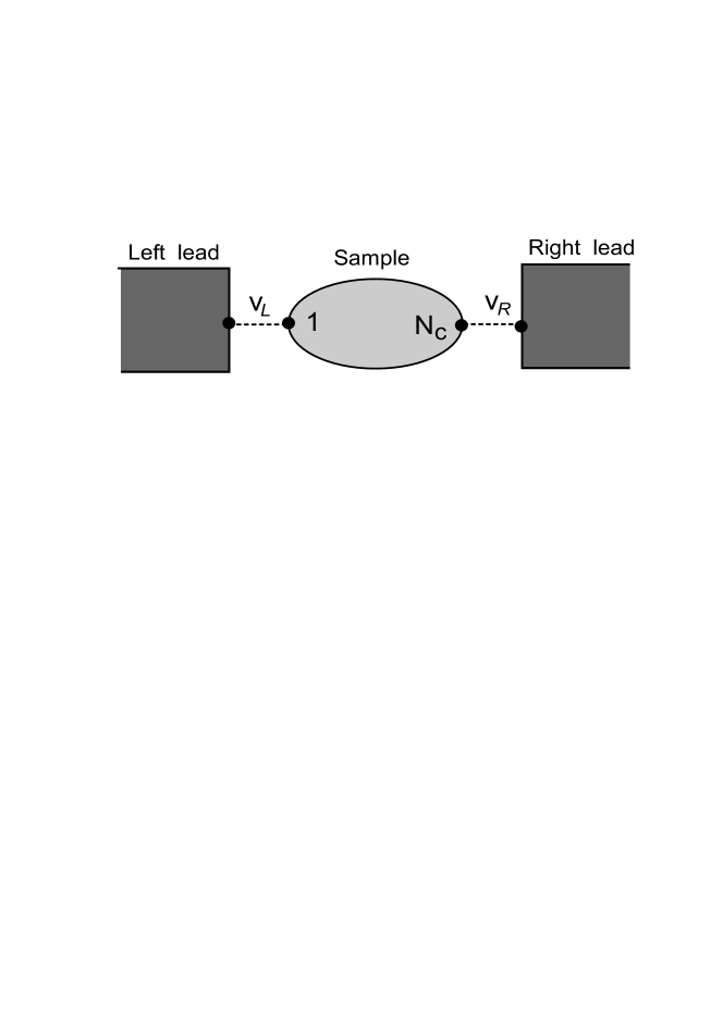
Figure 1: Schematic picture of a series connection

We use the Green’s function for the interacting region ($ij\in C$) defined by

$$G_{ij}(\text{i}\omega_{n})\,=\,-\int_{0}^{\beta}\!\text{d}\tau\,\left\langle T_{\tau}\,d^{\phantom{\dagger}}_{i\sigma}(\tau)\,d^{\dagger}_{j\sigma}(0)\right\rangle\,\text{e}^{\text{i}\omega_{n}\tau}\;,$$ (6)

where $\beta=1/T$, $d_{j\sigma}(\tau)=\text{e}^{\tau{\cal H}}d_{j\sigma}\text{e}^{-\tau{\cal H}}$, and $\langle{\cal O}\rangle=\mbox{Tr}\left[\,\mathrm{e}^{-\beta{\cal H}}\,{\cal O}\,\right]/\mbox{Tr}\,\mathrm{e}^{-\beta{\cal H}}$. The corresponding retarded and advanced functions are given by $G_{ij}^{\pm}(\omega)=G_{ij}(\omega\pm\text{i}\,\delta)$ via the analytic continuation. The Dyson equation for the Green’s function $\mbox{\boldmath$G$}(z)=\{G_{ij}(z)\}$ can be rewritten in an $N_{C}\times N_{C}$ matrix form

$$\left\{\mbox{\boldmath$G$}(z)\right\}^{-1}\,=\,z\,\mbox{\boldmath$1$}-\mbox{\boldmath$H$}_{C}^{0}-\mbox{\boldmath$V$}_{\rm mix}(z)-\mbox{\boldmath$\Sigma$}(z)\;,$$ (7)

where $\mbox{\boldmath$H$}_{C}^{0}=\{-t_{ij}^{\phantom{0}}\}$,

$$\mbox{\boldmath$V$}_{\rm mix}(z) \,=\,\left[\,\begin{matrix}v_{L}^{2}\mbox{\sl g}_{L}^{\phantom{\dagger}}(z)&0&&\mbox{\Large$0$}\cr 0&0&\ \ddots&\cr&\ddots\ &\ddots&0\cr\mbox{\Large$0$}&&0&v_{R}^{2}\mbox{\sl g}_{R}^{\phantom{\dagger}}(z)\cr\end{matrix}\,\right]\;,$$ (8)

and $\mbox{\boldmath$\Sigma$}(z)=\{\Sigma_{ij}(z)\}$ is the self-energy due to the inter-electron interaction ${\cal H}_{C}^{U}$. In the matrix $\mbox{\boldmath$V$}_{\rm mix}(z)$, the two non-zero elements are determined by the Green’s function at interface of the isolated lead $\mbox{\sl g}_{\nu}^{+}(\omega)\equiv\sum_{k}{\left|\phi_{\nu\sigma}^{\phantom{\dagger}}(r_{\nu})\right|^{2}/(\omega-\epsilon_{k\nu}+i0^{+})}$. We assume, for simplicity, that the density of states $\rho_{\nu}$ is a constant for small $\omega$. Then, the energy scale of the level-broadening becomes $\Gamma_{\nu}=\pi\rho_{\nu}v_{\nu}^{2}$, and $\mbox{\sl g}_{\nu}^{+}(\omega)=-\text{i}\pi\rho_{\nu}$.

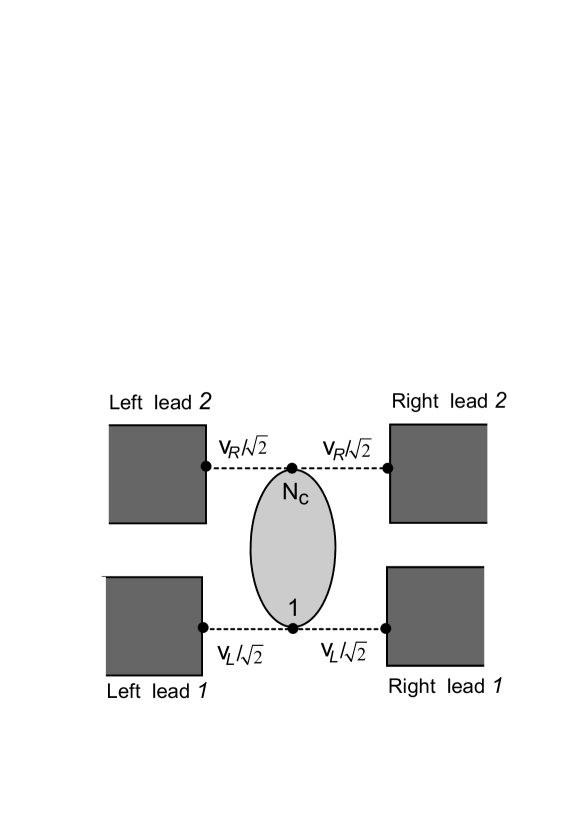
Figure 2: Schematic picture of a parallel connection.

2.1 Ground state properties

If the self-energy shows a property $\mbox{Im}\,\mbox{\boldmath$\Sigma$}^{+}(0)=0$ at $T=0$, then the damping of the single-particle excitations at the Fermi level vanishes. In this case, the renormalization hopping matrix elements $\mbox{\boldmath$H$}_{C}^{\rm eff}=\{-\widetilde{t}_{ij}\,\}$ defined by

$$\mbox{\boldmath$H$}_{C}^{\rm eff}\,\equiv\,\mbox{\boldmath$H$}_{C}^{0}+\mbox{Re}\,\mbox{\boldmath$\Sigma$}^{+}(0)$$ (9)

play a central role on the ground-state properties. The value of the Green’s function at the Fermi level is given by $\left\{\mbox{\boldmath$G$}^{+}(0)\right\}^{-1}=\mbox{\boldmath$K$}(0)-\mbox{\boldmath$V$}_{\rm mix}^{+}(0)$ with

$$\mbox{\boldmath$K$}(\omega)\,\equiv\,\omega\,\mbox{\boldmath$1$}-\mbox{\boldmath$H$}_{C}^{\rm eff}\;,$$ (10)

and the scattering coefficients at $T=0$ are determined by the determinant

$$\det\left\{\mbox{\boldmath$G$}^{+}(0)\right\}^{-1} \,=\,\left[\,-\Gamma_{L}\,\Gamma_{R}\,\det\mbox{\boldmath$K$}_{11}^{N_{C}N_{C}}(0)+\det\mbox{\boldmath$K$}(0)\,\right]\,$$

$$\!\!\!\!\!\!+\,\text{i}\,\Bigl{[}\,\Gamma_{L}\,\det\mbox{\boldmath$K$}_{11}(0)+\Gamma_{R}\,\det\mbox{\boldmath$K$}_{N_{C}N_{C}}(0)\,\Bigr{]}\;.$$ (11)

Here $\mbox{\boldmath$K$}_{ij}(0)$ is an $(N_{C}-1)\times(N_{C}-1)$ derived from $\mbox{\boldmath$K$}(0)$ by deleting the $i$-th row and $j$-th column. Similarly, $\mbox{\boldmath$K$}_{11}^{N_{C}N_{C}}(0)$ is an $(N_{C}-2)\times(N_{C}-2)$ matrix obtained from $\mbox{\boldmath$K$}(0)$ by deleting the first and $N_{C}$-th rows, and the first and $N_{C}$-th columns. The dc conductance at $T=0$ can be expressed, using an inter-boundary Green’s function,[17, 18, 19] as

$$g_{\rm series}^{\phantom{0}}\,=\,\frac{2e^{2}}{h}4\Gamma_{R}\Gamma_{L}\left|G_{N_{C}1}^{+}(0)\right|^{2}\;.$$ (12)

Similarly, at $T=0$ the charge displacement $N_{\rm el}$ caused by the hybridizations $\Gamma_{L}$ and $\Gamma_{R}$ can be expressed, using the Friedel sum rule,[20, 21] as

$$N_{\rm el} \,=\,{1\over\pi\text{i}}\,\log\left[\det\mbox{\boldmath$S$}\right]\;,$$ (13)

$$S \,=\left[\,\begin{matrix}1-2\text{i}\,\Gamma_{L}G_{11}^{+}(0)&\ \ -2\text{i}\,\Gamma_{L}G_{1N_{C}}^{+}(0)\cr-2\text{i}\,\Gamma_{R}G_{N_{C}1}^{+}(0)&\rule{0.0pt}{14.22636pt}\ 1-2\text{i}\,\Gamma_{R}G_{N_{C}N_{C}}^{+}(0)\cr\end{matrix}\,\right]\;.$$ (14)

In the case of the constant density of states we are assuming, the charge displacement coincides with the total number of electrons in the central region, i.e., $N_{\rm el}=\sum_{i=1}^{N_{C}}\sum_{\sigma}\langle n_{d,i\sigma}^{\phantom{0}}\rangle$, where $n_{d,i\sigma}^{\phantom{0}}=d_{i\sigma}^{\dagger}d_{i\sigma}^{\phantom{\dagger}}$. Note that the wavefunction renormalization due to the matrix $\mbox{\boldmath$1$}-\partial\mbox{\boldmath$\Sigma$}/(\partial\omega)$ does not contribute to the conductance and charge displacement at $T=0$, although it has an information about $T_{K}$ and can be related to the asymptotic behavior of the low-lying excited states near the fixed-point of NRG. [14, 15, 22]

Using the above Green’s functions obtained for the series connection, one can calculate the conductance for the parallel connection, for which the tunneling matrix elements are given by $v_{L}/\sqrt{2}$ and $v_{R}/\sqrt{2}$ for the leads labeled by “1” and “2”, respectively as shown in Fig. 2. Owing to this special symmetry between the left and right leads, the interacting site at $i=1$ ($i=N_{C}$) is coupled only to an even combination of the states from the left and right leads with the label “1” (“2”). Thus, the Green’s functions in the central region $\mbox{\boldmath$G$}(z)$ coincide with that for the series connection, so that a ground-state average such as $N_{\rm el}$ becomes the same with that for the series connection. The parallel conductance, however, is different because two conducting channels contribute to the total current flowing in the horizontal direction, and it can be expressed in the form

$$g_{\rm parallel}^{\phantom{0}}={2e^{2}\over h} \,2\Bigl{[}\,\Gamma_{L}^{2}\,\left|G_{11}^{+}(0)\right|^{2}+\Gamma_{R}^{2}\,\left|G_{N_{C}N_{C}}^{+}(0)\right|^{2}$$

$$\quad+\,2\Gamma_{L}\Gamma_{R}\,\left|G_{N_{C}1}^{+}(0)\right|^{2}\,\Bigr{]}\;.$$ (15)

This expression is for the current flowing from left to right (or right to left), and has been derived from the Kubo formula using a multi-channel formulation for the dc conductance. [21]

2.2 Inversion symmetric case

We now consider the case the system has an inversion symmetry; $\Gamma_{L}=\Gamma_{R}$ ($\equiv\Gamma$), $\mbox{\sl g}_{L}=\mbox{\sl g}_{R}$ ($\equiv\mbox{\sl g}$), and $t_{i,j}=t_{N_{C}-i+1,N_{C}-j+1}$. Due to this symmetry, the eigenstates of the Hamiltonian ${\cal H}$ can be classified according to the parity, and the matrix Dyson equation given in eq. (7) can be separated into the two subspaces corresponding to the even and odd orbitals;

$$a_{j,\sigma} \,={d_{j,\sigma}\,+\,d_{N_{C}-j+1,\sigma}\over\sqrt{2}}\;,$$ (16)

$$b_{j,\sigma} \,={d_{j,\sigma}\,-\,d_{N_{C}-j+1,\sigma}\over\sqrt{2}}\;,$$ (17)

where $j=1,2,\ldots,N_{C}/2$ for even $N_{C}$, and $j=1,2,\ldots,(N_{C}-1)/2$ for odd $N_{C}$. Note that there is one extra unpaired orbitals $a_{(N_{C}+1)/2,\sigma}\equiv d_{(N_{C}+1)/2,\sigma}$ for odd $N_{C}$. Thus the Green’s functions for these orbitals $a_{j,\sigma}$ and $b_{j,\sigma}$ can be written separately in the forms

$$\left\{\mbox{\boldmath$G$}^{+}_{\rm even}(0)\right\}^{-1} \,=\,\mbox{\boldmath$K$}^{\rm even}(0)-\mbox{\boldmath$V$}_{\rm mix}^{\rm even}(0)\;,$$ (18)

$$\left\{\mbox{\boldmath$G$}^{+}_{\rm odd}(0)\right\}^{-1} \,=\,\mbox{\boldmath$K$}^{\rm odd}(0)-\mbox{\boldmath$V$}_{\rm mix}^{\rm odd}(0)\;,$$ (19)

at $T=0$ and $\omega=0$. The matrices $\mbox{\boldmath$K$}^{\rm even}(0)$ and $\mbox{\boldmath$K$}^{\rm odd}(0)$ are derived from $\mbox{\boldmath$K$}(0)$ in eq. (10) via the transformation eqs. (16) and (17). Since only the even and odd orbitals with the label $j=1$, i.e., $a_{1,\sigma}$ and $b_{1,\sigma}$, have a finite tunneling-matrix element to the lead with the same parity, the mixing term defined in eq. (8) is transformed as

$$\mbox{\boldmath$V$}_{\rm mix}^{\gamma}(\omega) \,=\,\left[\,\begin{matrix}v^{2}\mbox{\sl g}^{+}(\omega)&\mbox{\Large$0$}\cr\mbox{\Large$0$}&\mbox{\Large$0$}\cr\end{matrix}\,\right]\;,$$ (20)

for $\gamma=$ “even” and “odd”. Note that the size of $\mbox{\boldmath$V$}_{\rm mix}^{\rm even}$ and that of $\mbox{\boldmath$V$}_{\rm mix}^{\rm odd}$ are identical for even $N_{C}$, whereas the size of these two matrices are different for odd $N_{C}$ because the one unpaired orbitals exists. The determinant given in eq. (11) can be factorized, as

$$\det\left\{\mbox{\boldmath$G$}^{+}(0)\right\}^{-1} \,=\,\det\left\{\mbox{\boldmath$G$}^{+}_{\rm even}(0)\right\}^{-1}\,\det\left\{\mbox{\boldmath$G$}^{+}_{\rm odd}(0)\right\}^{-1}$$

$$\,=\,\prod_{\gamma}\Bigl{[}\,\det\mbox{\boldmath$K$}^{\gamma}(0)\,+\,\text{i}\,\Gamma\,\det\mbox{\boldmath$K$}^{\gamma}_{11}(0)\,\Bigr{]}\;,$$ (21)

where the product runs over the two partial waves $\gamma=$ “even” and “odd”. The matrices $\mbox{\boldmath$K$}^{\rm even}_{11}(0)$ and $\mbox{\boldmath$K$}^{\rm odd}_{11}(0)$ are derived respectively from $\mbox{\boldmath$K$}^{\rm even}(0)$ and $\mbox{\boldmath$K$}^{\rm odd}(0)$ by deleting the first row and column corresponding to the orbitals $a_{1,\sigma}$ and $b_{1,\sigma}$, which are connected directly to noninteracting leads. The scattering coefficients are determined by the ratios, $\kappa_{\rm even}$ and $\kappa_{\rm odd}$, defined by

$$\kappa_{\gamma} \,\equiv\,{\det\mbox{\boldmath$K$}^{\gamma}(0)\over\Gamma\det\mbox{\boldmath$K$}^{\gamma}_{11}(0)}\;.$$ (22)

The value of $\kappa_{\rm even}$ and $\kappa_{\rm odd}$ can be deduced from the fixed-point eigenvalues of NRG, as described in eq. (38) in §3.

The phase shifts for the even and odd partial waves, $\delta_{\rm even}$ and $\delta_{\rm odd}$, can be defined using the retarded Green’s functions for $a_{1,\sigma}$ and $b_{1,\sigma}$ at the Fermi level, which can be expressed, using eq. (21), as

$$\langle\langle a_{1,\sigma}^{\phantom{\dagger}};a_{1,\sigma}^{\dagger}\rangle\rangle_{\omega=0} \,=\,\frac{1}{\Gamma}\,\frac{1}{\kappa_{\rm even}+\text{i}}\;\,=\,\frac{1}{\Gamma}\,\frac{\text{e}^{\text{i}\delta_{\rm even}}}{\sqrt{\kappa_{\rm even}^{2}+1}}\;,$$ (23)

$$\langle\langle b_{1,\sigma}^{\phantom{\dagger}};b_{1,\sigma}^{\dagger}\rangle\rangle_{\omega=0} \,=\,\frac{1}{\Gamma}\,\frac{1}{\kappa_{\rm odd}+\text{i}}\;\,=\,\frac{1}{\Gamma}\,\frac{\text{e}^{\text{i}\delta_{\rm odd}}}{\sqrt{\kappa_{\rm odd}^{2}+1}}\;.$$ (24)

The Green’s functions at the interfaces $G_{N_{C},1}^{+}(0)$ and $G_{11}^{+}(0)$ are given by the linear combinations

$$G_{N_{C},1}^{+}(0) \,=\,\frac{1}{2\Gamma}\left[\,\frac{1}{\kappa_{\rm even}+\text{i}}\,-\,\frac{1}{\kappa_{\rm odd}+\text{i}}\,\right]\;,$$ (25)

$$G_{11}^{+}(0) \,=\,\frac{1}{2\Gamma}\left[\,\frac{1}{\kappa_{\rm even}+{i}}\,+\,\frac{1}{\kappa_{\rm odd}+\text{i}}\,\right]\;.$$ (26)

Thus, the conductance defined in eq. (12) can be written in the form

$$g_{\rm series}^{\phantom{0}} \,=\,{2e^{2}\over h}\,\sin^{2}\Bigl{(}\delta_{\rm even}-\,\delta_{\rm odd}\Bigr{)}\;.$$ (27)

Similarly, the Friedel sum rule eq. (13) can be rewritten in the form

$$\sum_{i=1}^{N_{C}}\sum_{\sigma}\langle n_{d,i\sigma}^{\phantom{0}}\rangle \,=\,\frac{2}{\pi}\,\Bigl{(}\delta_{\rm even}+\,\delta_{\rm odd}\Bigr{)}\;.$$ (28)

Furthermore, the parallel conductance for the current flowing in the horizontal direction in the geometry shown in Fig. 2 can be expressed using these two phase shifts, i.e., the inversion symmetry simplifies eq. (15) as

$$g_{\rm parallel}^{\phantom{0}} \,=\,{2e^{2}\over h}\,\Bigl{(}\sin^{2}\delta_{\rm even}+\sin^{2}\,\delta_{\rm odd}\Bigr{)}\;.$$ (29)

Thus the parallel conductance is a simple sum of the contributions of the even and odd channels.[11, 12] Alternatively, it can be expressed in the form, $g_{\rm parallel}^{\phantom{0}}=(2e^{2}/h)\,2\Gamma\left\{-\mbox{Im}\,G_{11}^{+}(0)\right\}$.

3 Fixed-point Hamiltonian and phase shifts

In the NRG approach the conduction band is transformed into a linear chain as shown in Fig. 3 after carrying out a standard procedure of logarithmic discretization. [8, 9, 10] Then, a sequence of the Hamiltonian $H_{N}$ is introduced, as

$$H_{N} \,=\,\Lambda^{(N-1)/2}\left(\,{\cal H}_{C}^{0}+{\cal H}_{C}^{U}+H_{\rm mix}^{\phantom{0}}+H_{\rm lead}^{(N)}\,\right),$$ (30)

$$H_{\rm mix}^{\phantom{0}} \,=\,\bar{v}\,\sum_{\sigma}\left(\,f^{\dagger}_{0,L\sigma}d^{\phantom{\dagger}}_{1,\sigma}\,+\,d^{\dagger}_{1,\sigma}f^{\phantom{\dagger}}_{0,L\sigma}\right)$$

$$\quad+\bar{v}\,\sum_{\sigma}\left(\,f^{\dagger}_{0,R\sigma}d^{\phantom{\dagger}}_{N_{C},\sigma}\,+\,d^{\dagger}_{N_{C},\sigma}f^{\phantom{\dagger}}_{0,R\sigma}\,\right)\;,$$ (31)

$$H_{\rm lead}^{(N)} \,=\,D\,{1+1/\Lambda\over 2}\,\sum_{\nu=L,R}\sum_{\sigma}\sum_{n=0}^{N-1}\,\xi_{n}\,\Lambda^{-n/2}$$

$$\qquad\quad\times\left(\,f^{\dagger}_{n+1,\nu\sigma}\,f^{\phantom{\dagger}}_{n,\nu\sigma}+f^{\dagger}_{n,\nu\sigma}\,f^{\phantom{\dagger}}_{n+1,\nu\sigma}\,\right)\;,$$ (32)

where $D$ is the half-width of the conduction band. The hopping matrix elements $\bar{v}$ and $\xi_{n}$ are defined by

$$\bar{v} \,=\,\sqrt{\frac{2D\,\Gamma A_{\Lambda}}{\pi}}\;,\qquad A_{\Lambda}\,=\,\frac{1}{2}\,{1+1/\Lambda\over 1-1/\Lambda}\,\log\Lambda\;,$$ (33)

$$\xi_{n} \,=\,{1-1/\Lambda^{n+1}\over\sqrt{1-1/\Lambda^{2n+1}}\sqrt{1-1/\Lambda^{2n+3}}}\;.$$ (34)

The factor $A_{\Lambda}$ is required for comparing precisely the discretized Hamiltonian $H_{N}$ with the original continuous model defined in eq. (1).[9, 23] In the discretized Hamiltonian $H_{N}$, the matrix elements $t$ and $\bar{v}$ are multiplied by $\Lambda^{(N-1)/2}$, so that the original Hamiltonian ${\cal H}$ are recovered from $\Lambda^{-(N-1)/2}H_{N}$ in the limit of $N\to\infty$ and $\Lambda\to 1$.

Figure 3: Schematic pictures of discretized Hamiltonian of NRG.

In a wide class of impurity models described by eq. (1), the low-lying energy eigenvalues of $H_{N}$ converge for large $N$ to the spectrum which has one-to-one correspondence to the quasi-particles of a local Fermi liquid.[9, 10, 13] It enables us to deduce the matrix elements of $\mbox{\boldmath$H$}_{C}^{\rm eff}$ from the NRG spectrum. At the fixed point, the low-energy spectrum of the many-body Hamiltonian $H_{N}$ can be reproduced by the one-particle Hamiltonian consisting of $\mbox{\boldmath$H$}_{C}^{\rm eff}$ and the two finite leads;

$$H_{\rm qp}^{(N)}\,=\,\Lambda^{(N-1)/2}\left(\,H_{C}^{\rm eff}+H_{\rm mix}+H_{\rm lead}^{(N)}\,\right)\;.$$ (35)

Here $H_{C}^{\rm eff}\equiv-\sum_{ij=1}^{N_{C}}\widetilde{t}_{ij}\,d^{\dagger}_{i\sigma}d^{\phantom{\dagger}}_{j\sigma}$, and $\widetilde{t}_{ij}$ is the renormalized matrix element defined in eq. (9). The Hamiltonian $H_{\rm qp}^{(N)}$ describes the free quasi-particles in the system consisting of $N_{C}+2(N+1)$ sites, and the corresponding Green’s function for the interacting sites can be written as an $N_{C}\times N_{C}$ matrix,

$$\left\{\mbox{\boldmath$G$}_{\rm qp}(\omega)\right\}^{-1}\,\equiv\,$$

$$\Lambda^{(N-1)/2}\,\Bigl{[}\,\omega\Lambda^{-(N-1)/2}\,\mbox{\boldmath$1$}-\mbox{\boldmath$H$}_{C}^{\rm eff}-\Lambda^{(N-1)/2}\,\mbox{\boldmath$V$}_{\rm mix}^{+}(\omega)\,\Bigr{]}.$$ (36)

Here we have not included the renormalization factor $\partial\mbox{\boldmath$\Sigma$}/\partial\omega$ in eq. (36), because at $T=0$ it does not affect the dc conductance and charge displacement $N_{\rm el}$. The eigenvalue $\varepsilon^{*}$ of $H_{\rm qp}^{(N)}$ satisfies the condition $\det\left\{\mbox{\boldmath$G$}_{\rm qp}(\varepsilon^{*})\right\}^{-1}=0$. Owing to the inversion symmetry, this equation can be factorized, as eq. (21)

$$\prod_{\gamma}\left[\,\det\mbox{\boldmath$K$}^{\gamma}(\omega_{N})\,-\,\bar{v}^{2}\Lambda^{(N-1)/2}\mbox{\sl g}_{N}^{\phantom{\dagger}}(\varepsilon^{*})\,\det\mbox{\boldmath$K$}^{\gamma}_{11}(\omega_{N})\,\right]$$

$$\,=\,0\;,$$ (37)

where the product runs over the two partial waves, $\gamma=$ “${\rm even}$” and “${\rm odd}$”. In eq. (37), the argument for the determinants is $\omega_{N}\equiv\varepsilon^{*}\,\Lambda^{-(N-1)/2}$, which becomes zero in the limit of $N\to\infty$. The Green’s function $\mbox{\sl g}_{N}(\omega)$ is defined in the site $n=0$ at the interface of an isolated lead consisting of $N+1$ sites, and it can be expressed in the form $\mbox{\sl g}_{N}(\omega)=\sum_{m=0}^{N}|\varphi_{m}(0)|^{2}/(\omega-\epsilon_{m})$, where $\epsilon_{m}$ and $\varphi_{m}(n)$ are the eigenvalue and eigenfunction for the isolated lead. Furthermore, using eq. (37), the eigenstates of $H_{\rm qp}^{(N)}$ can be classified according to the parity. Thus, the two parameters $\kappa_{\rm even}$ and $\kappa_{\rm odd}$, which are defined in eq. (22), can be deduced from the low-lying eigenvalues for the quasi-particles of the even and odd parities, $\varepsilon^{*}_{\rm even}$ and $\varepsilon^{*}_{\rm odd}$, as

$$\kappa_{\gamma}\,\equiv\,{\det\mbox{\boldmath$K$}^{\gamma}(0)\over\Gamma\det\mbox{\boldmath$K$}^{\gamma}_{11}(0)}\,=\,\frac{\bar{v}^{2}}{\Gamma D}\lim_{N\to\infty}D\,\Lambda^{(N-1)/2}\mbox{\sl g}_{N}^{\phantom{\dagger}}(\varepsilon^{*}_{\gamma})\;$$ (38)

for $\gamma=$ “${\rm even}$” and “${\rm odd}$”. Note that $\bar{v}^{2}/(\Gamma D)=2A_{\Lambda}/\pi$ from the definition eq. (33). With these eigenstates, the quasi-particle Hamiltonian is written in a diagonal form

$$H_{\rm qp}^{(N)}=\sum_{\sigma}\sum_{l\gamma}\left(\varepsilon_{p,l\gamma}^{*}\,\alpha_{l\gamma\sigma}^{\dagger}\alpha_{l\gamma\sigma}^{\phantom{\dagger}}-\,\varepsilon_{h,l\gamma}^{*}\,\beta_{l\gamma\sigma}^{\dagger}\beta_{l\gamma\sigma}^{\phantom{\dagger}}\right)\,+E_{g}\,,$$ (39)

where $E_{g}$ is the ground-state energy, and $\varepsilon_{p,l\gamma}^{*}$ ($\varepsilon_{h,l\gamma}^{*}$) is the $l$-th excitation energy of a single-particle (single-hole) state for parity $\gamma$. Thus, the parameters $\kappa_{\rm even}$ and $\kappa_{\rm odd}$ can be calculated substituting the NRG result of a low-energy eigenvalue, $\varepsilon_{p,l\gamma}^{*}$ or $-\varepsilon_{h,l\gamma}^{*}$, into the right-hand side of eq. (38). Then, the conductance, local charge, and phase shifts $\delta_{\rm even}$ and $\delta_{\rm odd}$, can be calculated using the equations given in §2.

Figure 4: Schematic picture of a series connection for $N_{C}=3$.

Alternatively, one can calculate the conductance directly from the current-current correlation function without using the fixed-point Hamiltonian of the local Fermi liquid. [11, 12] It is more general, and is applicable also at finite temperatures. For the systems consisting of a number of interacting sites $N_{C}$, however, the number of eigenstates needed for carrying out the NRG iterations becomes large, and the calculations of the expectation values require a rather long computer-time. Therefore, for studying the ground-state properties, the formulation described above is much easier. Moreover, our formulation requires only the eigenvalues to deduce the phase shifts via eq. (38). This is more efficient than deducing them from the expectation values of the local charge $\langle n_{d,i\sigma}\rangle$, which would have to be determined by an additional calculation.

4 Phase shifts for triple-dot systems

We now apply the formulation described in the above to a finite Hubbard chain coupled to two noninteracting leads. Specifically, we concentrate on a triple dot as illustrated in Fig. 4. The explicit form of the interaction Hamiltonian is ${\cal H}_{C}^{U}=U\sum_{i=1}^{N_{C}}n_{d,i\uparrow}^{\phantom{0}}\,n_{d,i\downarrow}^{\phantom{0}}$ with $N_{C}=3$. We assume that the bare hopping matrix elements $t_{ij}$, which are defined in eq. (2) for ${\cal H}_{C}^{0}$, are described by the nearest-neighbor hopping $t$, and assume that all other off-diagonal elements to be zero. The onsite energy of the interacting cites is given by $-t_{ii}=\epsilon_{d}$ for $1\leq i\leq N_{C}$, and the origin of the energy is chosen to be $\mu=0$.

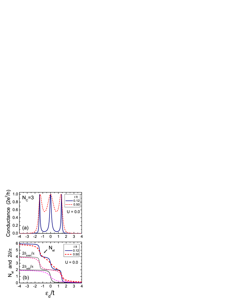
Figure 5: The conductance $g_{\rm series}$, and total charge in the triple-dot $N_{\rm el}$ in the noninteracting case $U=0$ as functions of $\epsilon_{d}/t$ for (solid line) $\Gamma/t=0.12$ and (dashed line) $\Gamma/t=0.5$. The phase shifts $2\delta_{\rm even}/\pi$ and $2\delta_{\rm odd}/\pi$ are also shown in (b).

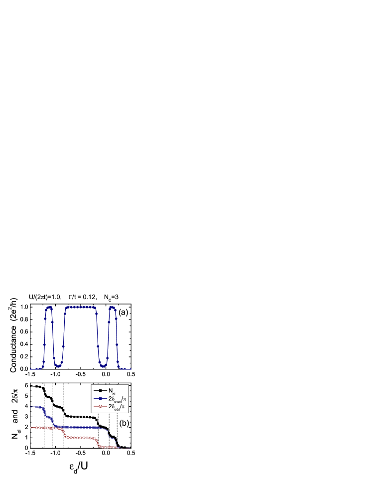
Figure 6: The conductance $g_{\rm series}^{\phantom{0}}$, local charge $N_{\rm el}$, phase shifts $2\delta_{\rm even}/\pi$ and $2\delta_{\rm odd}/\pi$ for the triple dot as a function of $\epsilon_{d}/U$ for $U/(2\pi t)=1.0$ and $\Gamma/t=0.12$. The dashed vertical lines in (b) show the values of $\epsilon_{d}$ at which $N_{\rm el}$ jumps in the “molecule limit” $\Gamma=0$. For NRG, we use $t/D=0.1$ and $\Lambda=6.0$.

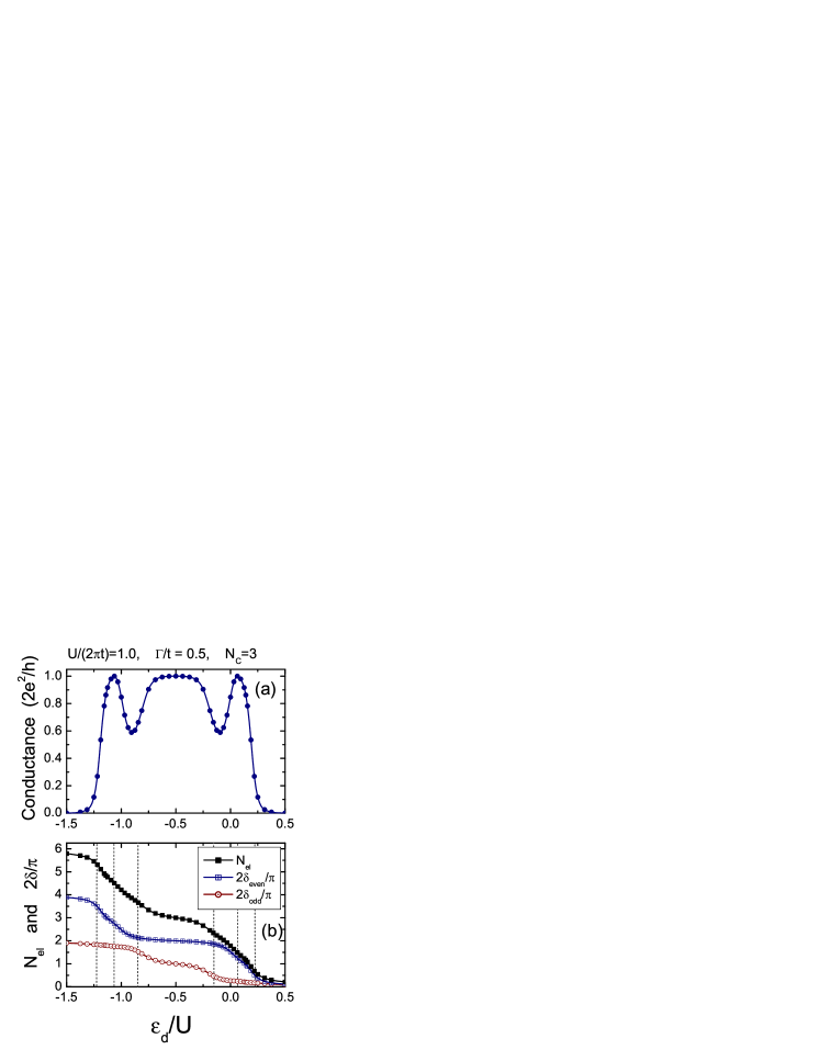
Figure 7: The conductance $g_{\rm series}^{\phantom{0}}$, local charge $N_{\rm el}$, phase shifts $2\delta_{\rm even}/\pi$ and $2\delta_{\rm odd}/\pi$ for the triple dot as a function of $\epsilon_{d}/U$ for $U/(2\pi t)=1.0$ and $\Gamma/t=0.5$. The dashed vertical lines in (b) show the values of $\epsilon_{d}$ at which $N_{\rm el}$ jumps in the limit of $\Gamma=0$. For NRG, we use $t/D=0.02$ and $\Lambda=6.0$.

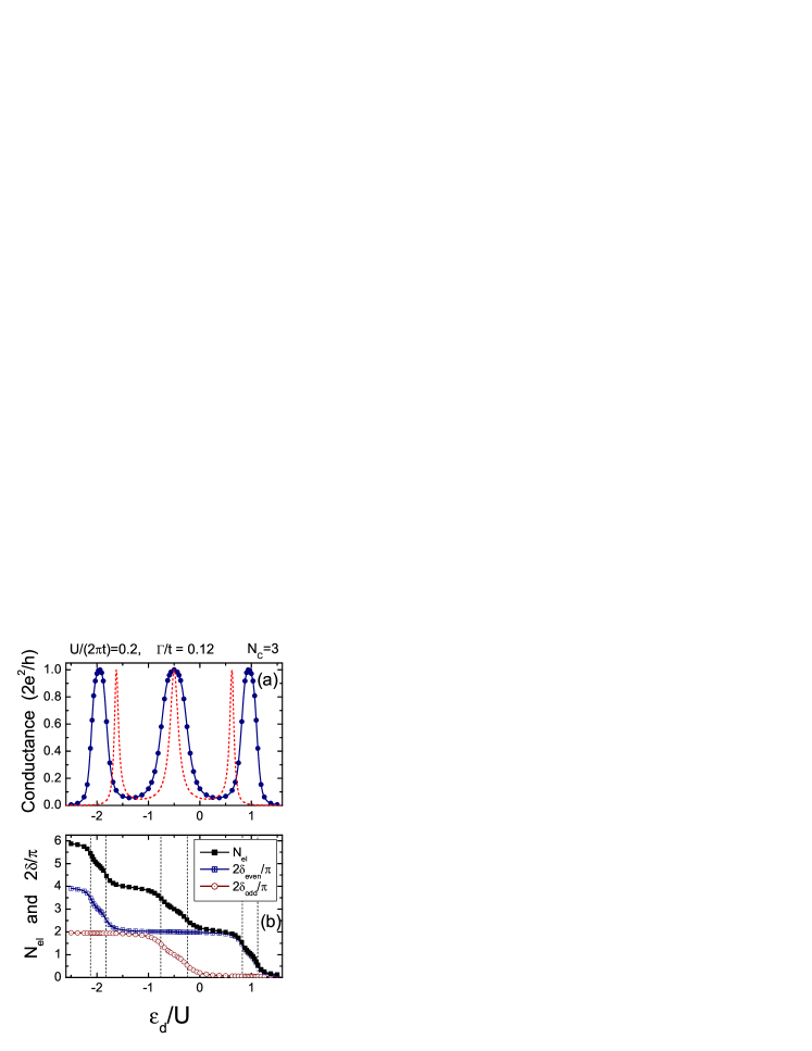
Figure 8: The conductance $g_{\rm series}^{\phantom{0}}$, local charge $N_{\rm el}$, phase shifts $2\delta_{\rm even}/\pi$ and $2\delta_{\rm odd}/\pi$ for the triple dot as a function of $\epsilon_{d}/U$ for $U/(2\pi t)=0.2$ and $\Gamma/t=0.12$. In (a) the dashed line corresponds to the results for $U=0$: it is shifted to the negative energy region by $-U/2$ so that the position of the central peak coincides with that of the interacting case, and also the energy is scaled by $U$ using $U/(2\pi t)=0.2$. The dashed vertical lines in (b) show the values of $\epsilon_{d}$ at which $N_{\rm el}$ jumps in the limit of $\Gamma=0$. For NRG, we use $t/D=0.1$ and $\Lambda=6.0$.

4.1 Series connection

We first of all discuss the noninteracting case $U=0$. In Fig. 5, the conductance $g_{\rm series}$, local charge in the triple dot $N_{\rm el}$, and the phase shifts are plotted as functions of $\epsilon_{d}/t$ for (solid line) $\Gamma/t=0.12$ and (dashed line) $\Gamma/t=0.5$. The conductance shows sharp peaks when the resonance states in the triple dot cross the Fermi level. Among the three conductance peaks, the one in the middle corresponds to an orbitals with the odd parity, and the remaining two belong to the orbitals with the even parity. For $U=0$, the two phase shifts are given by $\cot\delta_{\rm even}=\left(\epsilon_{d}^{2}-2t^{2}\right)/\left(\Gamma\epsilon_{d}\right)$, and $\cot\delta_{\rm odd}=\epsilon_{d}/\Gamma$. The phase shifts show a step of the height $\pi$, when the resonance state of the corresponding parity crosses the Fermi level. Simultaneously, the local charge $N_{\rm el}$ also shows a staircase behavior, and the step corresponding to two electrons, spin up and spin down, occupying the resonance states. For large $\Gamma$, the resonance peaks become broad, and the steps in the phase shifts vanish gradually.

For interacting case $U\neq 0$, we have carried out the NRG iterations by introducing the bonding and anti-bonding orbitals also for the leads; $(f^{\dagger}_{n,R\sigma}\pm f^{\dagger}_{n,L\sigma})/\sqrt{2}$. In the present study, instead of adding these two orbitals at $n=N+1$ simultaneously for constructing the Hilbert space for the next NRG step, we add the bonding orbitals first and retain typically 3600 low-energy states after carrying out the diagonalization. Then, we add the remaining anti-boding orbitals, and carry out the truncation again keeping the lowest 3600 eigenstates. This truncation procedure preserves the inversion symmetry, and in the case of odd $N_{C}$ it also preserves the particle-hole symmetry at $\epsilon_{d}=-U/2$. With this procedure, the discretized Hamiltonian $H_{N}$ can be diagonalized exactly up to $N=1$, where the total number of the sites in the cluster is $N_{C}+2(N+1)=7$ for the triple dot $N_{C}=3$ as illustrated in Fig. 3. For $N\geq 2$, we have confirmed that the eigenvalues in the noninteracting limit $U\to 0$ are reproduced sufficiently well with this procedure for the discretization parameter of the value $\Lambda=6.0$.

We have also confirmed that the fixed-point eigenvalues of the NRG for the triple dot can be described by the quasi-particle Hamiltonian defined in eq. (39) for all parameter values we have examined. It justifies the assumption of the local Fermi liquid we have made to derive eq. (38). In Fig. 6, the NRG results for (a) the conductance $g_{\rm series}^{\phantom{0}}$, (b) phase shifts $\delta_{\rm even}$, $\delta_{\rm odd}$ and total charge in the triple dot $N_{\rm el}$ are plotted as a function of $\epsilon_{d}/U$ for $U/(2\pi t)=1.0$. Here the hybridization is relatively small $\Gamma/t=0.12$ compared to the hopping matrix element $t$, which is taken to be $t/D=0.1$ in the NRG iterations. The vertical dotted lines in (b) correspond to the values of $\epsilon_{d}$ at which $N_{\rm el}$ jumps discontinuously in a ‘molecule’ limit $\Gamma\to 0$. The local charge $N_{\rm el}$ shows a step behavior near the dotted lines. Specifically, due to the Coulomb interaction, the steps emerge also for odd $N_{\rm el}$. These odd steps reflect the $\pi/2$ steps of the phase shifts. The conductance shows the typical Kondo plateaus of the Unitary limit $g\simeq 2e^{2}/h$ in the regions of $\epsilon_{d}$ corresponding to the odd occupancies $N_{\rm el}\simeq 1$, $3$, $5$. In contrast, the conductance shows wide minima for even occupancies $N_{\rm el}\simeq 2$, $4$. These features are linked to the behavior of the phase shifts; $\delta_{\rm even}-\delta_{\rm odd}\simeq\pi/2$ for odd $N_{\rm el}$, and $\delta_{\rm even}-\delta_{\rm odd}\simeq 0$ or $\pi$ for even $N_{\rm el}$.[16]

Among the three conductance plateaus, the one in the middle is wider than the others. This seems to be caused by the suppression of the charge fluctuation near half-filling. It is expected that the plateau becomes wider for some particular values of $N_{\rm el}$, at which the charging energy defined with respect to the unconnected limit $\Gamma=0$ is large. Thus, a wide plateau may emerge for the filling near the metal-insulator transition, which generally depends on the spatial range of the repulsive interaction.

We next consider the case where the triple dot is coupled strongly to the leads via a large hybridization. In Fig. 7, the NRG results obtained at $\Gamma/t=0.5$ are shown, where the value of the Coulomb interaction is unchanged $U/(2\pi t)=1.0$. The local charge $N_{\rm el}$, which shows a staircase behavior for small $\Gamma$ in Fig. 6, becomes now a gentle slope in Fig. 7 (b) due to the large hybridization. Correspondingly, the shoulders of the conductance plateaus become round, and the valleys become shallow. Nevertheless, near half-filling, the phase shift for the odd partial wave still shows a weak $\pi/2$ step, i.e., $\delta_{\rm odd}\simeq\pi/2$ near half-filling. It keeps the conductance peak at the center flat. Note that in this calculation the hopping matrix element is taken to be $t/D=0.02$, but the change in this ratio does not affects the low-energy properties so much.

We also examine the case with a weak interaction $U/(2\pi t)=0.2$ and small hybridization $\Gamma/t=0.12$. The results are shown in Fig. 8. It shows an early stage of a development of the Kondo plateaus. In the upper panel (a), the dashed line corresponds to the conductance in the noninteracting case: for comparison it is shifted to the negative energy region by $-U/2$ so that the positions of the central peak coincides with that for the interacting case, and also the energy is scaled by $U$ using the value $U/(2\pi t)=0.2$. Due to the Coulomb interaction, the conductance peaks become wider than that for the noninteracting electrons, and the form of the peaks deviates from the simple Lorentzian shape. Furthermore, the separation of the peaks increases. Since $U$ is not so large in this case, the local charge $N_{\rm el}$ becomes flat only for even occupancies $N_{\rm el}=0,2,4,6$. It reflects the behavior of the phase shifts, i.e., both $\delta_{\rm even}$ and $\delta_{\rm odd}$ do not show the clear $\pi/2$ steps. Nevertheless, the slopes in between the $\pi$ steps become longer compared to the ones in the noninteracting case, and weak precursors for the development of the $\pi/2$ steps can be seen in these slopes.

4.2 Parallel conductance

The parallel conductance through the tripled dot as illustrated in Fig. 9, can be evaluated via eq. (29) with the phase shifts for the series connection given in the above. This is because, as mentioned in §2, the matrix Green’s function $\mbox{\boldmath$G$}(z)$ for the interacting sites for the parallel connection coincides with that for the series connection owing to the inversion symmetry for the leads in the horizontal direction, as described in Fig. 2. Thus a site-diagonal quantity such as local charge $N_{\rm el}$ becomes the same with that for the series connection as mentioned in §2. The conductances, however, are different. It opens a way to determine the values the phase shifts $\delta_{\rm even}$ and $\delta_{\rm odd}$ from measurements of the series and parallel conductances using eqs.  (27) and (29).

Figure 9: Schematic picture of a parallel connection for $N_{C}=3$.

We first of all consider the noninteracting case. In Fig. 10, the parallel (solid line) and series (dashed line) conductances for $U=0$ are plotted as functions of $\epsilon/t$ for (a) $\Gamma/t=0.12$ and (b) $\Gamma/t=0.5$. In (a), the two curves almost overlap each other, and the difference between the parallel and series conductances can be seen only near the two valleys corresponding to even $N_{\rm el}$. The both conductances show a similar feature due to the three resonance states. At half-filling, $\epsilon_{d}=0$ for noninteracting electrons, the two curves contact with each other. This is because the phase shifts take the values $\delta_{\rm even}=\pi$ and $\delta_{\rm odd}=\pi/2$. The phase shifts do not show such an exact synchronism at the side resonance peaks corresponding to $N_{\rm el}\simeq 1$ and $5$, and there the parallel conductance become larger than $2e^{2}/h$, which is possible because two conducting channels contribute to the current in the parallel connection. The parallel conductance becomes larger than the series conductance for $|\epsilon_{d}|\gtrsim 2t$. This is because the both phase shifts show the same asymptotic behavior, $\delta_{\rm even}\simeq\Gamma/\epsilon_{d}$ and $\delta_{\rm odd}\simeq\Gamma/\epsilon_{d}$, for $\epsilon_{d}\to\infty$, and a similar cancellation occurs for the series conductance also in the opposite limit $\epsilon_{d}\to-\infty$. The difference between the parallel and series conductances becomes small for small $\Gamma$.

In Fig. 11, the (solid circle) parallel and (open square) series conductances in the interacting case $U/(2\pi t)=1.0$ are plotted as a function of $\epsilon_{d}/U$ for (a) $\Gamma/t=0.12$ and (b) $\Gamma/t=0.5$. The difference between $g_{\rm parallel}$ and $g_{\rm series}$ for interacting electrons is similar, qualitatively, to that in the noninteracting case, although the appearance of the Kondo plateaus changes the overall feature of the $\epsilon_{d}$ dependence. In (a) the difference are visible only near the conductance valleys. For large $\Gamma$, however, the difference becomes larger, and it can be seen whole region plotted in (b) except near the central plateau. As in the noninteracting case, the parallel conductance becomes larger than $2e^{2}/h$ at the side Kondo plateaus corresponding to $N_{\rm el}\simeq 1$ and $3$ due to the contributions of the two conducting modes. The conductance valleys corresponding to even $N_{\rm el}$ become deeper for the parallel conductance than that of the series conductance. However, the difference is small for small $\Gamma$.

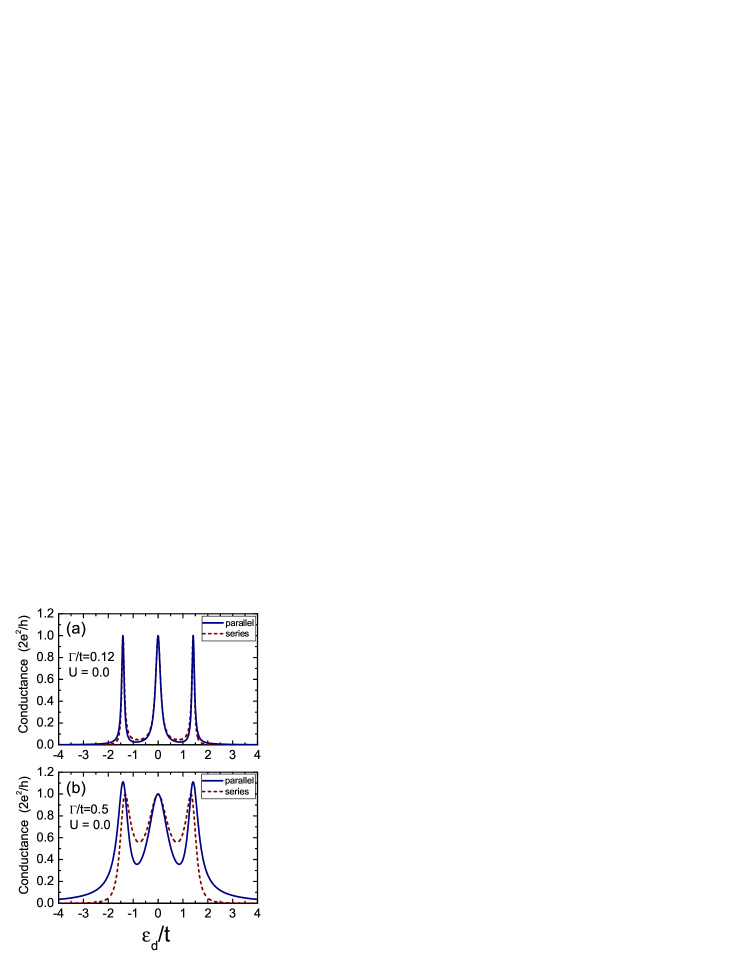
Figure 10: The conductance in the parallel (solid line) and series (dashed line) connections for noninteracting electrons $U=0$ as functions of $\epsilon_{d}/t$, where (a) $\Gamma/t=0.12$ and (b) $\Gamma/t=0.5$. Note that two conducting channels contribute to the parallel conductance, so that the upper bound for $g_{\rm parallel}$ is not $2e^{2}/h$.

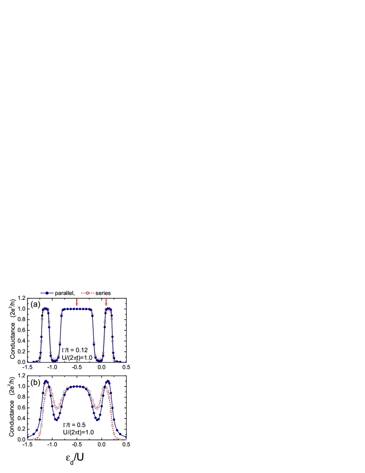
Figure 11: The conductance in the parallel (solid line) and series (dashed line) connections for interacting electrons $U/(2\pi t)=1.0$ as functions of $\epsilon_{d}/U$, where (a) $\Gamma/t=0.12$ and (b) $\Gamma/t=0.5$. The two arrows in (a) indicate the points, for which the energy flow is described in Fig. 12.

5 Discussion

The results presented in the above have been obtained at zero temperature. Nevertheless the Kondo behavior we have discussed can be seen at low enough temperatures $T\lesssim T_{K}$, although the height of the Kondo plateaus will decrease gradually with increasing $T$ from the Unitary-limit value as that in the single impurity case.[12] At $T\gg T_{K}$, the plateaus finally disappear and the conductance shows the oscillatory behavior of the Coulomb blockade with the peaks, the height of which is about half of the Unitary-limit value.[16] The Kondo temperature $T_{K}$ decreases with increasing $U$, and a large number of the NRG iteration $N$ is required to get to the Fermi-liquid fixed point that determines the low-energy Kondo behavior for large $U$.[13] The value of $T_{K}$ should be different for different plateaus. Specifically, for the central plateaus near half-filling, $T_{K}$ becomes small for the Hubbard chain with large size $N_{C}$ because the developing Mott-Hubbard (pseudo) gap disturbs the screening of the local moment.

In order to estimate the Kondo energy scale for different plateaus, the flow of the low-lying eigenvalues of $H_{N}/D$ for the triple-dot is plotted in Fig. 12 as a function of odd $N$ for $U/(2\pi t)=1.0$ and $\Gamma/t=0.12$. This parameter set is the same as the one used for Fig. 6 and Fig. 11 (a). The figure 12 (a) shows the flow at the central Kondo plateau for $\epsilon_{d}/U=-0.5$, and the lower panel (b) shows the flow at the right plateau for $\epsilon_{d}/U\simeq 0.15625$. The positions corresponding to these two values of $\epsilon_{d}$ are indicated in Fig. 11 (a) by the arrows. In the figure 12, the crossover from the high-energy region to low-energy Fermi-liquid regime can be seen clearly. For large $N$, the energy levels converge to the fixed-point values, and the many-body eigenvalues of $H_{N}/D$ have one-to-one correspondence with the free quasi-particle excitations.[13, 9, 10] The number of NRG iterations $N^{*}$ needed to reach the low-energy regime in each of the plateaus is estimated to be (a) $N^{*}\simeq 30$, (b) $N^{*}\simeq 15$, and $N^{*}\simeq 15$ also for the left plateau, for which the energy flow is identical to Fig. 12 (b) except for the values of some quantum numbers assigned to the lines. The crossover occurs at an energy $T^{*}\simeq D\Lambda^{-(N^{*}-1)/2}$, where a factor of the form $\Lambda^{-(N-1)/2}$ emerges to recover the energy scale of the original Hamiltonian ${\cal H}$ from the discretized version $H_{N}$ defined in eq. (30). The crossover energy reflects the width of the Kondo resonance, so that $T^{*}\sim T_{K}$ apart form a numerical factor of order O(1) which depends on the precise definition of $T_{K}$. Consequently, these results show that the Kondo energy scale for the central plateau at half-filling is much smaller than that for the side plateaus away from half-filling.

In order to calculate the conductance for whole temperature ranges, one generally has to use several different approaches. The behavior at high temperatures $T>T_{K}$ can be captured, for instance, by the exact diagonalization of small clusters, such as the one examined by several authors.[24, 25] At low temperatures, however, one needs the information about the low-energy excitations. From the Fermi-liquid regime to the crossover region near $T_{K}$, the conductance can be calculated from the current-current correlation function using NRG method.[11, 12] The ground-state value of the conductance can be calculated from the phase shifts, which can be deduced efficiently from the low-energy eigenvalues using eq. (38).

In summary, we have described the method to deduce the phase shifts for finite interacting systems attached to noninteracting leads from the fixed point Hamiltonian of NRG. Our approach assumes the inversion symmetry, but does not assume a specific form of the Hamiltonian nor electron-hole symmetry, and thus it is applicable to a wide class of quantum impurities. We apply the method to a triple quantum dot of $N_{C}=3$ connected to two noninteracting leads, and calculate the dc conductance away from half-filling as a function of the onsite energy $\epsilon_{d}$. At $T=0$, the conductance shows the Kondo plateaus of the Unitary limit $g\simeq 2e^{2}/h$ at the values of gate voltage corresponding to odd numbers of electrons $N_{\rm el}$, while it shows the wide minima for even $N_{\rm el}$. It seems to be natural to expect that these low-temperature properties seen at $T\lesssim T_{K}$ are common to the Hubbard chain of finite size $N_{C}$ attached to Fermi-liquid reservoirs.

Figure 12: Low energy levels of $H_{N}/D$ are plotted as a function of odd $N$ for (a) $\epsilon_{d}/U=-0.5$ where $N_{\rm el}=3$, and (b) $\epsilon_{d}/U=0.15625$ where $N_{\rm el}\simeq 1$. Other parameters are the same with those in the case of Fig. 6: $U/(2\pi t)=1.0$ $\Gamma/t=0.12$, $t/D=0.1$ and $\Lambda=6.0$. The label ($Q$, $2S$, $p$) corresponds to the charge $Q$, spin $S$, and parity $p$ ($=$ even, or odd).

References

- [1] L. I. Glazman and M. E. Raikh: JETP Lett. 47 (1988) 452.
- [2] T. K. Ng and P. A. Lee: Phys. Rev. Lett. 61 (1988) 1768.
- [3] D. Goldharber-Gordon, H. Shtrikman, D. Mahalu, D. Abusch-Magder, U. Meirav, and M. A. Kastner: Nature 391 (1998) 156.
- [4] S. M. Cronenwett, T. H. Oosterkamp, and L. P. Kouwenhoven: Science 281 (1998) 540.
- [5] W. Hofstetter, J. König, and H. Schoeller: Phys. Rev. Lett. 87 (2001) 156803.
- [6] K. Kobayashi, H. Aikawa, S. Katsumoto, and Y. Iye: Phys. Rev. Lett. 88 (2002) 256806.
- [7] A. Oguri, Y. Tanaka, and A. C. Hewson: J. Phys. Soc. Jpn. 73 (2004) 2494.
- [8] K. G. Wilson: Rev. Mod. Phys. 47 (1975) 773.
- [9] H. R. Krishna-murthy, J. W. Wilkins: and K. G. Wilson, Phys. Rev. B 21 (1980) 1003.
- [10] H. R. Krishna-murthy, J. W. Wilkins: and K. G. Wilson, Phys. Rev. B 21 (1980) 1044.
- [11] W. Izumida, O. Sakai, and Y. Shimizu: J. Phys. Soc. Jpn. 67 (1998) 2444.
- [12] W. Izumida and O. Sakai: Phys. Rev. B 62 (2000) 10260; J. Phys. Soc. Jpn. 74 (2005) 103.
- [13] A. Oguri and A. C. Hewson: J. Phys. Soc. Jpn. 74 (2005) 988.
- [14] A. C. Hewson, A. Oguri, and D. Meyer: Eur. Phys. J. B 40 (2004) 177.
- [15] A. C. Hewson: J. Phys. Soc. Jpn. 74 (2005) 8.
- [16] A. Kawabata, J. Phys. Soc. Jpn. 60, 3222 (1991).
- [17] A. Oguri: Phys. Rev. B 59 (1999) 12240.
- [18] A. Oguri: Phys. Rev. B 63 (2001) 115305; ibid. [Errata: 63 (2001) 249901].
- [19] A. Oguri: J. Phys. Soc. Jpn. 70 (2001) 2666; ibid. 72, 3301 (2003).
- [20] J. S. Langer and V. Ambegaokar, Phys. Rev. 121 (1961) 1090.
- [21] Y. Tanaka, A. Oguri, and H. Ishii: J. Phys. Soc. Jpn. 71 (2002) 211.
- [22] A. C. Hewson: J. Phys.: Condens. Matter 13 (2001) 10011.
- [23] O. Sakai, Y. Shimizu, and T. Kasuya: Prog. Theor. Phys. Suppl. 108 (1992) 73.
- [24] G. Chiappe and J. A. Vergés: J. Phys.: Condens. Matter 15 (2003) 8805.
- [25] C. A. Büsser, A. Moreo, and E. Dagotto: Phys. Rev. B 70 (2004) 035402.