Contact and Quasi-Static Impact of a Dissipationless Mechanical Model

Abstract

Collisions and contacts of elastic materials are numerically and theoretically investigated. Using a two-dimensional spring-mass model with defect particles under the free boundary condition, we reproduce the Hertzian contact theory at equilibrium and the quasi-static theory for low speed impacts.

1 INTRODUCTION

The origin of irreversibility from a reversible mechanical model is one of the most fundamental subjects in non-equilibrium statistical mechanics. A typical example can be seen in transport phenomena in nonlinear spring models[1, 2]. Although most of models discuss the transport processes under the influence of thermostats, we still do not understand the mechanism to reach an equilibrium state based on a purely mechanical model.

The aim of this paper is to derive macroscopic laws of elastic materials based on a microscopic lattice model. Here we discuss contacts and impacts between elastic materials. The former is related to the origin of the second law of thermodynamics from a purely mechanical model.

For contacts of elastic materials, we believe that the contacts between elastic bodies can be described by the Hertzian contact theory[3, 4, 5]. The two-dimensional Hertzian contact theory gives us the relation between the deformation of a disk $\delta$ and the compressive force $P$ as

$$\delta\simeq\frac{P}{\pi E^{*}}\left\{\ln\left(\frac{4\pi E^{*}R}{P}\right)-1-\nu\right\},$$ (1)

where $R$ is the radius of the undeformed disk[6]. Here, $E^{*}$ is the reduced Young’s modulus, $E^{*}=E/(1-\nu^{2})$, where $E$ and $\nu$ are Young’s modulus and Poisson’s ratio, respectively.

For the low speed head-on collisions of elastic materials, the relation between the restitution coefficient $e$ and the impact speed $v$ is described by the quasi-static theory of low speed impacts[7, 8]. The quasi-static theory is an extension of the Hertzian contact theory to include the internal viscosity of materials. By solving the equation of motion for the deformation with adequate initial conditions and calculating the rebound speed, we can obtain the relation between the impact speed $v$ and the restitution coefficient $e$.

The restitution coefficient $e$ depends also on the incident angle[9, 10]. We have recently carried out a two-dimensional simulation of oblique impacts using a dissipationless elastic model based on the mass-spring model [11, 12] to reproduce and explain the previous experimental result by Louge and Adams[9]. Although the model can reproduce similar results to the experimental results, one of the apparent defects in the model is that the system cannot reach an equilibrium state described by the Hertzian contact theory[3, 4, 5]. When we put the disk on the wall under the influence of the gravity, the release of initial potential energy is recurrent and the system keeps oscillations. We also have expected that $e$ can be described by the quasi-static theory for low speed head-on collision of the disk with a potential wall, but we have found a discrepancy between the numerical result and the prediction by the quasi-static theory[6, 13]. Refining the model to overcome those defects in a dissipationless model will be helpful to understanding the origin of irreversibility and the second law of thermodynamics from a mechanical point of view.

In this paper, we propose a microscopic dissipationless model to reproduce the Hertzian contact at equilibrium and the quasi-static theory for low-speed impacts. These results enable us to understand the origin of irreversibility for finite degrees of freedom from a reversible mechanical model. The construction of this paper is as follows. In the next section we introduce our model. In Sec. 3 and 4 we show the results of our simulation of contact problems and low-speed impacts, respectively, and briefly summarize our results. Appendix A is devoted to the calculation of elastic moduli of our model.

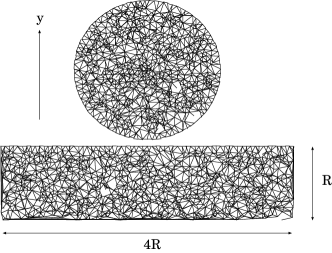
Figure 1: The elastic disk and wall consisted of random lattice. We set $y=0$ at the surface of the wall. In this figure, the height and the width of the wall are respectively $R$ and $4R$ with the undeformed radius of the disk $R$.

2 Model

Let us introduce our model(Fig.1). It is basically the same as our previous model which obeys Hamilton equation[14, 11]. The disk consists of $1099$ mass points while the wall consists of $1269$ mass points. The two corner points of the bottom of the wall are fixed. The surfaces of both the disk and the wall are initially flat. The interaction between the disk and the wall is introduced as follows. Each mass point $i$ on the lower half boundary of the disk receives the force, ${\bf F}(l_{s}^{(i)})=aV_{0}\exp(-al_{s}^{(i)}){\bf n}_{s}^{(i)}$, where $l_{s}^{(i)}$ is the distance between $i$-th surface mass point of the disk and the nearest surface spring of the wall, $a=500/R$, $V_{0}=amc^{2}R/2$, $m$ is the mass of each mass point $i$, $c$ is the one-dimensional speed of sound, and ${\bf n}_{s}^{(i)}$ is the unit vector normal to the connection between two surface mass points of the wall[14, 11]. Thus, the dynamical equation of motion for each mass point $i$ of the lower half boundary of the disk is described by

$$m\frac{d^{2}{\bf r}_{i}}{dt^{2}}=\sum^{N_{i}}_{j=1}\left\{-k_{a}{\bf x}_{ij}-k_{b}{\bf x}_{ij}^{3}\right\}+\Theta(l_{th}-l_{s}^{(i)})aV_{0}\exp(-al_{s}^{(i)}){\bf n}_{s}^{(i)},$$ (2)

where ${\bf r}_{i}$ is the position of $i$-th mass point, $t$ is the time, $N_{i}$ is the number of mass points connected to $i$-th mass point, ${\bf x}_{ij}$ is the relative deformation vector of the spring from the natural length between $i$-th and $j$-th connected mass points, $k_{a}$ and $k_{b}=k_{a}\times 10^{-3}/R^{2}$ are the spring constants. Here $\Theta(x)$ is the step function, i.e. $\Theta(x)=1$ for $x\geq 0$ and $\Theta(x)=0$ for $x<0$, and the threshold length $l_{th}$ is the average of the natural lengths of the springs of the disk. For internal mass points, the last term of the right hand side of eq.(2) is omitted. In most of our simulations, we adopt $k_{a}=k^{(d)}_{a}=1.0\times mc^{2}/R^{2}$ for the disk and $k_{a}=k^{(w)}_{a}=1.0\times 10^{2}mc^{2}/R^{2}$ for the wall. Numerical integration of eq.(2) is performed by the fourth order symplectic integrator with the time step $dt=10^{-3}R/c$.

There are two main differences between our new model and the previous model. Here we introduce some defect particles and adopt the free boundary condition in which the kinetic energy can escape from the boundary. The defect particles are introduced by choosing mass point $i$ at random and eliminating $N_{i}-1$ connecting bonds among $N_{i}$ connecting bonds to $i$-th mass point. We have introduced $10$ defects for each body. The reason to choose $10$ defects will be discussed later. With the introduction of these defects, we expect that the motion of defects becomes irregular and the vibrating wave can be localized without spreading. This irregular motion may create the irreversibility of time evolution of mass points. In addition, we adopt the free boundary condition for both sides and the bottom of the wall in contrast to the reflective boundary condition in our previous model. We regard the wall as a part of a large system. When we put a mechanical perturbation in the wall such as a contact or an impact, the effect propagates as elastic waves and goes out from the boundary because our system is a part of a larger system. In this situation, ${\bf J}\cdot{\bf n}_{b}>0$ should be satisfied where ${\bf n}_{b}$ and ${\bf J}$ are respectively the unit normal vector on the boundary and the energy flux ${\bf J}=\sum_{i}\{(1/2)m{\bf v}_{i}^{2}+\epsilon_{i}\}{\bf v}_{i}$ with the potential energy $\epsilon_{i}$. In order to realize the condition, at each time step of numerical integration, we set ${\bf v}_{i}={\bf 0}$ if ${\bf v}_{i}$ is directed to inner region of the wall. Because the reflected wave does not come into the system, the total energy of our system is not conserved.

Here we briefly comment on the boundary condition we adopt. Our model does not conserve the total energy because there is the outgoing energy flux from the system. We can put thermostats, e.g. Nosé-Hoover thermostats[15], on the boundary to keep the energy conservation law. However, once we introduce the thermostat in the system, the phase volume is not conserved, and there is the entropy production[16]. In addition, we believe that the thermalization from the thermostat does not play an important role in macroscopic elastic materials[13]. Thus, we adopt the model without the conservation of the energy. In the next section we will show that the introduction of the thermostat does not make much difference in our results.

3 Simulation of Contact Problems

In this section, we show the results of our simulation of elastic contacts. At first, we show the results of the simulation for the contact problem.

Figure 2: The relation between the deformation and the external force. Cross points with error bars are the numerical results with the initial temperature $T=0$. Plus points are the numerical results with the initial temperature $T=10^{-7}Mc^{2}$ in the simulation with Nosé-Hoover thermostats. The solid line is the prediction by the Hertzian contact theory with $\nu=0.336$.

In this simulation, we introduce the wall whose height and width are $4R$ and $R$, respectively. We put the disk in the external field $P$ ranging from $P=5.77\times 10^{-3}\pi RE^{*}$ to $P=1.27\times 10^{-2}\pi RE^{*}$. Thus, in this case, we add the term $-(P/N){\hat{\bf y}}$ in the right hand side of eq.(2), where $N=1099$ and ${\hat{\bf y}}$ is the unit vector in $y$ direction. The initial oscillation of the center of mass of the disk relaxes to reach a stable oscillation. After the relaxation of the center of mass, we calculate the deformation of the disk, $\delta\equiv R-R_{d}$, where $R_{d}$ is the deformed radius of the disk which is the distance from the contact patch to the center of mass of the disk.

Figure 2 is the relation between $\delta/R$ and $P/\pi RE^{*}$. Cross points are the averaged results of $10$ disks with different configuration of mass points, and the error bars are the standard deviations. The solid line in Fig.2 is eq.(1) with $\nu=0.336$ calculated from the two-dimensional theory of elasticity based on the assumption of an isotropic disk. Details of the calculation of elastic constants of the model are shown in Appendix AA. Our simulation data are well reproduced by the theoretical curve which does not include any fitting parameters. Thus, we conclude that our model can produce an equilibrium state at the contact.

Let us discuss the effect of thermalization from thermostats on our results. We have carried out another simulation, in which the wall has fixed boundaries at the bottom and the both side ends, and the mass points connected to the fixed boundaries obey the equation of motion of particles connected to the Nosé-Hoover thermostat[15]. We have arranged that the temperature of the wall becomes $T=10^{-7}Mc^{2}$. Here we define the temperature of the thermostat by the variance of the Maxwell-Boltzmann distribution which we give as the initial velocity distribution of the thermostat particles. Plus points in Fig. 2 are the averaged results of $10$ disks with different configuration of mass points in the simulation with the Nosé-Hoover thermostat. This result shows that the introduction of thermostats does not affect the relation between the compressive force and the deformation so much. From this result, we conclude that the thermlization from the thermostat does not play an important role in our simulation of contact problems.

Introducing defect particles in the model plays an important role in the relaxation of internal vibration in the contact problem. To characterize the relaxation process to an equilibrium state, we investigated the time evolution of the velocity distribution function (VDF) $f(v_{x},v_{y},t)$, where $v_{x}$ and $v_{y}$ are velocity components of mass points of the disk, and the Shannon entropy when the compressive force $P=8.75\times 10^{-3}\pi RE^{*}$. To obtain the velocity distribution function $f(v_{x},v_{y},t)\equiv\sum_{x}\sum_{y}f(x,y,v_{x},v_{y},t)$, we calculate $f(x,y,v_{x},v_{y},t)$ by averaging the data from $t-6R/c$ to $t$.

Figure 3: The velocity distribution of mass points of the disk at (a) $t=t_{0}$ and (b) $t=t_{max}$.

Figure 4: The time evolutions of the Shannon entropy $S(t)$ when the number of defects are (a) from 8 to 10 and (b) 0 and 15. X-axis is the scaled time while y-axis is the Shannon entropy $S(t)$ calculated from the distribution function of internal mass points of the disk.

Figure 3 shows the time evolution of VDF $f(v_{x},v_{y},t)$. The distribution function near the initial stage (Fig. 3(a)), $f(v_{x},v_{y},t_{0}=6R/c)$, has three peaks along the axis $v_{x}=0$. The peaks may be attributed to the coexistence of the reflective motion and the compressive motion of mass points in the disk. Figure 3(b) shows that $f(v_{x},v_{y},t_{max}=60R/c)$ has a Gaussian form. In fact, $f(v_{x},0,t_{max})$ can be well fitted by the Gaussian whose variance is $0.02$.

In addition, we have investigated the time evolution of the Shannon entropy. Figure 4 shows the time evolution of the entropy defined by $S(t)\equiv-\sum_{x}\sum_{y}\sum_{v_{x}}\sum_{v_{y}}f(x,y,v_{x},v_{y},t)\ln f(x,y,v_{x},v_{y},t)$ for several numbers of defects. We have investigated the dependence of the number of defect particles on the entropy. In Fig.4, we change the number of defects in the disk from $0$ to $15$, and investigate the time evolution of the entropy for each disk. In the case of the disks whose number of defects are from $8$ to $10$, after $t=30R/c$, the time evolution of the entropy is described as an universal curve which shows monotonic increase and reaches the maximum value $13.5$. In the case of other disks, the entropy does not show the monotonic increase. The mixing effect is not enough for the smaller number of defects while a global oscillation is excited because of the weakness of the disk structure for too large number of defects.

We have also calculated the averaged kinetic energy per one defect particle (Fig.5). The time averaged kinetic energy of one defect is not so large as that of the other particles. However, the kinetic energy for one defect changes at random with larger amplitude. This tendency originates from irregular motion of the defect particles, which enables the oscillation modes to mix and to reach an equilibrium state. In realistic systems, such a phenomenon can be seen in phonon scattering by defects and impurities of solids, the scattering which realizes a thermal equilibrium state. We conclude that the irregular motion of the defect particles generates irreversibility and makes the model reach an equilibrium state, which reproduces the Hertzian contact of our model.

Figure 5: The time evolution of the kinetic energy per one particle of bound particles and defect particles of the disk.

4 Simulation of Low-speed Impact

In this section, we show the results of the simulation of low speed impact. Here we arrange that the height and the width of the wall are respectively $R$ and $4R$. From the simulation of the head-on collision of the disk with the wall, we calculate $e$ for each initial speed. The initial speed is ranged from $v=1.0\times 10^{-3}c$ to $v=1.0\times 10^{-2}c$ without the external field.

Figure 6: The relation between the colliding speed $v$ and the restitution coefficient $e$. The solid line indicates the prediction by the quasi-static theory. The cross points with error bars are numerical results in the range (a) from $v/c=0.001$ to $v/c=0.02$ and (b) from $v/c=0.001$ to $v/c=0.007$.

Figure 6 (a) is the relation between the restitution coefficient $e$ and the impact speed $v/c$ ranging from $v/c=0.001$ to $v/c=0.02$ while Fig. 6 (b) is the results in the low colliding speed. The cross points are the averaged results of $10$ disks with different configuration of mass points, and the error bars are the standard deviations. As can be seen, $e$ decreases slightly with increasing colliding velocity and $e$ cannot reach $1$ as impact velocity decreases. We compare this result with the two-dimensional quasi-static theory of low speed impact[8, 7, 17]. In the two-dimensional quasi-static theory[18], the dynamical equation of motion for the deformation of the disk may be written as

$$M\frac{d^{2}\delta}{dt^{2}}=-P-\tau_{0}\frac{dP}{d\delta}\frac{d\delta}{dt},$$ (3)

where $M$ is the mass of the disk and $\tau_{0}$ is the time scale of dissipation. $P$ is obtained as a function of $\delta$ by numerically solving eq.(1) for $P$. The last term in the right hand side is the dissipative force which is proportional to the velocity of the deformation[8, 7]. By introducing $\tau_{0}$ as a fitting parameter, we solve eqs.(1) and (3) numerically with the initial conditions $\delta=0$ and $d\delta/dt=v$ to obtain the relation between $e$ and $v$. The solid line in Fig. 6 (a) and (b) is the numerical result of eq.(3) with $\tau_{0}=0.011R/c$. Figure 6 (b) shows that our simulation data are well reproduced by the quasi-static theory in the low speed region ranging from $v/c=0.001$ to $v/c=0.007$. However, Fig. 6 (a) shows that the quasi-static theory is no longer valid in the high speed region larger than $v/c=0.007$ in our simulation. The excitation of various internal modes originated from high speed impact causes such the discrepancy.

5 Concluding Remarks

In summary, we reproduce Hertzian contact mechanism without introduction of any explicit dissipations. Our numerical results for low-speed impact are also consistent with the two-dimensional quasi-static theory. Through our investigation, we expect that we can obtain the further understanding on the origin of the irreversibility from the reversible kinetic model.

Our future tasks are (i) deriving the characteristic time $\tau_{0}$ in quasi-static impact from the microscopic mechanical model, (ii) extending our analysis to three dimensional problem, (iii) constructing a theory of impact for non quasi-static region, (iv) investigating the effect of the density distribution of colliding materials on their impact behavior, and (v) to check the effect of gravity for quasi-static impacts. For the last point, our preliminary results suggest that the restitution coefficient $e$ depends on the value of the gravitational acceleration.

Appendix A Calculation of Elastic Moduli

In this appendix, we show how to calculate elastic moduli, such as Young’s modulus $E$ and Poisson’s ratio $\nu$, of our model. In a two-dimensional isotropic medium, the energy density $E_{\rho}$ becomes

$$E_{\rho}=2\epsilon^{2}(\lambda+\mu)$$ (4)

in an isotropic compression while

$$E_{\rho}=1/2\mu\epsilon^{2}$$ (5)

in a simple shear, where $\epsilon$ is the strain, and $\lambda$ and $\nu$ are Lamé’s constants.

We calculate the energy densities of the disk in our model by adding an isotropic compression and a simple shear with the strain $\epsilon$. For an isotropic compression, by adding the small strain $\epsilon$ to each spring of the disk with the natural length $d_{j}$, we calculate the energy density of the disk as

$$E_{\rho} = \sum_{j}\frac{1}{2A}\left(\frac{k_{a}}{2}(d_{j}\epsilon)^{2}+\frac{k_{b}}{4}(d_{j}\epsilon)^{4}\right)$$

$$\simeq \frac{k_{a}}{4A}\sum_{j}(d_{j}\epsilon)^{2},$$

where $A$ is the area of the disk. We neglect the fourth-order term. From eqs.(4) and (A), on the assumption that our model is isotropic, we can calculate $\lambda+\mu$ as

$$\lambda+\mu=\frac{k_{a}}{8A}\sum_{i}d_{i}^{2}.$$ (7)

For a simple shear, by displacing the position of each mass point $(x_{i},y_{i})$ as $(x_{i}+\epsilon y_{i},y_{i})$ with the small strain $\epsilon$, we calculate the energy density of the disk as

$$E_{\rho}\simeq\frac{k_{a}}{4A}\sum_{j}\delta d_{j}^{2},$$ (8)

where $\delta d_{j}$ is the relative displacement from the natural length of the $j$-th spring. $\delta d_{j}$ is calculated as

$$\delta d_{j} = \sqrt{\{x_{a}^{j}-x_{b}^{j}+\epsilon(y_{a}^{j}-y_{b}^{j})\}^{2}+(y_{a}^{j}-y_{b}^{j})^{2}}-d_{j}$$ (9)

$$\simeq \frac{\epsilon}{d_{j}}(x_{a}^{j}-x_{b}^{j})(y_{a}^{j}-y_{b}^{j}),$$

where $(x_{a}^{j},y_{a}^{j})$ and $(x_{b}^{j},y_{b}^{j})$ are the initial positions of both ends of the $j$-th spring. Thus, eq.(8) becomes

$$E_{\rho}\simeq\epsilon^{2}\frac{k_{a}}{4A}\sum_{j}\frac{1}{d_{j}^{2}}(x_{a}^{j}-x_{b}^{j})^{2}(y_{a}^{j}-y_{b}^{j})^{2}.$$ (10)

From eqs.(5) and (10), we can calculate $\mu$ as

$$\mu=\frac{k_{a}}{2A}\sum_{j}\frac{1}{d_{j}^{2}}(x_{a}^{j}-x_{b}^{j})^{2}(y_{a}^{j}-y_{b}^{j})^{2}.$$ (11)

Technically, we input the data for initial configuration of the connecting bonds of the disk into MATHEMATICA and put perturbations, such as the isotropic compression and the simple shear, to calculate the energy densities. Calculating $\lambda$ and $\mu$ from eqs.(7) and (11) to substitute them into the two-dimensional relation, $E=4\mu(\lambda+\mu)/(2\mu+\lambda)$ and $\nu=\lambda/(2\mu+\lambda)$, we calculate Young’s modulus $E$ and Poisson’s ratio $\nu$ as $E=0.773k_{a}$ and $\nu=0.336$, respectively.

References

- [1] S. Lepri, R. Livi, and A. Politi: Phys. Rep. 377 (2003) 1.
- [2] G. Casati, J. Ford, F. Vivaldi, and W. M. Visscher: Phys. Rev. Lett. 52 (1984) 1861.
- [3] H. Hertz: J. Reine Angew. Math. 92 (1882) 156.
- [4] L. D. Landau and E. M. Lifshitz: Theory of Elasticity(Pergamon, New York, 1960)(2nd English ed.).
- [5] A. E. H. Love: A Treatise on the Mathematical Theory of Elasticity (Cambridge Univ. Press, Cambridge, 1927).
- [6] F. Gerl and A. Zippelius: Phys. Rev. E 59 (1999) 2361.
- [7] G. Kuwabara and K. Kono: Jpn. J. Appl. Phys. 26 (1987) 1230.
- [8] N. V. Brilliantov, F. Spahn, J. -M. Hertzsch, T. Pöschel: Phys. Rev. E 53 (1996) 5382.
- [9] M. Y. Louge and M. E. Adams: Phys. Rev. E 65 (2002) 343.
- [10] G. Sundararajan: Int. J. Impact Engng. 9 (1990) 343.
- [11] H.Kuninaka and H. Hayakawa: Phys. Rev. Lett. 93 (2004) 154301, see also Phys. Rev. Focus 14 (2004) st.14.
- [12] H. Hayakawa and H. Kuninaka: Phase Trans. 77 (2004) 889.
- [13] H. Hayakawa and H. Kuninaka: Chem. Eng. Sci. 57 (2002) 239.
- [14] H.Kuninaka and H. Hayakawa: J. Phys. Soc. Jpn. 72 (2003) 1655.
- [15] S. Nosé: J. Chem. Phys. 81 (1984) 511.
- [16] D. J. Evans and D. J. Searles: Adv. Phys. 51 (2002) 1529.
- [17] W. A. M. Morgado and I. Oppenheim: Phys. Rev. E 55 (1997) 1940.
- [18] H. Kuninaka: Ph. D thesis (Kyoto University, 2004).