On leave from ] Institute for Theoretical Physics and Astrophysics, Würzburg University, 97074 Würzburg, Germany

The Interplay of Spin and Charge Channels in Zero Dimensional Systems

Abstract

We present a full fledged quantum mechanical treatment of the interplay between the charge and the spin zero-mode interactions in quantum dots. Quantum fluctuations of the spin-mode suppress the Coulomb blockade and give rise to non-monotonic behavior near this point. They also greatly enhance the dynamic spin susceptibility. Transverse fluctuations become important as one approaches the Stoner instability. The non-perturbative effects of zero-mode interaction are described in terms of charge ($U(1)$) and spin ($SU(2)$) gauge bosons.

The importance of electron-electron interactions is emphasized in low-dimensional conductors. In one-dimension interactions in the charge and spin channels are separable Considering zero-dimensional quantum dots (QDs), the ”Universal Hamiltonian” Hamiltonian ; review scheme provides a framework to study the leading interaction modes: zero-mode interactions in the charge, spin (exchange) and Cooper channels. While this Hamiltonian is simple, the physics involved is not at all trivial. The charge channel interaction leads to the phenomenon of the Coulomb blockade (CB). The exchange interaction leads to Stoner instability stoner_bulk , which, in mesoscopic systems as opposed to bulk, is modified Hamiltonian . Attention has been given to the intriguing interplay between the charge and the spin channels. This is manifest, for example, in the suppression of certain Coulomb peaks due to ”spin-blockade” spin_blockade . In a recent theoretical study Alhassid the effect of the spin channel on Coulomb peaks has been analyzed employing a master equation in the classical limit.

In this Letter we study both transport through a metallic grain and the dynamic magnetic susceptibility of the latter. Specifically we find that (i) the spin modes renormalize the CB, thus modifying the tunneling density of states (TDoS) of (hence the differential conductance through) the dot (cf. Fig.2 and Eq. 27). For an Ising-like spin anisotropy (represented by $1-\epsilon$) the longitudinal mode partially suppresses the CB. Transverse modes act qualitatively in the same way, but as one approaches the Stoner instability point (from the disordered phase), the effect of transverse fluctuations reverses its sign and acts towards suppressing the conductance (i.e., enhancing the CB). This results in a non-monotonic behavior of the TDoS. (ii) The longitudinal magnetic susceptibility $\chi^{zz}$ (29) diverges at the thermodynamic Stoner Instability point, while $\chi^{+-}$ (29) is enhanced but remains finite. However, one notes that the static transverse susceptibility is enhanced by the gauge fluctuations.

Our study is the first full fledged quantum mechanical analysis of spin fluctuations and the charge-spin interplay in zero dimensions. The non-perturbative effects of zero-mode charge interaction (e.g. zero-bias anomaly zba ) are described in terms of the propagation of gauge bosons ($U(1)$ gauge field) Kam96 . Here we adopt similar ideas to account for spin fluctuations described by the non-abelian $SU(2)$ group. The Coulomb and longitudinal spin components are accounted for ”exactly”, while transverse spin fluctuations are analyzed perturbatively (with the easy-axis anisotropy, $\epsilon$ anisotropy ). These fluctuations become important as one approaches the Stoner instability. Here we restrict ourselves to the Coulomb valley regime and ferromagnetic exchange interaction.

Before proceeding we recall that beyond the thermodynamic Stoner instability point, $J_{th}=\Delta$ ($\Delta$ being the mean level spacing) the spontaneous magnetization is an extensive quantity. At smaller values of the exchange coupling, $J_{c}$$<$$J<J_{th}$, finite magnetization shows up Hamiltonian , which, for finite systems, does not scale linearly with the size of the latter com3 . Its non-self-averaging nature gives rise to strong sample-specific mesoscopic fluctuations. The incipient instability for finite systems is given by $J_{c}=\Delta/(1+\epsilon)$ for an even number of spins in the dot and $J_{c}=\Delta/(1+\epsilon/2)$ for an odd number com2 .

Hamiltonian and correlators. Our QD is taken to be in the metallic regime, with its internal dimensionless conductance $g\gg 1$. Discarding both Cooper and spin-orbit interaction channels, the description of our metallic QD allows for only two other channels, namely charge and spin. While the charge interaction is invariant under $U(1)$ transformation, the spin interaction possesses a non-abelian $SU(2)$ symmetry associated with the non-commutativity of the quantum spin components.

The Universal Hamiltonian now assumes the form

$$H=\sum_{\alpha,\sigma}\epsilon_{\alpha}a^{\dagger}_{\alpha,\sigma}a_{\alpha,\sigma}+H_{C}+H_{S}$$ (1)

Here $\alpha$ denotes a single-particle orbital state with spin projection $\sigma$. For simplicity, below we confine ourselves to the GUE case. The Hamiltonian $H_{C}=E_{c}\displaystyle\left(n-N_{0}\right)^{2}$ accounts for the Coulomb blockade, $E_{c}=e^{2}/2C$ is a charging energy, $n$ the number operator; $N_{0}$ stands for a positive background charge tuned to a Coulomb valley. The Hamiltonian

$$H_{S}=-J\left[\left(\sum_{\alpha}S_{\alpha}^{z}\right)^{2}+\epsilon\left\{\left(\sum_{\alpha}S_{\alpha}^{x}\right)^{2}+\left(\sum_{\alpha}S_{\alpha}^{y}\right)^{2}\right\}\right]$$ (2)

represents the spins $\vec{S}_{\sigma\sigma^{{}^{\prime}}}$$\equiv$$\frac{1}{2}\sum_{\alpha}a^{\dagger}_{\alpha,\sigma}\vec{\sigma}_{\sigma\sigma^{{}^{\prime}}}a_{\alpha,\sigma^{{}^{\prime}}}$ interaction within the dot. Hereafter we assume strong easy axis anisotropy anisotropy , $\epsilon=J_{\perp}/J_{\parallel}<1$. In this case the spin rotation symmetry is reduced to $SO(2)$. We will treat the terms of transverse and longitudinal (Ising) fluctuations independently.

The Euclidian action for the model (1) is given by

$$S=\int_{0}^{\beta}{\cal L}(\tau)d\tau=\int_{0}^{\beta}\left[\sum_{\alpha\sigma}\bar{\psi}_{\alpha\sigma}(\tau)[\partial_{\tau}+\mu]\psi_{\alpha\sigma}(\tau)-H\right]d\tau$$ (3)

Here $\psi$ stand for Grassmann variables describing electrons in the dot. The imaginary time single particle Green’s function (GF) is written as

$${\cal G}_{\alpha\sigma\sigma^{\prime}}(\tau_{i},\tau_{f})=\frac{1}{Z(\mu)}\int D[\bar{\psi}\psi]\bar{\psi}_{\alpha\sigma}(\tau_{i})\psi_{\alpha\sigma^{\prime}}(\tau_{f})e^{S[\bar{\psi}\psi]}$$ (4)

where partition function $Z(\mu)$ is given by

$$Z(\mu)=\int D[\bar{\psi}\psi]e^{S[\bar{\psi}\psi]}.$$ (5)

Employing a Hubbard-Stratonovich transformation with the bosonic fields $\phi$ (for charge) and $\vec{\Phi}$ (for spin)

$$\exp\left(-\int_{0}^{\beta}d\tau H_{C}\right) = \int D[\phi]\exp\left(-\int_{0}^{\beta}d\tau\left[\frac{\phi^{2}}{2V}-i\phi\left[\sum_{\alpha}n_{\alpha}-N_{0}\right]\right]\right)$$

$$\exp\left(-\int_{0}^{\beta}d\tau H_{S}\right) = \int D[\vec{\Phi}]\exp\left(-\int_{0}^{\beta}d\tau\left[\frac{\vec{\Phi}^{2}}{J}-\Phi^{z}\sum_{\alpha}(n_{\alpha\uparrow}-n_{\alpha\downarrow})-\sqrt{\epsilon}\left(\Phi^{+}\sigma^{-}+\Phi^{-}\sigma^{+}\right)\right]\right)$$ (6)

we obtain a Lagrangian which includes a term quadratic in $\Psi$ ${\cal L}_{\Psi}=\sum_{\alpha}\bar{\Psi}_{\alpha}M_{\alpha}\Psi_{\alpha}$. Here we have used a spinor notation $\bar{\Psi}_{\alpha}=(\bar{\psi}_{\uparrow\alpha}\bar{\psi}_{\downarrow\alpha})$ and the matrix $M_{\alpha}$ is given by

$$M_{\alpha}=\left(\begin{array}[]{cc}\partial_{\tau}-\xi_{\alpha}+i\phi+\Phi^{z}&\sqrt{\epsilon}\Phi^{-}\\ \sqrt{\epsilon}\Phi^{+}&\partial_{\tau}-\xi_{\alpha}+i\phi-\Phi^{z}\end{array}\right).$$ (9)

Our goal here is to obtain the GF. We first add source fields to the Lagrangian

$${\cal L}_{\Lambda\Upsilon}={\cal L}+\bar{\Lambda}\Psi+\bar{\Psi}\Lambda+\vec{\Upsilon}\vec{\Phi},$$

and define the generating function ${\cal Z}$ as follows

$${\cal Z}=Z(\mu)^{-1}\int D[\bar{\Psi}\Psi]D[\vec{\Phi}\phi]\exp\left(\int_{0}^{\beta}d\tau{\cal L}_{\Lambda\Upsilon}(\tau)\right),$$ (10)

where $Z(\mu)$ is a partition function (5) of the dot. The fermionic ($2$$\times$$2$) and bosonic ($3$$\times$$3$) matrix GFs are:

$${\cal G}^{\sigma\sigma^{\prime}}_{\alpha}(\tau_{i},\tau_{f})=\frac{\partial^{2}{\cal Z}}{\partial\bar{\Lambda}^{\sigma}_{\tau_{f}}\partial\Lambda^{\sigma^{\prime}}_{\tau_{i}}},\;{\cal D}^{\mu\nu}(\tau_{i},\tau_{f})=\frac{\partial^{2}{\cal Z}}{\partial\Upsilon^{\mu}_{\tau_{f}}\partial\Upsilon^{\nu}_{\tau_{i}}}$$ (11)

with $\Lambda\to 0,\vec{\Upsilon}\to 0$. Here ${\cal G}_{\alpha}$ is given by ${\cal G}_{\alpha\sigma}=-\langle T_{\tau}\Psi_{\alpha\sigma}(\tau_{f})\bar{\Psi}_{\alpha\sigma}(\tau_{i})\rangle$ while ${\cal D}^{\mu\nu}=-\langle T_{\tau}\Phi^{\mu}(\tau_{i})\Phi^{\nu}(\tau_{f})\rangle$.

Gauge transformation. We now apply a (non-unitary) transformation to gauge out both the Coulomb and the longitudinal part of the spin interaction $\tilde{M}_{\alpha}=WM_{\alpha}W^{-1}$. We have $\tilde{\Psi}$$=$$W(\tau)$$\Psi$ and $\tilde{\bar{\Psi}}$$=$$\bar{\Psi}$$W^{-1}(\tau)$ with

$$W(\tau)=e^{i\theta(\tau)}\left(\begin{array}[]{cc}e^{\eta(\tau)}&0\\ 0&e^{-\eta(\tau)}\end{array}\right).$$ (14)

Here $\theta$ ($\eta$) accounts for the $U(1)$ fluctuations of the charge (longitudinal) fluctuations,

$$\theta=\int_{0}^{\tau}\left(\phi(\tau^{\prime})-\phi_{0}\right)d\tau^{\prime},\;\eta=\int_{0}^{\tau}\left(\Phi^{z}(\tau^{\prime})-\Phi^{z}_{0}\right)d\tau^{\prime}.$$ (15)

In defining the gauge fields $\phi_{0}$ Kam96 and $\Phi^{z}_{0}$ one needs to account for possible winding numbers $(k,m$$=$$0$$\pm 1$$,...$$)$ Efetov :

$$\beta\phi_{0}=\int_{0}^{\beta}\phi(\tau)d\tau+2\pi k,\;\;\beta\Phi^{z}_{0}=\int_{0}^{\beta}\Phi^{z}(\tau)d\tau+2i\pi m$$ (16)

In Eq.(15) initial conditions $W(0)=1$ and periodic boundary conditions $W(0)=W(\beta)$ are used. As a result, the diagonal part of the gauged inverse electron’s GF ($\tilde{M}_{\alpha}$) does not depend on the finite frequency components of fields. The off-diagonal part can be taken into account by a perturbative expansion in $\epsilon<1$. We represent $\tilde{M}_{\alpha}=({\cal G}_{\alpha}^{[0]})^{-1}+\Sigma_{\Phi}$ with $\left({\cal G}^{[0]}_{\alpha}(\tau)\right)^{-1}=(\partial_{\tau}-\xi_{\alpha}+i\phi_{0})\hat{1}+\Phi_{0}^{z}\sigma^{z}$ and the self-energy $\Sigma_{\Phi}=\sqrt{\epsilon}\left(\Phi^{-}e^{2\eta}\sigma^{+}+\Phi^{+}e^{-2\eta}\sigma^{-}\right)$. We next calculate the Green’s function

$${\cal G}^{\sigma\sigma^{\prime}}_{\alpha}(\tau,\tilde{\mu})=\delta_{\sigma\sigma^{\prime}}\langle{\ \cal G}^{[0]}_{\alpha}(\tau,\tilde{\mu})\exp\left(\sigma\eta_{\tau}+i\theta_{\tau}\right)\rangle_{\vec{\Phi}\phi}.$$ (17)

Hereafter $\langle...\rangle_{\vec{\Phi}\phi}$ ($\langle...\rangle_{tr}$) denotes Gaussian averaging over fluctuations (transverse fluctuations) of the bosonic field $(\vec{\Phi},\phi)$ and $\tilde{\mu}$$=$$\mu$$+$$\sigma\Phi^{z}_{0}$$+$$i\phi_{0}$. Integrating over all Grassmann variables and expanding $\tilde{M}_{\alpha}$ with respect to the transverse fluctuations, one obtains com4

$${\cal G}_{\alpha\sigma}(\tau_{i},\tau_{f})=\frac{1}{Z(\mu)}\int d\vec{\Phi}_{0}d\phi_{0}\exp\left(-\frac{(\Phi^{z}_{0})^{2}}{TJ}-\frac{(\phi_{0})^{2}}{4TE_{c}}-\beta\Omega_{0}\right)\int\prod_{n\neq 0}d\Phi^{z}_{n}d\phi_{n}\exp\left\{T\sum_{n\neq 0}\left(-\frac{\Phi^{z}_{n}\Phi^{z}_{-n}}{J}-\frac{\phi_{n}\phi_{-n}}{4E_{c}}\right)\right\}$$

$$W(\tau_{i})\left[{\cal G}^{[0]}_{\alpha}(\tau_{i}-\tau_{f},\mu+i\phi_{0}+\sigma\Phi^{z}_{0})-\sum_{k=1}^{\infty}\int d\tau_{1}...\int d\tau_{2k}\langle({\cal G}^{[0]}_{\alpha}\Sigma)^{2k}\rangle_{tr}{\cal G}^{[0]}_{\alpha}(\tau_{2k}-\tau_{f},\mu+i\phi_{0}+\sigma\Phi^{z}_{0})\right]W^{-1}(\tau_{f}).$$

(18)

where $\Omega_{0}(\tilde{\mu})=-T\ln Z_{0}$, $Z_{0}$ is the partition function of the non-interacting electron gas. Also, computing the bosonic correlator (Eq (11)), we find

$${\cal D}^{\mu\nu}(\tau_{i},\tau_{f})=\frac{1}{Z(\mu)}\int D[\vec{\Phi}]\;\;\Phi^{\mu}(\tau_{i})\Phi^{\nu}(\tau_{f})\times$$

$$\times\exp\left({\tt Tr}\log\left[1+{\cal G}^{[0]}_{\alpha}\Sigma_{\Phi}\right]-\frac{1}{J}\int_{0}^{\beta}\vec{\Phi}^{2}d\tau\right).$$ (19)

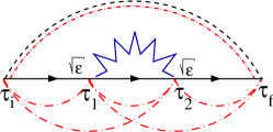
Figure 1: First and second order Feynman diagrams contributing to electron’s GF. Solid line represents ${\cal G}^{[0]}_{\alpha,\sigma}$; double dashed line stands for combination of Coulomb and longitudinal bosons; single dashed line denotes a longitudinal boson while the zig-zag line represents $\langle\Phi^{+}(\tau_{1})\Phi^{-}(\tau_{2})\rangle$.

In the spirit of Kam96 , the interaction of electrons with the finite-frequency charge and longitudinal modes ($\phi_{n}$, $\Phi^{z}_{n}$) may be interpreted in terms of a gauge boson com5 dressing the electron propagator (cf Fig.1a). The exact electronic GF (depending on winding numbers Efetov ) is given by Kam96

$${\cal G}_{\alpha,\sigma}(\tau_{i}-\tau_{f})={\cal G}^{[0]}_{\alpha,\sigma}(\tau_{i}-\tau_{f},\tilde{\mu})e^{-S_{\parallel}(\tau_{i}-\tau_{f})},$$ (20)

where the Coulomb-longitudinal $U$$($$1$$)$ gauge factor is

$$S_{\parallel}(\tau)=4T\sum_{n\neq 0}\frac{E_{c}-J/4}{\omega_{n}^{2}}\sin^{2}\left(\frac{\omega_{n}\tau}{2}\right)=$$

$$=\left(E_{c}-\frac{J}{4}\right)\left(|\tau|-\frac{\tau^{2}}{\beta}\right).$$ (21)

The exchange interaction effectively modifies the charging energy. For long-range interaction this correction is small $E_{c}/J$$\sim$$(k_{F}L)^{d-1}$ review ($L$ is a linear size of the $d$-dimensional confined electron gas, $k_{F}$ is a Fermi momentum), while for contact interaction $E_{c}-J/4=0$ review .

Transverse fluctuations. The first non-vanishing diagram of our expansion (18) is depicted in Fig.1b. Here

$${\cal G}^{[0]}_{\alpha,\sigma}(\tau)=e^{-\xi_{\alpha\sigma}\tau}\left(n_{\xi_{\alpha\sigma}}(1-\theta_{\tau})-(1-n_{\xi_{\alpha\sigma}})\theta_{\tau}\right)\;\;\;\;$$ (22)

the transverse correlator is considered in the Gaussian approximation

$$\langle\Phi^{+}(\tau_{1})\Phi^{-}(\tau_{2})\rangle=\frac{J}{2}\delta\left(\tau_{1}-\tau_{2}\right)+\frac{\epsilon J^{2}}{\displaystyle 2\beta(\Delta-\epsilon J)}.$$ (23)

In Eq.(23) the first term is a manifestation of the white noise fluctuations of the fields $\vec{\Phi}$ arising from the Gaussian weight factor (cf. Eq. (19)). The second term is related to the non-Gaussian factor in ${\cal D}^{\mu\nu}$ and reflects the feed-back of (the ${\cal D}$-dependent) ${\cal G}^{[0]}$ on ${\cal D}$. Note that the transverse components $\Phi^{\pm}$ are always accompanied by the gauge factors $e^{\mp 2\eta}$, hence the longitudinal bosons contribute to the dynamics involving the transverse fluctuations.

To proceed we now sum Eq.(18) over $\alpha$. Perturbative corrections to the electron GF coming from transverse fluctuations are now expanded in $\epsilon$ and summed up in the factor $F_{\perp}$

$$G(\tau)=G_{0}(\tau)e^{-S_{\parallel}(\tau)}F_{\perp}(\tau,\epsilon),$$ (24)

where

$$F_{\perp}(\tau,\epsilon)=1+\sum_{n,m}\{f^{(n)}g^{(m)}\}.$$ (25)

The effects of disorder are incorporated in the bare density of states $\nu_{0}=1/\Delta$. We denote $\tau$$\equiv$$\tau_{f}$$-$$\tau_{i}$. At finite temperatures we employ the conformal transformation $1/(\tau_{i}-\tau_{f})\to\pi/(\beta\sin\left(\pi(\tau_{i}-\tau_{f})/\beta\right))$. The factors $\{f^{(n)}g^{(m)}\}$ refer to diagrams containing $n+m$ ${\cal D}$ (zig-zag) line correlators, in $n$ $(m)$ of which we employ the first, $\delta$-function (second, constant) term of Eq. (23). The $\{f^{(n)}g^{(m)}\}$ factor is $\sim\epsilon^{n+2m}$. Here we calculate $F_{\perp}$ to order $\epsilon^{2}$.

In general, we may write the effective transverse gauge boson as $D_{\perp}(\epsilon,\tau)=\exp\left(-S_{\perp}(\epsilon,\tau)\right)$ exponentiation . $S_{\perp}$ preserves the symmetry (in $\tau$) with respect to $\beta/2$ to all orders of $\epsilon$. It can therefore be written as $S_{\perp}(\epsilon,\tau-\frac{\tau^{2}}{\beta})$.

The first term in (25) (of order $\epsilon$) is given by

$$f^{(1)}=\epsilon\frac{J}{2}\left(\tau-\frac{\tau^{2}}{\beta}\right)$$ (26)

This contribution is of the same origin as that of the longitudinal boson part (namely it comes from the $\frac{1}{J}\int_{0}^{\beta}\vec{\Phi}^{2}d\tau$ term in Eq. (23).) Along with the other $m=0$ terms in (25) it can be exponentiated exponentiation , resulting in $J/4\to J(1+2\epsilon)/4$ in the expression for $S_{\parallel}$. For the isotropic model one obtains $(1+2\epsilon)/4\to S(S+1)$.

There are contributions to $S_{\perp}$ arising from the second term of Eq.(23). As a result, the lowest, $\sim\epsilon^{2}$ contribution (the $\{f^{(0)}g^{(1)}\}$ term of the expansion (25)) leads to a non-Gaussian contribution to $S_{\perp}$ which is $\sim-\frac{\epsilon^{2}J^{2}}{\displaystyle 2\beta(\Delta-\epsilon J)}[\tau-\frac{\tau^{2}}{\beta}]^{2}$. It is easy to show that below the incipient Stoner instability, $J$$<$$J_{c}$, $S_{\perp}$ is dominated by the ”white noise” term of Eq.(23), while above this point it is the second (singular Stoner) term in (23) which dominates.

Tunneling density of states. The conductance $g_{T}$ is related to the tunnelling DoS $\nu$ through $g_{T}=\displaystyle\frac{e}{\hbar}\int d\epsilon\nu(\epsilon)\Gamma(\epsilon)\left(-\frac{\partial f_{F}}{\partial\epsilon}\right)$ where $f_{F}$ is the Fermi distribution function at the contact and $\Gamma$ is the golden rule dot-lead broadening. To obtain the TDoS from the GF, Eq.(24), we deform the contour of integration in accordance with Kam96 . As a result, the TDoS is given by Mat02

$$\nu(\epsilon)=-\frac{1}{\pi}\cosh\left(\frac{\epsilon}{2T}\right)\int_{-\infty}^{\infty}\sum_{\sigma}\langle G_{\sigma}\left(\frac{1}{2T}+it\right)\rangle_{k,m}e^{i\epsilon t}dt.$$ (27)

where $\langle...\rangle_{k,m}$ denotes a summation over all winding numbers for Coulomb and longitudinal zero-modes Efetov . We have computed the temperature and energy dependence of the TDoS for various values of $\epsilon$. These are depicted in Fig.2. The energy dependent TDoS shows an intriguing non-monotonic behavior at energies comparable to the charging energy $E_{c}$. This behavior, absent for $J=0$, is due to the contribution of the second term in Eq.(23). It is amplified in the vicinity of the Stoner point, and signals the effect of collective spin excitations (incipient ordered phase).

Spin susceptibilities. The spin susceptibilities are defined through

$$\chi^{\mu\nu}(\tau_{i},\tau_{f})=\frac{\partial^{4}{\cal Z}}{\partial\bar{\Lambda}^{\mu}_{\tau_{f}}\partial\Lambda^{\nu}_{\tau_{f}}\partial\bar{\Lambda}^{\nu}_{\tau_{i}}\partial\Lambda^{\mu}_{\tau_{i}}}$$ (28)

The longitudinal susceptibility ($\chi^{zz})$ is not affected by the gauge bosons. By contrast, the transverse $\chi^{+-}$ acquires the gauge factor $\langle$$e^{2\eta(\tau)}$$\rangle_{m,\Phi^{z}}$, where the average is performed with respect to the Gaussian fluctuations of $\Phi^{z}$ and, in principle, the winding numbers (cf. Eq.(16)). In practice, since $T$$>$$J$, only the $m=0$ winding should be taken into account; $T$$>$$\Delta$ allows us to evaluate the path integral in the Gaussian approximation. One finds to leading order in $\epsilon$

$$\chi^{zz}(\tau)=\frac{\chi_{0}}{1-J\chi_{0}},\;\;\;\;\;\chi^{+-}(\tau)=\frac{\epsilon\chi_{0}e^{J\tau}}{1-\epsilon J\chi_{0}}$$ (29)

where $\chi_{0}=1/\Delta$. The above susceptibilities are given as function of $\tau$. To obtain the dynamic susceptibilities one needs to Fourier transform and then continue to real frequencies. $\chi^{zz}$ (29) shek diverges at the thermodynamic Stoner Instability point, while $\chi^{+-}$ remains finite. Notwithstanding, the static transverse susceptibility is enhanced by the gauge fluctuations. The dynamic behavior (including relaxation processes) and the $\epsilon$ corrections to $\chi^{\mu\nu}$ will be discussed elsewhere.unp .

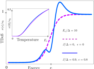
Figure 2: The spin-normalized tunneling density of states shown as function of energy. Insert: TDoS as function of temperature.

Summarizing, we investigate influence of spin and charge zero-mode interactions on the TDoS and the susceptibilities. Longitudinal spin fluctuations suppress the CB and the static longitudinal susceptibility is greatly enhanced near the Stoner instability. Transverse fluctuations generally tend to suppress the CB, but also contain a term which dominates the dynamics near the Stoner instability and enhances the CB. The transverse susceptibility will be enhanced as well. On a more technical level, Coulomb interaction is described in terms of Abelian (U(1)) gauge theory and lead to Gaussian gauge factor, the spin interaction, being a subject of non-Abelian (SU(2)) gauge gives rise to non-Gaussian gauge factors.

We are acknowledge useful discussions with Y.Alhassid, L.Glazman, I.V. Lerner, K.Matveev, A.Mirlin and Z.Schuss. We acknowledge support by SFB-410 grant, the Transnational Access program RITA-CT-2003-506095 (MK), an ISF grant of the Israel Academy of Science, the EC HPRN-CT-2002-00302-RTN and the AvH Foundation (YG). We are grateful to Argonne National Laboratory for the hospitality during our visit. Research in Argonne was supported by U.S. DOE, Office of Science, under Contract No. W-31-109-ENG-39.

References

• (1) I.L.Kurland, I.L.Aleiner, and B.L.Altshuler, Phys. Rev B 62, 14 886 (2000).
• (2) I.L.Aleiner, P.W.Brouwer, L.I.Glazman, Phys. Rep. 358, 309 (2002).
• (3) E.C.Stoner, Rep. Prog. Phys. 11, 43 (1947).
• (4) D.Weinmann, W.Häusler, and B.Kramer, Phys. Rev. Lett.74, 984 (1995).
• (5) Y.Alhassid and T.Rupp, Phys. Rev. Lett. 91, 056801 (2003).
• (6) I.O.Kulik and R.I.Shekhter, JETP 41, 308 (1974); E.Ben-Jacob and Y.Gefen, Phys. Lett. 108A, 289 (1985).
• (7) A.Kamenev and Y.Gefen, Phys.Rev. B 54, 5428 (1996).
• (8) There are several possible sources for such anisotropy, e.g., geometrical anisotropy, molecular anisotropy and spin-orbit interaction. The degree of anisotrpy can be controlled by introducing magnetic impurities into the system, or by applying anisotrpic mechanical pressure (see e.g., J.Kanamori, Magnetism (eds. G.T.Rado and H.Suhl), 1 N.Y.501 (1966)).
• (9) As both $J$ and $\Delta$ are inversely proportional to the volume of the system, the spin of the ground state scales as $S_{g}\sim\left[\epsilon J/(\Delta-J)\right]$.
• (10) This criterion generalizes the results of Ref. Hamiltonian for the case of an easy-axis anisotropy. In the isotropic case it reads $J^{even}_{c}=\Delta/2$, $J_{c}^{odd}=2\Delta/3$, whereas for the Ising case one has $J^{even}_{c}=J_{c}^{odd}=J_{th}=\Delta$.
• (11) K.B.Efetov and A.Tschersich, Phys.Rev. B 67, 174205 (2003); N.Sedlmayer, I.V. Yurkevich and I. V. Lerner, unpublished. We thank I.Beloborodov, I. V. Lerner and I.V. Yurkevich for discussions on this point.
• (12) $\phi_{n}$, $\vec{\Phi}_{n}$ denote the $n$-th Matsubara components.
• (13) The exponential gauge factor being continuous at points $\tau=0,\beta$ does not, strictly speaking, correspond to a bosonic propagator. We, nevertheless, keep the terminology of Kam96 .
• (14) The transverse gauge boson is given by $D_{\perp}(\tau)$ $=$ $\exp$ $\left(-S_{\perp}(\tau)\right)$, where $S_{\perp}(\tau)$ $=$ $-\ln$ $\left[1+\sum_{n,m}\{f^{(n)}g^{(m)}\}\right]$.
• (15) K.A.Matveev and A.V.Andreev, Phys. Rev. B 66, 045301 (2002).
• (16) The longitudinal susceptibility has been analyzed in a different regime by M.Schechter, Phys.Rev. B 70, 024521 (2004).
• (17) Y.Gefen and M.Kiselev (unpublished).