Fluctuation theorem for non-equilibrium relaxational systems
driven by external forces

Abstract

We discuss an extension of the fluctuation theorem to stochastic models that, in the limit of zero external drive, are not able to equilibrate with their environment, extending results presented by Sellitto (cond-mat/9809186). We show that if the entropy production rate is suitably defined, its probability distribution function verifies the Fluctuation Relation with the ambient temperature replaced by a (frequency-dependent) effective temperature. We derive modified Green-Kubo relations. We illustrate these results with the simple example of an oscillator coupled to a nonequilibrium bath driven by an external force. We discuss the relevance of our results for driven glasses and the diffusion of Brownian particles in out of equilibrium media and propose a concrete experimental strategy to measure the low frequency value of the effective temperature using the fluctuations of the work done by an ac conservative field. We compare our results to related ones that appeared in the literature recently.

I Introduction

Relatively few generic results for non-equilibrium systems exist. Recently, two such results that apply to seemingly very different physical situations have been proposed and extensively studied. One is the fluctuation theorem that characterizes the fluctuations of the entropy production over long time-intervals in certain driven steady states ECM93 ; GC95a . Another one is the extension of the fluctuation–dissipation theorem that relates induced and spontaneous fluctuations in equilibrium to the non-equilibrium slow relaxation of glassy systems Cuku93 ; Cuku . While the former result has been proven for reversible hyperbolic dynamical systems GC95a ; GC95b and for the driven stochastic dynamic evolution of an open system coupled to an external environment Ku98 ; LS99 , the latter has only been obtained in a number of solvable mean-field models and numerically in some more realistic glassy systems (see Felix-review for a review). The modification of the fluctuation–dissipation theorem can be rationalized in terms of the generation of an effective temperature Cukupe ; Cukuja . The expected thermodynamic properties of the effective temperature have been demonstrated in a number of cases proviso .

One may naturally wonder whether these two quite generic results may be included in a common, more general statement. The scope of this article is to discuss this possibility in general, illustrating it with a very simple example in which one can very easily reach the ‘driven limit’ and the ‘non-equilibrium relaxational’ case. This project was pioneered by Sellitto Se98 who asked the same question some years ago and tried to give it an answer using a stochastic lattice gas with reversible kinetic constraints in diffusive contact with two particle reservoirs at different chemical potentials. Other developments in similar directions have been proposed and analyzed by several authors SCM04 ; CR04 ; Sasa . We shall discuss them in Sect. VIII.

Before entering into the details of our calculations let us start by reviewing the precise statement of the usual fluctuation theorem and the extension of the fluctuation–dissipation theorem as well as the definition of the effective temperature.

I.1 The fluctuation theorem

The fluctuation theorem concerns the fluctuations of the entropy production rate comment1 , that we call $\sigma(x)$, in the stationary non-equilibrium state of a dynamical system defined by a state variable $x\in M$, where $M$ is the phase space of the system.

In non-equilibrium stationary states the function $\sigma(x)$ has a positive average, $\sigma_{+}=\int_{M}dx\mu_{+}(x)\sigma(x)>0$, where $\mu_{+}(x)$ is the stationary state distribution. This allows one to define

$$p(x)\equiv\frac{1}{{\tau}\sigma_{+}}{\cal{S}}_{\tau}=\frac{1}{{\tau}\sigma_{+}}\int_{-{\tau}/2}^{{\tau}/2}dt\ \sigma(S_{t}x)\ ,$$ (1)

where $S_{t}x$, with time $t\in[-{\tau}/2,{\tau}/2]$, is a segment of the system’s trajectory starting at the point $x$ at $t=-{\tau}/2$. The large deviation function of $p(x)$ is

$$\zeta(p)=\lim_{{\tau}\rightarrow\infty}{\tau}^{-1}\ln\pi_{\tau}(p)\ ,$$ (2)

where $\pi_{\tau}(p)$ is the distribution of $p$ in the stationary non-equilibrium state. The fluctuation theorem is the following statement about the large deviation function of $p(x)$:

$$\zeta(p)-\zeta(-p)=p\sigma_{+}\ .$$ (3)

The relation (3) was first discovered in a numerical simulation ECM93 , and subsequently stated as a theorem for reversible hyperbolic dynamical systems (the Gallavotti-Cohen Fluctuation Theorem) GC95a ; GC95b . The proof was extended to Langevin systems coupled to a white bath in Ku98 and to generic Markov processes in LS99 . Equation (3) was successfully tested in a wide number of numerical simulations, see e.g. BGG97 ; BCL98 ; GRS04 ; ZRA04a , and, more recently, it was also analyzed in experiments on granular materials and turbulent flows CL98 ; GGK01 ; CGHLP03 ; FM04 . At present, it is believed to yield a very general characterization of the fluctuations of the entropy production in a variety of out of equilibrium stationary states.

In all the cases cited above an external drive maintains the systems in a stationary non-equilibrium regime. In the absence of the drive the systems so far analyzed easily equilibrate. In the stochastic case, the systems are in contact with an equilibrated environment at a well-defined temperature.

I.2 The effective temperature

The analytic solution to the relaxation of mean-field glassy models following a quench into their glassy phase demonstrated that their relaxation occurs out of equilibrium Cuku93 ; Cuku . The reason why these models do not reach equilibrium when relaxing from a random initial condition is that their equilibration time diverges with their size. Thus, when the thermodynamic limit is taken at the outset of the calculation, all times considered are finite with respect to the size of the system. These systems approach a slow nonequilibrium regime in which one observes a breakdown of stationarity and, more importantly for the subject of this paper, a violation of the fluctuation-dissipation theorem that relates spontaneous and induced fluctuations in thermal equilibrium.

The relation between spontaneous and induced fluctuations found in mean-field glassy models is, however, surprisingly simple. Let us define the linear response of a generic observable $O$ measured at time $t$ to an infinitesimal perturbation constantly applied since a previous ‘waiting-time’ $t_{w}$, and the correlation between the same (unperturbed) observable measured at $t_{w}$ and $t$,

$$\chi(t,t_{w}) \equiv \int_{t_{w}}^{t}dt^{\prime}\;R(t,t^{\prime})=\int_{t_{w}}^{t}dt^{\prime}\;\left.\frac{\delta\langle O(t)\rangle}{\delta h(t^{\prime})}\right|_{h=0}\;,$$ (4)

$$C(t,t_{w}) \equiv \langle O(t)O(t_{w})\rangle\;,$$ (5)

where, for simplicity, we assumed that the observable $O$ has a vanishing average, $\langle O(t)\rangle=0$ for all $t$. In the cases we shall be interested in the relation between these two quantities takes the form

$$\lim_{t_{w}\gg t_{0}}\chi(t,t_{w})=f[C(t,t_{w})]$$ (6)

in the long waiting-time limit after the initial time $t_{0}$. This equation means that the waiting-time and total time dependence in $\chi$ enters only through the value of the associated correlation between these times. This is trivially true in equilibrium since the fluctuation-dissipation theorem states

$$f(C)=\frac{1}{T}\;(1-C)\;,$$ (7)

for all times $t\geq t_{w}\geq t_{eq}$, where $T$ is the temperature of the thermal bath (and the one of the system as well) and we set the Boltzmann constant to one, $k_{B}=1$. Out of equilibrium $f(C)$ can take a different form. In a large variety of models with slow dynamics that describe aspects of glasses $f(C)$ is a broken line,

$$f(C)=\frac{1}{T}\;(1-C)\;\theta(C-q_{ea})+\left[\frac{1}{T}\;(1-q_{ea})+\frac{1}{T_{eff}}(q_{ea}-C)\right]\;\theta(q_{ea}-C)\;,$$ (8)

see Felix-review for a review. This broken line has two slopes, $-1/T$ for $C>q_{ea}$ (i.e., small $t-t_{w}$), and $-1/T_{eff}$ for $C<q_{ea}$ (i.e., large $t-t_{w}$). The breaking-point $q_{ea}$ has an interpretation in terms of intra-cage and out-of-the cage motion in the relaxation of structural glasses, inter-domain and domain wall motion in coarsening systems, etc. Since $T_{eff}$ is found to be larger than $T$ the second term violates the fluctuation-dissipation theorem. We have used the suggestive name effective temperature, $T_{eff}$, to parametrize the second slope. The justification is that for mean-field glassy models — and within all resummation schemes applied to realistic ones as well — $T_{eff}$ does indeed behave as a temperature Cukupe . A similar relation was later found numerically in the slow relaxational dynamics of a number of more realistic glassy systems such as Lennard-Jones mixtures Lennard-FDT . More complicated forms, with a sequence of segments with different slopes appear in mean-field glassy models of the Sherrington-Kirkpatrick type.

The general definition of the effective temperature is

$$-\frac{1}{T_{eff}(C)}=\frac{d\chi}{dC}\;.$$ (9)

In order to be consistent with the thermodynamic properties one needs to find a single value of $T_{eff}$ in each time regime as defined by the correlation scales of Ref. Cuku .

So far we considered systems relaxing out of equilibrium in the absence of external drive. The extension of the definition of the effective temperature to the driven dynamics of glasses and super-cooled liquids was again motivated by the analytic solution of mean-field models under non-potential forces Cukulepe ; Cukulepe1 ; BBK00 . The existence of non-trivial effective temperatures, i.e. of functions $f(C)$ that differ from Eq. (7), was also observed in numerical simulations of sheared Lennard-Jones mixtures BB00 ; BB02 and in a number of other driven low-dimensional models lowd-driven .

In the case of relaxing glasses the dynamics occurs out of equilibrium because below some temperature the equilibration time falls beyond all experimentally accessible time-scales. These macroscopic systems then evolve out of equilibrium even if they are in contact with a thermal reservoir, itself in equilibrium at a given temperature $T$. Under the effect of stirring forces, supercooled liquids and glasses are typically driven into a nonequilibrium stationary regime, even for relatively modest flow.

I.3 A connection between the two?

The fluctuation theorem and the fluctuation–dissipation theorem are related: indeed, it was proven that, for systems which are able to equilibrate in the small entropy production limit ($\sigma_{+}\rightarrow 0$), the fluctuation theorem implies the Green-Kubo relations for transport coefficients, that are a particular instance of the fluctuation–dissipation theorem Ga96a ; Ga96b ; Ku98 .

It is now natural to wonder what is the fate of the fluctuation theorem if the system on which the driving force is applied cannot equilibrate with its environment and evolves out of equilibrium even in the absence of the external drive. Our aim is to investigate whether the fluctuation theorem is modified and, more precisely, whether the effective temperature Cukupe enters its modified version. In particular, this question will arise if the limit of large sampling time, $\tau$ in Eqs. (1) and (2), is taken after the limit of large system size. The order of the limits is important because a finite size undriven system will always equilibrate with the thermal bath in a large enough time $\tau$. As the fluctuation theorem concerns the fluctuations of $\sigma$ for $\tau\to\infty$, if one wants to observe intrinsic nonequilibrium effects, the latter limit has to be taken after the thermodynamic limit. Some conjectures about this issue have recently appeared in the literature CR04 ; SCM04 ; Se98 ; Sasa and we discuss them in Sect. VIII.

Our idea is to study the relaxational and driven dynamics of simple systems such that the effective temperature is not trivially equal to the ambient temperature. For a system coupled to a single thermal bath, this happens whenever:

(i) the thermal bath has temperature $T$, but the system is not able to equilibrate with the bath. This is realized by the glassy cases discussed above, provided the sampling time is smaller than the equilibration time; and/or

(ii) the system is very simple (not glassy) but it is set in contact with a bath that is not in equilibrium. One can think of two ways of realizing this. One is with a single bath represented by a thermal noise and a memory friction kernel that do not verify the fluctuation-dissipation relation Cu02 . This situation arises if one considers the diffusion of a Brownian particle in a complex medium (e.g. a glass, or granular matter) PM04 ; Po04 ; AG04 . In this case the medium, which acts as a thermal bath with respect to the Brownian particle, is itself out of equilibrium. Another example is the one of a system coupled to a number of equilibrated thermal baths with different time-scales and at different temperatures Cukuja .

I.4 Effective equations for the dynamics of mean-field glasses

The cases (i) and (ii) mentioned in the previous section are closely related as, at least at the mean-field level, the problem of glassy dynamics can be mapped onto the problem of a single “effective” degree of freedom moving in an out of equilibrium self-consistent environment Cu02 ; Cukuja . Situations (i) and (ii) are then described by the same kind of equation, namely, a Langevin equation for a single degree of freedom coupled to a non-equilibrium bath.

Indeed, in the study of mean-field models for glassy dynamics Cu02 ; Cukuja and when using resummation techniques within a perturbative approach to microscopic glassy models with no disorder, it is possible to reduce the $N$-dimensional equations of motion to a single equation for an ‘effective’ variable by means of a saddle-point evaluation of the dynamic generating functional. These equations are valid in the large size $N\to\infty$ limit; the discussion that follows concerns the fluctuation relation involving ${\cal{S}}_{\tau}$ for $\tau\rightarrow\infty$ taken after $N\to\infty$: for these finite timescales $\tau$ a fluctuation relation involving effective temperatures may and will arise, while for the extreme times $\tau\rightarrow\infty$ before $N\to\infty$ the usual fluctuation theorem (involving only the bath temperature $T$) holds.

The effective equation of motion of a single spin at finite time reads

$$\gamma\dot{\varphi}_{t}=-\mu(t)\ \varphi_{t}+\int_{-\infty}^{t}dt^{\prime}\ \Sigma(t,t^{\prime})\ \varphi_{t^{\prime}}+\rho_{t}+\alpha h[\varphi_{t}]\ ,$$ (10)

where $\rho_{t}$ is a Gaussian noise such that $\langle\rho_{t}\rho_{t^{\prime}}\rangle=D(t,t^{\prime})$. The “self-energy” $\Sigma(t,t^{\prime})$ and the “vertex” $D(t,t^{\prime})$ depend on the interactions in the system. They cannot be calculated exactly for generic interactions but they can be approximated within different resummation schemes (mode-coupling, self-consistent screening, etc.) or calculated explicitly for disordered mean-field models. The last term (if present) represents an external drive.

In the absence of the driving force Eq. (10) shows a dynamical transition at a temperature $T_{d}$. Above $T_{d}$, in the limit $t,t^{\prime}\rightarrow\infty$ the functions $\Sigma(t,t^{\prime})$ and $D(t,t^{\prime})$ become time-translation invariant and are related by the fluctuation-dissipation relation with $\Sigma$ playing the role of a response and $D$ being a correlation. Below $T_{d}$ the system is no more able to equilibrate with the thermal bath and ages indefinitely, i.e. the functions $\Sigma(t,t^{\prime})$ and $D(t,t^{\prime})$ depend on $t$ and $t^{\prime}$ separately even in the infinite time limit, and the relaxation time $\tau_{\alpha}$ grows indefinitely. At low temperatures the fluctuation-dissipation theorem does not necessarily hold, and the relation between $\Sigma$ and $D$ can be used to measure the effective temperature for the particular problem at hand.

In the case of a driven mean field system Cukulepe ; Cukulepe1 ; BBK00 , the external force is also present in Eq. (10) and after a transient the system becomes stationary for any temperature, i.e. $\mu(t)\equiv\mu$, $\Sigma(t,t^{\prime})=\Sigma(t-t^{\prime})$, and $D(t,t^{\prime})=D(t-t^{\prime})$. The functions $D$ and $\Sigma$ depend on the strength $\alpha$ of the driving force. Below $T_{d}$ and for small $\alpha$ they are again related by a generalization of the fluctuation-dissipation theorem similar to the one obtained for $\alpha=0$.

In this paper we focus on Langevin equations similar to Eq. (10). Their main characteristic is that the thermal bath, represented by the functions $\Sigma(t,t^{\prime})$ and $D(t,t^{\prime})$, is not in equilibrium. As we are interested in the driven case, we restrict to considering stationary functions $\Sigma(t-t^{\prime})$ and $D(t-t^{\prime})$.

Let us remark that Eq. (10) is expected to describe the dynamics of a single Brownian particle immersed in a non–equilibrium environment, or the dynamics of an effective degree of freedom representing a many–particle mean–field glassy system. If one wishes to describe in full detail the relaxation of real glasses in finite dimensions, more complicated effects have to be taken into account. For example, the dynamics is expected to be heterogeneous yielding a local effective temperature which may depend on space inside the sample, see e.g. Cu04 for a detailed discussion. The extension of the results that we shall present in this paper to glassy systems in finite dimension might require additional work.

I.5 Summary and structure of the paper

The aim of this work is to discuss the validity of the fluctuation theorem for the Langevin equation (10) in presence of a non-trivial environment represented by the functions $\Sigma(t)$ and $D(t)$. This equation describes a situation in which the relaxing system does not equilibrate with its environment (even in the absence of driving forces) and a non-trivial effective temperature defined from the modification of the fluctuation-dissipation theorem exists. Our first aim is to identify the entropy production rate and to show that the effective temperature of the environment should replace the ambient temperature of a conventional bath.

As particular cases we investigate analytically the dynamics in a harmonic well and numerically a case in which the equations of motion are nonlinear. The former problem is relevant for experiments on confined Brownian particles in complex media AG04 ; Gr03 . In both cases we show that we show that the entropy production rate that we introduced verifies the fluctuation relation in general.

The paper is organized as follows. In section II we identify the correct definition of entropy production rate using a rather general procedure proposed by Lebowitz and Spohn. As an illustration, in section III we analytically compute the large deviation function in the harmonic case for a white equilibrium bath, already discussed in Ref. Ku98 , and for a complex bath. We show that the large deviation function is a convex function of $p$ and satisfies the fluctuation relation. In section IV we compare the analytic results obtained for the linear problem with numerical data. We also numerically investigate a nonlinear Langevin equation, in which the entropy production is not only given by the work of the external forces, but should contain an ‘internal’ term as well. Surprisingly, this term turns out to be negligible, a result we attribute to decorrelation between the work of internal and external forces. In section V we make contact with glassy problems and discuss some connections with recent numerical simulations. Section VI is devoted to the analysis of the link between the modified fluctuation theorem and modified Green-Kubo relations. In Section VII we show explicitely that the distribution of the work done by a slow periodic drive satisfies the fluctuation relation with the low-frequency effective temperature, and argue that this procedure is the one that could be “easily” implemented experimentally as a means to measure the (low frequency) effective tempeature. In the conclusions we briefly discuss some experiments that could test our predictions, and compare them to previous studies of the same problem.

II Entropy production

In this Section we introduce the set of dynamic models that we discuss in detail, namely, stochastic processes of generic Langevin type with additive noise. Next, we define the large deviation function that we shall use to test the validity of the fluctuation relation and, finally, we derive a general expression for the entropy production rate.

II.1 The model

In this article we focus on different aspects of the random motion of a particle in a confining potential, in contact with a thermal environment, and under the effect of a driving external force. The Langevin equation describing the motion of such a particle in a $d$ dimensional space reads

$$m\ddot{r}_{\alpha}(t)+\int_{-\infty}^{\infty}dt^{\prime}\;g_{\alpha\beta}(t-t^{\prime})\dot{r}_{\beta}(t^{\prime})=-\frac{\partial V}{\partial r_{\alpha}}[\vec{r}(t)]+\rho_{\alpha}(t)+h_{\alpha}(t)\;,\;\;\;\;\;\;\;\;\;\alpha=1,\dots,d\;.$$ (11)

${\vec{r}}=(r_{1},\dots,r_{d})$ is the position of the particle. We pay special attention to the case $d=2$ and call $(x,y)$ the two components of the position vector. $m$ is the mass of the particle and $V({\vec{r}})$ is a potential energy. As an example we shall work out in detail the simple harmonic case, $V({\vec{r}})=\frac{k}{2}\sum_{\alpha}r_{\alpha}^{2}$ with $k$ the spring constant of the quadratic potential. ${\vec{\rho}}(t)$ is a Gaussian thermal noise with zero average and generic stationary correlation

$$\langle\,\rho_{\alpha}(t)\rho_{\beta}(t^{\prime})\,\rangle=\delta_{\alpha\beta}\;\nu(t-t^{\prime})\;\;\;\;\;\;\;\;\;\alpha,\beta=1,\dots,d\;,$$ (12)

with $\nu(t-t^{\prime})$ a symmetric function of $t-t^{\prime}$. The memory kernel $g_{\alpha\beta}(t-t^{\prime})$ extends the notion of friction to a more generic case. We assume a simple spatial structure, $g_{\alpha\beta}(t-t^{\prime})=\delta_{\alpha\beta}\;g(t-t^{\prime})$. In order to ensure causality we take $g(t-t^{\prime})$ to be proportional to $\theta(t-t^{\prime})$. We define

$$g(t)=\theta(t)f(t)\qquad\mbox{with}\qquad f(t)\equiv g(t)+g(-t)\;.$$ (13)

The initial time $t_{0}$ has been taken to $-\infty$. ${\vec{h}}(t)$ is a time-dependent field that we either use to compute the linear response or represents the external forcing.

It will be useful to introduce Fourier transforms. We use the conventions

$$\rho(t)=\int_{-\infty}^{\infty}\frac{d\omega}{2\pi}\;e^{-i\omega t}\,\rho(\omega)\;,\;\;\;\;\;\;\;\;\;\;\;\;\;\;\rho(\omega)=\int_{-\infty}^{\infty}dt\;e^{i\omega t}\,\rho(t)\;.$$ (14)

The fluctuation-dissipation theorem states that for systems evolving in thermal equilibrium with their equilibrated environment the linear response is related to the correlation function of the same observable as

$$R(t)=-\frac{\theta(t)}{T}\frac{dC(t)}{dt}\;,\;\;\;\;\;\;\;\;\;\;\;\;\;\;\frac{dC(t)}{dt}=T[R(-t)-R(t)]\;,$$ (15)

see Eqs. (4) and (5) for the definitions of $R$ and $C$. Here and in what follows we set the Boltzmann constant to one, $k_{B}=1$. To write the second expression we used that $C(t)$ is an even function of $t$ (and $\dot{C}(t)$ is odd) and defined $\theta(0)\equiv 1/2$ (the same convention is used in the rest of the paper). After Fourier transforming the second expression becomes

$$\omega C(\omega)=2T\text{Im}R(\omega)\ ,$$ (16)

and the real part of $R(\omega)$ is related to $\text{Im}R(\omega)$ by the Kramers-Krönig relation.

The functions $g$ and $\nu$ are the integrated response and correlation of the bath, respectively. As will be discussed in detail in section III, if the bath is itself in equilibrium at a temperature $T$ they are related as

$$\frac{1}{T}=\frac{2\text{Re}g(\omega)}{\nu(\omega)}\;.$$ (17)

For an out of equilibrium bath we define the frequency dependent temperature

$$\frac{1}{T(\omega)}=\frac{2\text{Re}g(\omega)}{\nu(\omega)}\;,$$ (18)

and its inverse Fourier transform

$$T^{-1}(t)=\int_{-\infty}^{\infty}\frac{d\omega}{2\pi}\frac{2\text{Re}g(\omega)}{\nu(\omega)}e^{-i\omega t}=\int_{-\infty}^{\infty}dt^{\prime}\nu^{-1}(t-t^{\prime})f(t^{\prime})\;.$$ (19)

where

$$\nu^{-1}(t)=\int\frac{d\omega}{2\pi}\frac{1}{\nu(\omega)}e^{-i\omega t}\ .$$ (20)

Note that both $f(t)$ and $T^{-1}(t)$ are even functions of $t$. If the bath is in equilibrium at temperature $T$, $T^{-1}(t-t^{\prime})=\delta(t-t^{\prime})/T$. We shall assume throughout that $T^{-1}(t)$ goes to zero fast enough for large $t$.

The main result of this paper is that the fluctuation relation for the probability distribution function $\pi_{\tau}(p)$ holds for long times $\tau$:

$$\tau\sigma_{+}\;p\sim\ln\frac{\pi_{\tau}(p)}{\pi_{\tau}(-p)}\ ,$$ (21)

with

$${\cal{S}}_{\tau}=\tau\sigma_{+}p=\int_{-\tau/2}^{\tau/2}dt\int_{-\tau/2}^{\tau/2}dt^{\prime}\,T^{-1}(t-t^{\prime})\;\dot{r}_{\alpha}(t)\left[-\frac{\partial V}{\partial r_{\alpha}}[\vec{r}(t^{\prime})]+h_{\alpha}[\vec{r}(t^{\prime})]\right]\;.$$ (22)

II.2 Large deviation function

In the rest of this section we identify the entropy production rate for Eq. (11) following the procedure proposed by Lebowitz and Spohn LS99 .

The fluctuation relation is a symmetry property of the probability distribution function (pdf) of the entropy production rate $\sigma_{t}$ that can be also expressed as a symmetry of the large deviation function. Calling $\sigma_{+}$ the average value of $\sigma_{t}$, the pdf of the variable $p$ defined in Eq. (1) is defined as

$$\pi_{\tau}(p)={\cal P}\left[\frac{{\cal{S}}_{\tau}}{{\tau}\sigma_{+}}=p\right]={\tau}\sigma_{+}\langle\,\delta({\cal S}_{\tau}-p{\tau}\sigma_{+})\,\rangle\;,$$ (23)

where the angular brackets denote an average over the realizations of the noise. The large deviation function [normalized so that $\zeta(1)=0$ at the maximum] is given by

$$\zeta(p)=\lim_{{\tau}\rightarrow\infty}{\tau}^{-1}\ln\big{[}\pi_{\tau}(p)/\pi_{\tau}(1)\big{]}\;.$$ (24)

It is easier to compute the characteristic function

$$\phi(\lambda)=-\lim_{{\tau}\rightarrow\infty}{\tau}^{-1}\ln\langle\exp[-\lambda\sigma_{\tau}]\rangle\ ;$$ (25)

the latter being the Legendre transform of $\zeta(p)$. Indeed,

$$e^{-{\tau}\phi(\lambda)}=\langle e^{-\lambda\sigma_{\tau}}\rangle=\frac{\int dp\,e^{{\tau}[\zeta(p)-\lambda p\sigma_{+}]}}{\int dp\,e^{{\tau}\zeta(p)}}\sim\frac{e^{{\tau}\max_{p}[\zeta(p)-\lambda p\sigma_{+}]}}{e^{{\tau}\zeta(1)}}$$ (26)

so that, recalling that $\zeta(1)=0$ by construction,

$$\phi(\lambda)=-\max_{p}\,[\zeta(p)-\lambda p\sigma_{+}]\ .$$ (27)

The inversion of the Legendre transform yields

$$\zeta(p)=\min_{\lambda}\,[\lambda p\sigma_{+}-\phi(\lambda)]\ ,$$ (28)

and it is easy to check that the fluctuation relation is equivalent to $\phi(\lambda)=\phi(1-\lambda)$.

II.3 Internal symmetries and the fluctuation relation

Assume that there exists a map $I$ on the space of trajectories $r(t)$ such that $I^{2}=1$ and that the measure ${\cal D}r$ is inviariant under $I$, i.e. ${\cal D}Ir={\cal D}r$. Then, consider a segment of trajectory $r(t)$, $t\in[-\tau/2,\tau/2]$ and define

$${\cal S}_{\tau}=-\ln\frac{{\cal P}[Ir(t)]}{{\cal P}[r(t)]}\ ,$$ (29)

where ${\cal P}[r(t)]$ is the probability of observing $r(t)$, in the stationary state, for $t\in[-\tau/2,\tau/2]$ irrespectively of what happens outside the interval $[-\tau/2,\tau/2]$. It is easy to show that the pdf of ${\cal S}_{\tau}$ verifies the fluctuation theorem. Indeed

$$\langle e^{-\lambda{\cal S}_{\tau}}\rangle=\int{\cal D}r\,{\cal P}[r(t)]e^{-\lambda{\cal S}_{\tau}}=\int{\cal D}r\,{\cal P}[r(t)]^{1-\lambda}\,{\cal P}[Ir(t)]^{\lambda}=\int{\cal D}r\,{\cal P}[Ir(t)]^{1-\lambda}\,{\cal P}[r(t)]^{\lambda}=\langle e^{-(1-\lambda){\cal S}_{\tau}}\rangle\ .$$ (30)

Thus, if the limit

$$\phi(\lambda)=-\lim_{\tau\rightarrow\infty}\tau^{-1}\ln\langle e^{-\lambda{\cal S}_{\tau}}\rangle$$ (31)

exists, it verifies the relation $\phi(\lambda)=\phi(1-\lambda)$ from which the fluctuation relation for the pdf of ${\cal S}_{\tau}$ follows. Lebowitz and Spohn showed that the limit $\phi(\lambda)$ indeed exists for generic Markov processes and it is a concave function of $\lambda$. Moreover they showed that ${\cal S}_{\tau}$ can be identified with the entropy production rate –over the time interval $\tau$– in the stationary state up to boundary terms, i.e. terms that do not grow with $\tau$, if $I$ is chosen to be the time reversal, $Ir(t)=r(-t)$.

II.4 Entropy production rate

We are interested in the explicit form of ${\cal{S}}_{\tau}$ for the equation of motion (11) in the case in which $g_{\alpha\beta}(t)=\delta_{\alpha\beta}g(t)$ and $\vec{h}(t)=\vec{h}[\vec{r}(t)]$ is an external nonconservative force that does not explicitly depend on time: e.g., in $d=2$, $\vec{h}=\alpha(-y,x)$. Note that the functions $\nu(t)$ and $g(t)$ are such that $\nu(t)=\nu(-t)$ while $g(t)$ is proportional to $\theta(t)$, and both decay sufficiently rapidly in time. The probability distribution of the noise $\vec{\rho}(t)$ is

$${\cal P}[\vec{\rho}(t)]\propto\exp\left[-\frac{1}{2}\int dtdt^{\prime}\,\rho_{\alpha}(t)\nu^{-1}(t-t^{\prime})\rho_{\alpha}(t^{\prime})\right]\ ,$$ (32)

where $\nu^{-1}(t)$ is the operator inverse of $\nu(t)$, see Eq. (20). The probability distribution of $\vec{r}(t)$ is obtained substituting $\vec{\rho}(t)$ obtained from Eq. (11) in Eq. (32). One has

$$\begin{split}{\cal P}[\vec{r}(t)]\propto&\exp\left\{-\frac{1}{2}\int dtdt^{\prime}\,\left[m\ddot{r}_{\alpha}(t)+\int dt^{\prime\prime}g(t-t^{\prime\prime})\dot{r}_{\alpha}(t^{\prime\prime})+\frac{\partial V}{\partial r_{\alpha}}[\vec{r}(t)]-h_{\alpha}[\vec{r}(t)]\right]\right.\\ &\left.\times\;\nu^{-1}(t-t^{\prime})\left[m\ddot{r}_{\alpha}(t^{\prime})+\int dt^{\prime\prime\prime}g(t^{\prime}-t^{\prime\prime\prime})\dot{r}_{\alpha}(t^{\prime\prime\prime})+\frac{\partial V}{\partial r_{\alpha}}[\vec{r}(t^{\prime})]-h_{\alpha}[\vec{r}(t^{\prime})]\right]\right\}\ .\end{split}$$ (33)

After some algebra it is easy to see that

$$\begin{split}{\cal P}[\vec{r}(-t)]\propto&\exp\left\{-\frac{1}{2}\int dtdt^{\prime}\,\left[m\ddot{r}_{\alpha}(t)-\int dt^{\prime\prime}g(t^{\prime\prime}-t)\dot{r}_{\alpha}(t^{\prime\prime})+\frac{\partial V}{\partial r_{\alpha}}[\vec{r}(t)]-h_{\alpha}[\vec{r}(t)]\right]\right.\\ &\left.\times\;\nu^{-1}(t-t^{\prime})\left[m\ddot{r}_{\alpha}(t^{\prime})-\int dt^{\prime\prime\prime}g(t^{\prime\prime\prime}-t^{\prime})\dot{r}_{\alpha}(t^{\prime\prime\prime})+\frac{\partial V}{\partial r_{\alpha}}[\vec{r}(t^{\prime})]-h_{\alpha}[\vec{r}(t^{\prime})]\right]\right\}\ .\end{split}$$ (34)

To compute ${\cal{S}}_{\tau}$ we should consider the probability of a segment of trajectory $[-\tau/2,\tau/2]$ and then send $\tau$ to $\infty$, neglecting all boundary terms. As the functions $g(t)$ and $\nu(t)$ have short range, the trajectories $\vec{r}(t)$ decorrelate, say, exponentially fast in time and up to boundary contributions one can simply truncate the integrals in ${\cal P}[\vec{r}(t)]$ in $t,t^{\prime}\in[-\tau/2,\tau/2]$.

Let us now discuss the contributions to $-\ln{\cal P}[\vec{r}(-t)]+\ln{\cal P}[\vec{r}(t)]$ that do not trivially vanish. One has:

• a “kinetic” term of the form

  $$\begin{split}&\int dtdt^{\prime}\,\left[m\ddot{r}_{\alpha}(t)\nu^{-1}(t-t^{\prime})\int dt^{\prime\prime}g(t^{\prime\prime}-t^{\prime})\dot{r}_{\alpha}(t^{\prime\prime})+m\ddot{r}_{\alpha}(t)\nu^{-1}(t-t^{\prime})\int dt^{\prime\prime}g(t^{\prime}-t^{\prime\prime})\dot{r}_{\alpha}(t^{\prime\prime})\right]=\\ &=\int dtdt^{\prime}\,m\ddot{r}_{\alpha}(t)\nu^{-1}(t-t^{\prime})\int dt^{\prime\prime}f(t^{\prime}-t^{\prime\prime})\dot{r}_{\alpha}(t^{\prime\prime})=\int dtdt^{\prime}\,m\ddot{r}_{\alpha}(t)T^{-1}(t-t^{\prime})\dot{r}_{\alpha}(t^{\prime})\ .\end{split}$$ (35)

  If the bath is in equilibrium, this term trivially vanishes as it is the integral of the total derivative of the kinetic energy. But it also vanishes for a nonequilibrium bath. Indeed, by integrating by parts first in $t$ and then in $t^{\prime}$, we find

  $$\begin{split}&\int dtdt^{\prime}\,\ddot{r}_{\alpha}(t)T^{-1}(t-t^{\prime})\dot{r}_{\alpha}(t^{\prime})=-\int dtdt^{\prime}\,\dot{r}_{\alpha}(t)\frac{d}{dt}T^{-1}(t-t^{\prime})\dot{r}_{\alpha}(t^{\prime})=\\ &\int dtdt^{\prime}\,\dot{r}_{\alpha}(t)\frac{d}{dt^{\prime}}T^{-1}(t-t^{\prime})\dot{r}_{\alpha}(t^{\prime})=-\int dtdt^{\prime}\,\dot{r}_{\alpha}(t)T^{-1}(t-t^{\prime})\ddot{r}_{\alpha}(t^{\prime})=0\ .\end{split}$$ (36)

  where we used that $T^{-1}(t)$ is even and short ranged and we neglected boundary terms.

• a “friction” term of the form

  $$\frac{1}{2}\int dtdt^{\prime}dt^{\prime\prime}dt^{\prime\prime\prime}\,\left[\dot{r}_{\alpha}(t^{\prime\prime})g(t^{\prime\prime}-t)\nu^{-1}(t-t^{\prime})g(t^{\prime\prime\prime}-t^{\prime})\dot{r}_{\alpha}(t^{\prime\prime\prime})-\dot{r}_{\alpha}(t^{\prime\prime})g(t-t^{\prime\prime})\nu^{-1}(t-t^{\prime})g(t^{\prime}-t^{\prime\prime\prime})\dot{r}_{\alpha}(t^{\prime\prime\prime})\right]\ .$$ (37)

  This term vanishes because the function

  $$K(t^{\prime\prime}-t^{\prime\prime\prime})=\int dtdt^{\prime}\,g(t^{\prime\prime}-t)\nu^{-1}(t-t^{\prime})g(t^{\prime\prime\prime}-t^{\prime})$$ (38)

  is even in its argument as one can easily check.

• a “potential” term of the form

  $${\cal{S}}_{\tau}^{V} = -\int_{-\tau/2}^{\tau/2}dt\int_{-\tau/2}^{\tau/2}dt^{\prime}\int_{-\tau/2}^{\tau/2}dt^{\prime\prime}\,f(t-t^{\prime\prime})\dot{r}_{\alpha}(t^{\prime\prime})\nu^{-1}(t-t^{\prime})\frac{\partial V}{\partial r_{\alpha}}[\vec{r}(t^{\prime})]$$ (39)

  $$= -\int_{-\tau/2}^{\tau/2}dt\int_{-\tau/2}^{\tau/2}dt^{\prime}\,T^{-1}(t-t^{\prime})\dot{r}_{\alpha}(t)\frac{\partial V}{\partial r_{\alpha}}[\vec{r}(t^{\prime})]\ .$$

  This term is related to the work of the conservative forces. If the bath is in equilibrium, it vanishes being the total derivative of the potential energy. It vanishes also for a harmonic potential $V(\vec{r})=\frac{1}{2}kr^{2}$ because $\frac{\partial V}{\partial r_{\alpha}}[\vec{r}(t)]=kr_{\alpha}(t)$ and one can use the same trick used in Eq. (36). It does not vanish in general.

• a “dissipative” term

  $${\cal{S}}_{\tau}^{diss}=\int_{-\tau/2}^{\tau/2}dt\int_{-\tau/2}^{\tau/2}dt^{\prime}\,T^{-1}(t-t^{\prime})\dot{r}_{\alpha}(t)h_{\alpha}[\vec{r}(t^{\prime})]\;.$$ (40)

  This term is related to the work of the dissipative forces. If the bath is in equilibrium at temperature $T$, this is exactly the work of the dissipative forces divided by the temperature of the bath. Otherwise, the work done at frequency $\omega$ is weighted by the effective temperature at the same frequency.

The expression of the total entropy production over the interval $[-\tau/2,\tau/2]$ is then

$${\cal{S}}_{\tau} = {\cal{S}}_{\tau}^{V}+{\cal{S}}_{\tau}^{diss}=\int_{-\tau/2}^{\tau/2}dt\int_{-\tau/2}^{\tau/2}dt^{\prime}\,T^{-1}(t-t^{\prime})\dot{r}_{\alpha}(t)\left[-\frac{\partial V}{\partial r_{\alpha}}[\vec{r}(t^{\prime})]+h_{\alpha}[\vec{r}(t^{\prime})]\right]$$ (41)

$$= \int_{-\tau/2}^{\tau/2}dt\int_{-\tau/2}^{\tau/2}dt^{\prime}\,T^{-1}(t-t^{\prime})\dot{r}_{\alpha}(t)F_{\alpha}(t^{\prime})\;,$$

where $F_{\alpha}(t)=h_{\alpha}[\vec{r}(t)]-\frac{\partial V}{\partial r_{\alpha}}[\vec{r}(t)]$ is the total deterministic force acting on the particle at time $t$.

The latter expression can be rewritten as

$${\cal{S}}_{\tau}\sim\int_{-\tau/2}^{\tau/2}dt\;\sigma_{t}=\int_{-\tau/2}^{\tau/2}dt\;(\sigma_{t}^{V}+\sigma_{t}^{diss})$$ (42)

defining a entropy production rates $\sigma_{t}$, $\sigma_{t}^{V}$ and $\sigma_{t}^{diss}$ (modulo subdominant terms in the large $\tau$ limit) as

$$\begin{split}&\sigma_{t}=\sigma^{V}_{t}+\sigma^{diss}_{t}=\int_{-\infty}^{t}dt^{\prime}\,T^{-1}(t-t^{\prime})\big{[}\dot{r}_{\alpha}(t)F_{\alpha}(t^{\prime})+\dot{r}_{\alpha}(t^{\prime})F_{\alpha}(t)\big{]}\ ,\\ &\sigma^{V}_{t}=-\int_{-\infty}^{t}dt^{\prime}\,T^{-1}(t-t^{\prime})\left[\dot{r}_{\alpha}(t)\frac{\partial V}{\partial r_{\alpha}}[\vec{r}(t^{\prime})]+\dot{r}_{\alpha}(t^{\prime})\frac{\partial V}{\partial r_{\alpha}}[\vec{r}(t)]\right]\ ,\\ &\sigma^{diss}_{t}=\int_{-\infty}^{t}dt^{\prime}\,T^{-1}(t-t^{\prime})\big{[}\dot{r}_{\alpha}(t)h_{\alpha}[\vec{r}(t^{\prime})]+\dot{r}_{\alpha}(t^{\prime})h_{\alpha}[\vec{r}(t)]\big{]}\ .\end{split}$$ (43)

We recall that if the bath is in equilibrium this expression reduces to the work done by the nonconservative forces divided by the temperature of the bath, as expected. If the bath is not in equilibrium, but the potential is harmonic, only the contribution $\sigma^{diss}_{\tau}$ of the nonconservative force has to be taken into account. The reason why the work of the conservative forces produces entropy if the bath is out of equilibrium and the interaction is nonlinear is that the nonlinear interaction couples modes of different frequency which are at different temperature, thus producing an energy flow between these modes; this energy flow is related to the entropy production.

It is also important to remark that boundary terms, that are usually neglected, can have dramatic effects on the large fluctuations of ${\cal S}_{\tau}$ even for $\tau\to\infty$, as pointed out by Van Zon and Cohen VzC04 . This happens if the pdf of the boundary term has exponential tails. Thus, boundary terms cannot be always neglected, at least for very large values of $p$. A good empirical prescription to remove boundary contributions is the following: in equilibrium $\sigma_{t}$ must be a total derivative as no dissipation is present. So, removing a total derivative (a boundary term) one can define ${\cal S}_{\tau}$ in such a way that it vanishes identically in equilibrium. This definition turns out to be the one that verifies the fluctuation relation for all $|p|<p^{*}$, $p^{*}$ being the maximum allowed value of $p$ for $\tau\to\infty$ VzC04 ; BGGZ05 . We shall discuss this point in more detail later.

III A driven particle in a harmonic potential

In this and the next Section we discuss some examples on which we test the fluctuation relation for ${\cal S}_{\tau}$ defined in (41). We first consider the simplest fully analytically solvable case in which there are no applied forces and the potential is quadratic. We derive the fluctuation-dissipation relation between induced and spontaneous fluctuations in the position of the particle and we relate it to the time-dependent temperature of the bath defined in Eq. (19). We then show that in this simple case the fluctuation relation for ${\cal S}_{\tau}$ in (41) reduces to the usual one with the temperature of the bath.

III.1 The fluctuation-dissipation relation

In the harmonic Brownian particle problem with no other applied external forces the dynamics of different spatial components are not coupled. Thus, without loss of generality, we henceforth focus on $d=1$. In Fourier space, the Langevin equation reads

$$-m\omega^{2}x(\omega)-i\omega g(\omega)x(\omega)=-kx(\omega)+\rho(\omega)$$ (44)

with the noise-noise correlation

$$\langle\,\rho(\omega)\rho(\omega^{\prime})\,\rangle=2\pi\delta(\omega+\omega^{\prime})\nu(\omega)\;.$$ (45)

The linear equation (44) is solved by

$$x(\omega)=G(\omega)\rho(\omega)\ ,\;\;\;\;\;\;\;\;\;\;\;\;\;G(\omega)\equiv\frac{1}{-m\omega^{2}-i\omega g(\omega)+k}\;,$$ (46)

and one finds the correlations

$$\begin{split}&\langle\,x(\omega)x(\omega^{\prime})\,\rangle=G(\omega)G(-\omega)2\pi\delta(\omega+\omega^{\prime})\nu(\omega)\ ,\\ &\langle\,x(\omega)\rho(\omega^{\prime})\,\rangle=G(\omega)2\pi\delta(\omega+\omega^{\prime})\nu(\omega)\;.\end{split}$$ (47)

Note that $G(\omega)G(-\omega)=|G(\omega)|^{2}$; then

$$\langle\,x(\omega)x(\omega^{\prime})\,\rangle=C(\omega)2\pi\delta(\omega+\omega^{\prime})\;\;\;\;\;\;\;\;\;\;\mbox{with}\;\;\;\;\;\;\;\;\;\;C(\omega)\equiv|G(\omega)|^{2}\nu(\omega)\;.$$ (48)

In a problem solved by

$$x(t)=\int_{-\infty}^{\infty}dt^{\prime}\;G(t-t^{\prime})[\rho(t^{\prime})+h(t^{\prime})]+\mbox{IC}\;,$$ (49)

where IC are terms related to the initial conditions, the time-dependent linear response is

$$R(t-t^{\prime})\equiv\left.\frac{\delta\langle x(t)\rangle}{\delta h(t^{\prime})}\right|_{h=0}=G(t-t^{\prime})\;,$$ (50)

and

$$R(\omega)=\int_{-\infty}^{\infty}dt\ e^{i\omega t}R(t)=G(\omega)\ .$$ (51)

Note that the response function is related to the correlation $\langle\,x(t)\rho(t^{\prime})\,\rangle$ by Eq. (47):

$$2\pi\delta(\omega+\omega^{\prime})R(\omega)\nu(\omega)=\langle\,x(\omega)\rho(\omega^{\prime})\,\rangle\;.$$ (52)

Now, we can check under which conditions on the characteristics of the bath [$g(t-t^{\prime})$ and $\nu(t-t^{\prime})$] the fluctuation-dissipation theorem (for the particle) holds and, when it does not hold, which is the generic form that the relation between the linear response and correlation might take in this simple quadratic model. Eq. (46) implies comment2

$$\mbox{Im}R(\omega)=\mbox{Im}G(\omega)=\omega\;\mbox{Re}g(\omega)\;|G(\omega)|^{2}\ ,$$ (53)

and then using equation (48)

$$\frac{\omega C(\omega)}{2\mbox{Im}R(\omega)}=\frac{\nu(\omega)}{2\mbox{Re}g(\omega)}=T(\omega)\;.$$ (54)

We see that the fluctuation-dissipation theorem holds only if this ratio is equal to $T$, see Eq. (16). Otherwise, the relation between linear response and correlation of the particle is given by the frequency-dependent temperature of the bath, $T(\omega)$, defined in (18). The measure of the modification of the fluctuation-dissipation theorem given in (54) is the effective temperature of the system. The use of this name has been justified within a number of models with slow dynamics and a separation of time-scales Cukupe ; Cukuja but it might not hold in complete generality proviso . It is important to remark that the effective temperature in the frequency domain, $T(\omega)$ is not equal in general to the Fourier transform of the effective temperature $T(t)$ –defined in the introduction– which is the ratio between the noise-noise correlation and memory function in the time domain.

Let us now discuss some environments that we shall use in the rest of the paper.

III.1.1 Equilibrated environments

For any environment such that the right-hand-side in Eq. (54) equals $T$ the fluctuation-dissipation theorem holds. In the time domain, this condition reads

$$Tg(t)=\theta(t)\nu(t)\;,\;\;\;\;\;\;\;\;\;\;\nu(t)=T[g(t)+g(-t)]=Tg(|t|)\ .$$ (55)

In particular, this is satisfied by a white noise for which $\nu(t)=2T\gamma\delta(t)$ and $g(t)=2\gamma\delta(t)\theta(t)$ (remember that $\theta(0)\equiv 1/2$). The fluctuation-dissipation theorem also holds for any colored noise – with a retarded memory kernel $g$ and noise-noise correlation $\nu$ – such that the ratio between Re$g(\omega)$ and $\nu(\omega)$ equals $(2T)^{-1}$. This requirement applies to any equilibrated bath.

III.1.2 Nonequilibrium environments

Instead, for any other generic environment, the left-hand-side in Eq. (54) yields a non-trivial and, in general model-dependent, result for the effective temperature.

A special case that we shall study in Appendix B is the one of an ensemble of $N$ equilibrated baths with different characteristic times and at different temperatures. In this case, the noise $\vec{\rho}$ in Eq. (11) is the sum of $N$ independent noises,

$$\vec{\rho}=\sum_{i=1}^{N}\vec{\rho}_{i}\ ,\hskip 20.0pt\langle\,\rho_{i\alpha}(t)\rho_{j\beta}(t^{\prime})\,\rangle=\delta_{\alpha\beta}\delta_{ij}T_{i}\nu_{i}(t-t^{\prime})\ ,$$ (56)

and the friction kernel is given by

$$g(t-t^{\prime})=\sum_{i=1}^{N}g_{i}(t-t^{\prime})\ .$$ (57)

We have extracted the temperature $T_{i}$ from the definition of $\nu_{i}(t)$ in order to simplify several expressions. As the $\vec{\rho}_{i}$ are independent Gaussian variables, $\vec{\rho}=\sum_{i}\vec{\rho}_{i}$ is still a Gaussian variable with zero mean and correlation

$$\langle\rho_{\alpha}(t)\rho_{\beta}(t^{\prime})\rangle=\delta_{\alpha\beta}\sum_{i}T_{i}\nu_{i}(t-t^{\prime})\ .$$ (58)

Thus, in the Gaussian case the $N$ equilibrated baths are equivalent to a single nonequilibrium bath with correlation given by Eq. (58) and friction kernel given by Eq. (57). In frequency space we have

$$g(\omega)=\sum_{i=1}^{N}g_{i}(\omega)\;,\;\;\;\;\;\;\;\;\;\;\;\;\;\;\;\;\;\;\nu(\omega)=\sum_{i=1}^{N}T_{i}\nu_{i}(\omega)\;,$$ (59)

with

$$\nu_{i}(\omega)=2\mbox{Re}g_{i}(\omega)\;,$$ (60)

as each bath is equilibrated at temperature $T_{i}$. The frequency-dependent temperature is then given by

$$T(\omega)=\frac{\sum_{i=1}^{N}T_{i}\nu_{i}(\omega)}{\sum_{i=1}^{N}\nu_{i}(\omega)}\ .$$ (61)

Note that if the functions $\nu_{i}(\omega)$ are chosen to be peaked around a frequency $\omega_{i}$, by choosing suitable values of $\omega_{i}$ and $T_{i}$ one can approximate a single nonequilibrium bath with $N$ baths equilibrated at different temperatures.

III.2 Large deviation function

We now compute the large deviation function in the harmonic case, $V(\vec{r})=\frac{1}{2}kr^{2}$. In this case $\sigma^{V}_{\tau}$ is a total derivative and only the term $\sigma^{diss}_{\tau}$, related to the nonconservative forces, is relevant. We show that the characteristic function $\phi(\lambda)$ of $\sigma^{diss}_{\tau}$ exists, is a convex function of $\lambda$ and verifies the fluctuation relation $\phi(\lambda)=\phi(1-\lambda)$.

III.2.1 Equilibrium bath

As a first illustrative example we consider the case of an equilibrium white bath. The model we study is a two dimensional harmonic oscillator with potential energy $V(x,y)=\frac{k}{2}(x^{2}+y^{2})$ coupled to a simple white bath in equilibrium at temperature $T$, and driven out of equilibrium by the nonconservative force $\vec{h}=\alpha(-y,x)$. The equations of motion are

$$\begin{split}&m\ddot{x}_{t}+\gamma\dot{x}_{t}=-kx_{t}-\alpha y_{t}+\xi_{t}\ ,\\ &m\ddot{y}_{t}+\gamma\dot{y}_{t}=-ky_{t}+\alpha x_{t}+\eta_{t}\ ,\end{split}$$ (62)

where $\xi_{t}$ and $\eta_{t}$ are independent Gaussian white noises with variance $\langle\,\xi_{t}\xi_{0}\,\rangle=\langle\,\eta_{t}\eta_{0}\,\rangle=2\gamma T\delta(t)$. The memory friction kernels $g_{\alpha\beta}(t-s)$ are simply $\delta_{\alpha\beta}g(t-s)=2\delta_{\alpha\beta}\gamma\delta(t-s)\theta(t-s)$ in this case, with $\gamma$ the friction coefficient.

Defining the complex variable $z_{t}=(x_{t}+iy_{t})/\sqrt{2}$ and the noise $\rho_{t}=(\xi_{t}+i\eta_{t})/\sqrt{2}$ the equations of motion can be written as

$$m\ddot{z}_{t}+\gamma\dot{z}_{t}=-\kappa z_{t}+\rho_{t}\ ,$$ (63)

where $\kappa=k-i\alpha$, $\langle\rho_{t}\rho_{0}\rangle=\langle\bar{\rho}_{t}\bar{\rho}_{0}\rangle=0$ and $\langle\rho_{t}\bar{\rho}_{0}\rangle=2\gamma T\delta(t)$. The complex noise $\rho_{t}$ has a Gaussian pdf:

$${\cal P}[\rho_{t}]\propto\exp\left[-\frac{1}{2\gamma T}\int_{-\infty}^{\infty}dt\ \rho_{t}\bar{\rho}_{t}\right]\;.$$ (64)

The energy of the oscillator is $H=m\dot{z}\dot{\bar{z}}+kz\bar{z}$, and its time derivative is given by

$$\frac{dH}{dt}=2m\text{Re}\dot{z}_{t}\ddot{\bar{z}}_{t}+2k\text{Re}z_{t}\dot{\bar{z}}_{t}=2\alpha\text{Im}\dot{z}_{t}\bar{z}_{t}-2\gamma\dot{z}_{t}\dot{\bar{z}}_{t}+2\text{Re}\dot{z}_{t}\bar{\rho}_{t}=W_{t}-\widetilde{W}_{t}\ ,$$ (65)

where $W_{t}=2\alpha\text{Im}\dot{z}_{t}\bar{z}_{t}=\alpha(x_{t}\dot{y}_{t}-y_{t}\dot{x}_{t})$ is the power injected by the driving force and $\widetilde{W}_{t}=2\gamma\dot{z}_{t}\dot{\bar{z}}_{t}-2\text{Re}\dot{z}_{t}\bar{\rho}_{t}$ is the power extracted by the thermostat (henceforth we choose the sign of the power in order to have positive average).

The entropy production rate (43) reduces, as expected, to the injected power divided by the temperature, $\sigma_{t}=\beta W_{t}$, where $\beta=1/T$ (one could also consider the entropy production of the bath, $\widetilde{\sigma}_{t}=\beta\widetilde{W}_{t}$; for completeness we discuss it in Appendix C).

We want to compute the probability distribution function (pdf) of the entropy production rate $\sigma_{t}=\beta W_{t}$. The average value of $\sigma_{t}$ is in this case given by $\sigma_{+}=2\alpha^{2}/(\gamma k)$. From Eq. (41) we can rewrite the total entropy production ${\cal{S}}_{\tau}$ in terms of the complex variable $z_{t}$:

$${\cal{S}}_{\tau}=\int_{-{\tau}/2}^{{\tau}/2}dt\ \sigma_{t}=2\alpha\beta\;\text{Im}\int_{-{\tau}/2}^{{\tau}/2}dt\ \dot{z}_{t}\bar{z}_{t}\ .$$ (66)

As already discussed, it is easier to compute the characteristic function $\phi(\lambda)$, Eq. (31), in terms of which the fluctuation relation reads $\phi(\lambda)=\phi(1-\lambda)$. To leading order in ${\tau}$ we can neglect all the boundary terms in the integrals. After integrating by parts we have

$${\cal{S}}_{\tau}=2\alpha\beta i\int_{-{\tau}/2}^{{\tau}/2}dt\ z_{t}\dot{\bar{z}}_{t}\ .$$ (67)

In terms of the pdf of the noise (64) we obtain

$$\langle\exp[-\lambda{\cal{S}}_{\tau}]\rangle={\cal N}^{-1}\int d{\cal P}[\rho_{t}]\ \exp\left[-\frac{2i\alpha\lambda}{T}\int_{-{\tau}/2}^{{\tau}/2}dt\ z_{t}\dot{\bar{z}}_{t}\right]\ ,$$ (68)

and the normalization factor ${\cal N}=\int d{\cal P}[\rho_{t}]$ is simply given by the numerator calculated at $\lambda=0$.

To leading order in ${\tau}$ the function $\phi(\lambda)$ should not depend on the boundary conditions in Eq. (68). Thus, we impose periodic boundary conditions, $z({\tau}/2)=z(-{\tau}/2)$ and $\dot{z}({\tau}/2)=\dot{z}(-{\tau}/2)$, and we expand $z_{t}$ in a Fourier series,

$$z_{t}=\frac{\Delta\omega}{2\pi}\sum_{n=-\infty}^{\infty}z_{n}\ e^{-i\omega_{n}t}\ ,$$ (69)

where $\Delta\omega=2\pi/{\tau}$ and $\omega_{n}=n\Delta\omega$. For ${\tau}\rightarrow\infty$

$$z_{t}=\int_{-\infty}^{\infty}\frac{d\omega}{2\pi}\ e^{-i\omega t}z_{\omega}\ ,\hskip 30.0ptz_{\omega}=\int_{-\infty}^{\infty}dt\ e^{i\omega t}z_{t}\ ,$$ (70)

and the equations of motion become

$$z_{\omega}=\frac{\rho_{\omega}}{-\omega^{2}m+\kappa-i\omega\gamma}\equiv\frac{\rho_{\omega}}{D(\omega)}\ .$$ (71)

Note that in the limit $\alpha=0$ the Green function $G(\alpha,\omega)=1/D(\omega)$ reduces to the one used above to compute the violation of the fluctuation-dissipation theorem induced by a nonequilibrium bath. The distribution of the noise is given by

$${\cal P}[\rho_{\omega}]=\exp\left[-\frac{1}{2\gamma T}\int_{-\infty}^{\infty}\frac{d\omega}{2\pi}\ \rho_{\omega}\bar{\rho}_{\omega}\right]\sim\exp\left[-\frac{1}{2\gamma T}\frac{\Delta\omega}{2\pi}\sum_{n=-\infty}^{\infty}\rho_{n}\bar{\rho}_{n}\right]\ .$$ (72)

Substituting Eqs. (69) and (72) into Eq. (68) we get

$$\langle\exp[-\lambda{\cal{S}}_{\tau}]\rangle={\cal N}^{-1}\int d\rho_{n}\exp\left[-\frac{\Delta\omega}{2\pi}\sum_{n=-\infty}^{\infty}\left(\frac{|\rho_{n}|^{2}}{2\gamma T}-\frac{2\alpha\lambda\omega_{n}|\rho_{n}|^{2}}{T|D(\omega_{n})|^{2}}\right)\right]=\prod_{n=-\infty}^{\infty}\left[1-\frac{4\gamma\alpha\lambda\omega_{n}}{|D(\omega_{n})|^{2}}\right]^{-1}$$ (73)

and using Eq. (25)

$$\phi(\lambda)=\lim_{{\tau}\rightarrow\infty}\frac{1}{{\tau}}\sum_{n=-\infty}^{\infty}\ln\left[1-\frac{4\gamma\alpha\lambda\omega_{n}}{|D(\omega_{n})|^{2}}\right]=\int_{-\infty}^{\infty}\frac{d\omega}{2\pi}\ln\left[1-\frac{4\gamma\alpha\lambda\omega}{|D(\omega)|^{2}}\right]\ .$$ (74)

To show that $\phi$ verifies $\phi(\lambda)=\phi(1-\lambda)$ and hence the fluctuation theorem, note that

$$\phi(\lambda)-\phi(1-\lambda)=\int_{-\infty}^{\infty}\frac{d\omega}{2\pi}\ln\left[\frac{|D(\omega)|^{2}-4\gamma\alpha\lambda\omega}{|D(\omega)|^{2}-4\gamma\alpha(1-\lambda)\omega}\right]$$ (75)

and, as $|D(\omega)|^{2}-4\alpha\gamma\omega=|D(-\omega)|^{2}$, the integrand is an odd function of $\omega$ and the integral vanishes by symmetry. In Appendix A we show that the same result is obtained if one uses Dirichlet boundary conditions (at least for $m=0$, where the computation is feasible); this result supports the approximations made when neglecting all the boundary terms in the exponential. Moreover, in the case $m=0$ the large deviation function $\zeta(p)$ can be explicitly calculated; defining $\tau_{0}=\gamma/k$ and $\sigma_{0}=\sigma_{+}\tau_{0}/2=\alpha^{2}/k^{2}$, we obtain

$$\zeta(p)=\tau_{0}^{-1}\left[1+p\sigma_{0}-\sqrt{(1+\sigma_{0})(1+p^{2}\sigma_{0})}\right]\ .$$ (76)

Thus, for $\tau\rightarrow\infty$ the pdf of $p$ has the form

$$\pi_{\tau}(p)\propto\exp\left[\frac{\tau}{\tau_{0}}\tilde{\zeta}(p,\sigma_{0})\right]\ .$$ (77)

Note that $\tau_{0}$ is the decay time of the correlation function of $z_{t}$ [i.e. $\langle z_{t}\bar{z}_{0}\rangle\propto\exp(-t/\tau_{0})$] and $\sigma_{0}$ is the average entropy production over a time $\tau_{0}/2$. Thus, $\tau_{0}$ is the natural time unit of the problem (as expected); remarkably, the function $\tilde{\zeta}=\tau_{0}\zeta$ depends only on $\sigma_{0}$ and not on the details of the model. It would be interesting to see whether the same scaling holds for more realistic models.

In summary, we found that for all driving forces, i.e. all values of $\alpha$, the fluctuation theorem holds for the entropy production rate (41). For a white equilibrium bath this result has already been obtained in Ku98 . The temperature entering the fluctuation theorem is the one of the equilibrated environment with which the system is in contact, although it is not in equilibrium with it, when the force is applied.

Let us also stress that one can easily check that the fluctuation-dissipation relation holds in the absence of the drive (see Sect. III.1) but it is strongly violated when the system is taken out of equilibrium by the external force.

III.2.2 Non-equilibrium bath

We now generalize the calculation to the case of a generic nonequilibrium bath; the equation of motion becomes

$$m\ddot{z}_{t}+\int_{-\infty}^{\infty}dt^{\prime}\ g(t-t^{\prime})\dot{z}_{t^{\prime}}=-\kappa z_{t}+\rho_{t}\ ,$$ (78)

where as before $\kappa=k-i\alpha$ and $\langle\rho_{t}\bar{\rho}_{0}\rangle=\nu(t)$. The functions $\nu(t)$ and $g(t)$ are now arbitrary (apart from the condition $g(t)=0$ for $t<0$), hence they do not satisfy, in general, Eq. (55). Note that Eq. (78) provides a model for the dynamics of a confined Brownian particle in an out of equilibrium medium Po04 ; AG04 ; PM04 .

The dissipated power is given by

$$\frac{dH}{dt}=2\alpha\;\text{Im}\dot{z}_{t}\bar{z}_{t}-2\text{Re}\int_{-\infty}^{\infty}dt^{\prime}\ g(t-t^{\prime})\dot{z}_{t}\dot{\bar{z}}_{t^{\prime}}+2\text{Re}\dot{z}_{t}\bar{\rho}_{t}=W_{t}-\widetilde{W}_{t}\;,$$ (79)

where as in the previous case $W_{t}=2\alpha\text{Im}\dot{z}_{t}\bar{z}_{t}$ is the power injected by the external force and $\widetilde{W}_{t}=2\text{Re}\int_{-\infty}^{\infty}dt^{\prime}\ g(t-t^{\prime})\dot{z}_{t}\dot{\bar{z}}_{t^{\prime}}-2\text{Re}\dot{z}_{t}\bar{\rho}_{t}$ is the power extracted by the bath.

For the harmonic model $\sigma^{V}_{\tau}$ is a boundary term and Eq. (41) gives

$${\cal{S}}_{\tau}^{diss}=-2\alpha\frac{\Delta\omega}{2\pi}\sum_{n=-\infty}^{\infty}\frac{\omega_{n}|z_{n}|^{2}}{T(\omega_{n})}=2\alpha i\int_{-{\tau}/2}^{{\tau}/2}dt\int_{-{\tau}/2}^{{\tau}/2}dt^{\prime}\ T^{-1}(t-t^{\prime})z_{t}\dot{\bar{z}}_{t^{\prime}}\ .$$ (80)

Note that the last equality holds neglecting boundary terms.

Let us now compute $\phi_{diss}(\lambda)$. The computation is straightforward following the strategy of section III. In Fourier space, Eq. (78) reads

$$z_{\omega}=\frac{\rho_{\omega}}{-m\omega^{2}+\kappa-i\omega g(\omega)}=\frac{\rho_{\omega}}{D(\omega)}\ .$$ (81)

The probability distribution of $\rho_{\omega}$ is

$${\cal P}[\rho_{\omega}]=\exp\left[-\int_{-\infty}^{\infty}\frac{d\omega}{2\pi}\frac{|\rho_{\omega}|^{2}}{\nu(\omega)}\right]\ .$$ (82)

Thus [see Eqs. (72) and (73)],

$$\langle\exp[-\lambda{\cal{S}}_{\tau}^{diss}]\rangle={\cal N}^{-1}\int d\rho_{n}\exp\left[-\frac{\Delta\omega}{2\pi}\sum_{n=-\infty}^{\infty}\left(\frac{|\rho_{n}|^{2}}{\nu(\omega_{n})}-\frac{2\alpha\lambda\omega_{n}|\rho_{n}|^{2}}{T(\omega_{n})|D(\omega_{n})|^{2}}\right)\right]=\prod_{n=-\infty}^{\infty}\left[1-\frac{2\alpha\lambda\omega_{n}\nu(\omega_{n})}{T(\omega_{n})|D(\omega_{n})|^{2}}\right]^{-1}\ ,$$ (83)

and using the definition of $T(\omega)$ given by Eq. (18)

$$\phi_{diss}(\lambda)=\int_{-\infty}^{\infty}\frac{d\omega}{2\pi}\ln\left[1-\frac{4\alpha\lambda\omega\text{Re}g(\omega)}{|D(\omega)|^{2}}\right]\ .$$ (84)

It is easy to prove that $|D(\omega)|^{2}-4\alpha\omega\text{Re}g(\omega)=|D(-\omega)|^{2}$. Using now the same trick employed in Eq. (75), one shows that $\phi_{diss}(\lambda)=\phi_{diss}(1-\lambda)$.

An alternative definition of entropy production rate in which one assumes that it is proportional to the power injected by the external drive, $\sigma^{\Theta}_{t}=\Theta^{-1}W_{t}$, via a parameter $\Theta$ which has the dimension of a temperature, has been often used in the literature GGK01 ; CGHLP03 ; FM04 ; Ga04 . With this definition, the total entropy production over a time ${\tau}$ is given by (neglecting boundary terms)

$${\cal{S}}_{\tau}^{\Theta}=\frac{2\alpha i}{\Theta}\int_{-{\tau}/2}^{{\tau}/2}dt\ z_{t}\dot{\bar{z}}_{t}=-2\alpha\frac{\Delta\omega}{2\pi}\sum_{n=-\infty}^{\infty}\frac{\omega_{n}|z_{n}|^{2}}{\Theta}\;,$$ (85)

i.e. $T(\omega)$ is replaced by a constant $\Theta$ that is taken as a free parameter that one adjusts in such a way that the pdf of ${\cal S}^{\Theta}_{\tau}$ is as a close as possible to verify a fluctuation relation GGK01 ; CGHLP03 ; FM04 . Substituting $T(\omega)$ with a constant $\Theta$ in Eq. (83) one obtains

$$\phi_{\Theta}(\lambda)=\int_{-\infty}^{\infty}\frac{d\omega}{2\pi}\ln\left[1-\frac{2\alpha\lambda\omega\nu(\omega)}{\Theta|D(\omega)|^{2}}\right]\ .$$ (86)

However, it is not possible to find a value of $\Theta$ such that $\phi_{\Theta}(\lambda)$ satisfies the fluctuation theorem for the harmonic problem in contact with a generic bath. We shall show in section IV.2 that the use of a single parameter $\Theta$ constitutes a rather good approximation when the dynamics of the particle occurs on a single time scale.

In conclusion, the fluctuation theorem is satisfied when the entropy production rate is defined using the power injected by the external drive with the temperature of the environment defined as in (18).

In Sect. III.1.2 we also introduced a complex bath made of many equilibrated baths at different temperatures, eventually acting on different time scales. In Appendix B we prove that, as expected, the pdf of ${\cal S}_{\tau}^{diss}$ defined in Eq. (80) also verifies the fluctuation theorem in this case – while the pdf of ${\cal S}_{\tau}^{\Theta}$ does not. For such a multiple bath one can also consider the entropy production of the baths, defined as the power extracted by each bath divided by the corresponding temperature. This quantity is of interest if one could identify the different thermal baths with which the system is in contact; clearly, this is not possible in glassy systems where the effective temperature is self-generated. Nevertheless, the study of systems of particles coupled to many baths at different temperature is of interest in the study of heat conduction. In Appendix C we prove that the entropy production rate of the baths verifies the fluctuation theorem, at least for $|p|\leq 1$ (see also VzC04 ; BGGZ05 ).

IV A driven particle in an anharmonic potential: numerical results

In this section we investigate numerically Eq. (78) for a particular choice of the nonequilibrium bath and in presence of a linear and nonlinear interaction. In the linear case, we find that the numerical results reproduce the analytical results of the previous section. This finding confirms that the boundary terms we neglected in the analytical computation are indeed irrelevant. In the nonlinear case, we find that the fluctuation relation seems to be satisfied quite well for ${\cal{S}}_{\tau}^{diss}$, although strictly speaking it only holds for ${\cal{S}}_{\tau}^{diss}+{\cal{S}}_{\tau}^{V}$. We shall discuss the reason for this below.

We consider the simplest non trivial case, in which a massless Brownian particle is coupled to two equilibrated baths: a white (or fast) bath at temperature $T_{f}$ and a colored (or slow) bath with exponential correlation at temperature $T_{s}$. This model has been studied in detail in Cukuja and is relevant for the description of glassy dynamics when the time scales of the two baths are well separated, as will be discussed in Sect. V. The equations of motion are given by Eq. (78) with $g(t)=g_{f}(t)+g_{s}(t)$, $g_{f}(t)=\gamma_{f}\delta(t)$ and $g_{s}(t)=\theta(t)\frac{\gamma_{s}}{\tau_{s}}e^{-\frac{t}{\tau_{s}}}$, or, equivalently, $g_{f}(\omega)=\gamma_{f}$ and $g_{s}(\omega)=\gamma_{s}/(1-i\omega\tau_{s})$. We use a generic rotationally invariant potential $V(x,y)={\cal V}\left(\frac{x^{2}+y^{2}}{2}\right)={\cal V}(|z|^{2})$. The noise is the sum of a fast and a slow component. Then Eq. (78) becomes

$$\gamma_{f}\dot{z}_{t}+\frac{\gamma_{s}}{\tau_{s}}\int_{-\infty}^{t}dt^{\prime}\ e^{-\frac{t-t^{\prime}}{\tau_{s}}}\dot{z}_{t^{\prime}}=-z_{t}{\cal V}^{\prime}(|z_{t}|^{2})+i\alpha z_{t}+\rho^{f}_{t}+\rho^{s}_{t}\ ,$$ (87)

where $\langle\rho^{f}_{t}\rho^{f}_{t^{\prime}}\rangle=2\gamma_{f}T_{f}\delta(t-t^{\prime})$, $\langle\rho^{s}_{t}\rho^{s}_{t^{\prime}}\rangle=\frac{T_{s}\gamma_{s}}{\tau_{s}}e^{-|t-t^{\prime}|/\tau_{s}}$ and ${\cal V}^{\prime}(x)$ is the derivative of ${\cal V}(x)$ wtih respect to $x$. It is convenient to rewrite this equation as

$$\left\{\begin{array}[]{l}\dot{u}_{t}=-\frac{u_{t}-\upsilon_{t}}{\tau_{s}}+\frac{\gamma_{s}z_{t}}{\tau_{s}^{2}}\ ,\\ \gamma_{f}\dot{z}_{t}=-z_{t}{\cal V}^{\prime}(|z_{t}|^{2})+i\alpha z_{t}+\rho^{f}_{t}+u_{t}-\frac{\gamma_{s}z_{t}}{\tau_{s}}\ ,\end{array}\right.$$ (90)

where we introduced the auxiliary variable $u_{t}$ and $\upsilon_{t}$ is a white noise with correlation $\langle\upsilon_{t}\bar{\upsilon}_{t^{\prime}}\rangle=2\gamma_{s}T_{s}\delta(t-t^{\prime})$. The power injected by the external force is, as usual, $W_{t}=2\alpha\text{Im}\dot{z}_{t}\bar{z}_{t}$, while the power extracted by the two baths can be written as $\widetilde{W}^{f}_{t}=2\text{Re}\left[\dot{z}_{t}\left(\gamma_{f}\dot{\bar{z}}_{t}-\bar{\rho}^{f}_{t}\right)\right]$ and $\widetilde{W}^{s}_{t}=2\text{Re}\left[\dot{z}_{t}\left(\frac{\gamma_{s}}{\tau_{s}}\bar{z}_{t}-\bar{u}_{t}\right)\right]$.

For concreteness we focus on the potential ${\cal V}(|z|^{2})=\frac{g}{2}|z|^{4}$ and compare with the results obtained for the harmonic case, ${\cal V}(|z|^{2})=k|z|^{2}$. The simulation has been performed for $\alpha=0.5$, $T_{f}=0.6$, $\gamma_{f}=1$, $T_{s}=2$, $\gamma_{s}=1$ and $\tau_{s}=1$; we set $k=1$ in the linear case and $g=1$ in the nonlinear one. The system (90) is numerically solved via a standard discretization of the equations with time step $\delta t=0.01$; the noises are extracted using the routine gasdev of the C numerical recipes C++ .

We found that ${\cal S}^{V}_{\tau}$ and ${\cal S}_{\tau}^{diss}$ are uncorrelated (within the precision of the numerical data). To the extent that this is the case, their pdfs can be studied separately. Unfortunately, the pdf of ${\cal S}^{V}_{\tau}$ is too noisy to allow for a verification of the fluctuation relation in the nonlinear case. This is probably due to the fact that while in the linear case ${\cal S}^{V}_{\tau}$ reduces to a boundary term newcomment , in the non-linear case ‘spurious’ boundary contributions might be difficult to eliminate VzC04 . Indeed, for the accessible values of $\tau$, the variance of ${\cal S}^{V}_{\tau}$ is much larger than its average (while the fluctuation relation predicts a variance of the order of $\sigma^{V}_{+}$). The large variance might be a finite-$\tau$ effect due to a boundary term with fluctuations contributing to the ones of ${\cal S}^{V}_{\tau}$ but not to the average. If this were the case, the fluctation relation should hold for $|p|<1$ and very large $\tau$. However, the required values of $\tau$ might be so large to render the fluctuation relation unobservable in practice, see ZRA04a ; BGGZ05 . For this reason, we shall not discuss the data for ${\cal S}^{V}_{\tau}$. The validity of the FR for ${\cal S}^{V}_{\tau}$ (possibly minus a boundary term) in the nonlinear case remains an open question that should be addressed by future work.

IV.1 Entropy production rate

Let us now discuss the behavior of ${\cal S}_{\tau}^{diss}$. The dissipative contribution to the entropy production rate, see Eq. (41), is given by

$$\sigma^{diss}_{t}=\int_{-\infty}^{t}dt^{\prime}\ T^{-1}(t-t^{\prime})\,2\alpha\text{Im}\big{[}\dot{z}_{t}\bar{z}_{t^{\prime}}+\dot{z}_{t^{\prime}}\bar{z}_{t}\big{]}\ .$$ (91)

The inverse of the frequency dependent temperature, $1/T(\omega)$, is

$$\frac{1}{T(\omega)}=\frac{\gamma_{f}(1+\omega^{2}\tau_{s}^{2})+\gamma_{s}}{T_{f}\gamma_{f}(1+\omega^{2}\tau_{s}^{2})+T_{s}\gamma_{s}}\;,$$ (92)

see Eq. (61). Thus

$$T^{-1}(t)=\frac{1}{T_{f}}\delta(t)+\frac{\gamma_{s}}{T_{f}\gamma_{f}\tau_{s}^{2}}\left(1-\frac{T_{s}}{T_{f}}\right)\frac{e^{-\Omega|t|}}{2\Omega}\ ,\;\;\;\;\mbox{with}\;\;\;\;\Omega=\frac{1}{\tau_{s}}\sqrt{\frac{T_{f}\gamma_{f}+T_{s}\gamma_{s}}{T_{f}\gamma_{f}}}\ ,$$ (93)

and $T^{-1}(t)$ decays exponentially for large $t$. Note that, if the bath is in equilibrium, $T_{s}=T_{f}=T$, one has $T^{-1}(t)=\delta(t)/T$ and $\sigma^{diss}_{t}=2\alpha\text{Im}\dot{z}_{t}\bar{z}_{t}/T=W_{t}/T$ as expected [recall that in our convention $\int_{-\infty}^{t}dt^{\prime}\,\delta(t-t^{\prime})=\frac{1}{2}$].

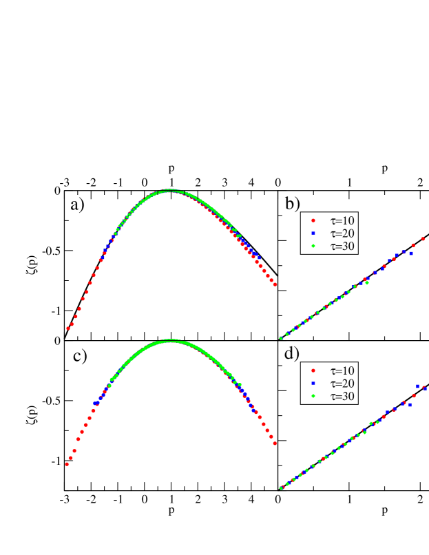
Figure 1: pdf of $\sigma^{diss}_{t}$: a) The large deviation function for the harmonic potential at ${\tau}=10,20,30$; the full line is the analytical result. b) The function $f(p)\equiv[\zeta_{diss}(p)-\zeta_{diss}(-p)]/\sigma^{diss}_{+}$ for the harmonic potential: the fluctuation theorem predicts a straight line with slope 1, represented by a full line. c) The large deviation function for the quartic potential at ${\tau}=10,20,30$. d) The function $f(p)$ for the quartic potential: also in this case the fluctuation theorem is well verified.

The data for ${\cal S}^{diss}_{\tau}$ are shown in Fig. 1. The large deviation function $\zeta_{diss}(p)$ is reported in panel a) for the harmonic and in panel c) for the quartic potential. The average $\sigma^{diss}_{+}$ is equal to $0.332$ in the harmonic case and to $0.276$ in the quartic case. The function $\zeta_{diss}(p)$ converges fast to its asymptotic limit ${\tau}\rightarrow\infty$ (note that even the data for $\tau\sim 10$ are in quite good agreement with the analytic prediction for the harmonic case). The fluctuation theorem predicts $f(p)\equiv[\zeta_{diss}(p)-\zeta_{diss}(-p)]/\sigma^{diss}_{+}=p$. The function $f(p)$ is reported in panel b) for the harmonic and in panel d) for the quartic potential. In the harmonic case the numerical data are compatible with the validity of the fluctuation theorem, as predicted analytically. Remarkably, the same happens in the quartic case for which we do not have an analytical prediction.

These results support the conjecture that, if ${\cal S}^{diss}_{\tau}$ and ${\cal S}^{V}_{\tau}$ are uncorrelated, the pdf of ${\cal S}_{\tau}^{diss}$ verifies the fluctuation theorem independently of the form of the potential $V(x,y)$.

IV.2 Approximate entropy production rate

We also investigated numerically the fluctuations of the entropy production ${\cal S}_{\tau}^{\Theta}$ used in some numerical and experimental studies GGK01 ; CGHLP03 ; FM04 ; Ga04 and that we discussed in section III.2.2. For this model it is given by

$$\sigma^{\Theta}_{t}=\frac{W_{t}}{\Theta}=\frac{2\alpha}{\Theta}\text{Im}\dot{z}_{t}\bar{z}_{t}\ .$$ (94)

Rather arbitrarily we set $\Theta=T_{f}$ in the definition of $\sigma^{\Theta}_{t}$. This reflects what is usually done in numerical simulations, where the dissipated power is divided by the “kinetic” temperature, i.e. the temperature of the fast degrees of freedom. Note that the choice $\Theta=T_{f}$ does not affect the function $\zeta_{\Theta}(p)$ since the variable $p$ is normalized [i.e., $\zeta_{\Theta}(p)\equiv\zeta(p)$ does not depend on $\Theta$, see Eq. (1)] but it changes the average $\sigma^{\Theta}_{+}$ that is proportional to $\Theta^{-1}$.

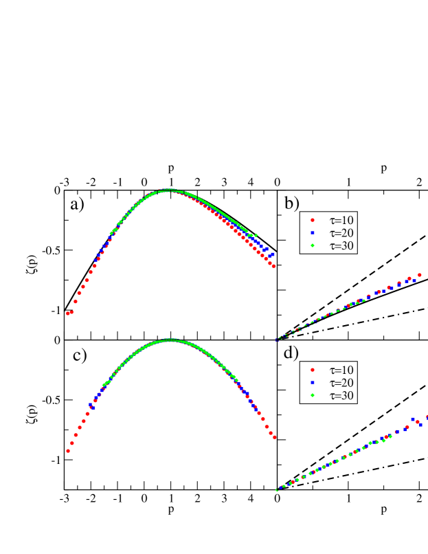
Figure 2: pdf of $\sigma^{\Theta}_{t}$: a) The large deviation function for the harmonic potential at ${\tau}=10,20,30$; the full line is the analytical result. b) The function $f(p)\equiv[\zeta(p)-\zeta(-p)]/\sigma^{T_{f}}_{+}$ for the harmonic potential. The full line is the analytical prediction, the dashed line is the fluctuation relation, the dot-dashed line has slope $T_{f}/T_{s}$. c) The large deviation function for the quartic potential at ${\tau}=10,20,30$. d) The function $f(p)$ for the quartic potential; the dashed line is the fluctuation theorem, the dot-dashed line has slope $T_{f}/T_{s}$.

The data for $\sigma^{\Theta}_{t}$ are reported in Fig. 2. The harmonic case is shown in panels a) and b) while the anharmonic case is presented in panels c) and d). We have $\sigma^{T_{f}}_{+}=0.455$ for the harmonic potential and $\sigma^{T_{f}}_{+}=0.366$ for the quartic one. The numerical result for the large deviation function of $\sigma^{\Theta}_{t}$ agrees very well with the analytical prediction in the harmonic case but, as discussed in section III.2.2, it does not verify the fluctuation theorem for $\Theta=T_{f}$, as one can clearly see from the right panels in Fig. 2.

Remarkably, in both the harmonic and anharmonic cases the function $f(p)\equiv[\zeta(p)-\zeta(-p)]/\sigma^{T_{f}}_{+}$ is approximately linear in $p$ with a slope $X$ such that $1>X>T_{f}/T_{s}$, i.e. $\zeta(p)-\zeta(-p)\sim X\;p\sigma^{T_{f}}_{+}$. If $f(p)\sim Xp$, one can tune the value of $\Theta$ in order to obtain the fluctuation relation $\zeta(p)-\zeta(-p)=p\sigma^{\Theta}_{+}$, by simply choosing $\Theta=\Theta_{eff}=T_{f}/X$, thus defining a single “effective temperature” $\Theta_{eff}\in[T_{f},T_{s}]$. From the data reported in Fig. 2 we get a slope $X\sim 0.66$, that gives $\Theta_{eff}=T_{f}/X\sim 0.9$.

This behavior reflects the one found in some recent experiments ZRA04b ; GGK01 ; CGHLP03 ; FM04 in situations in which the dynamics of the system happens essentially on a single time scale. This is the case also in our numerical simulation: in Fig. 3 we report the autocorrelation function $C(t)=\text{Re}\langle z_{t}\bar{z}_{0}\rangle$ of $z_{t}$ (computed in Appendix D) for the harmonic potential. The present simulation refers to the curve with $\tau_{s}=1$, which clearly decays on a single time scale.

In Fig. 4 we report the parametric plot $\chi(C)$ (see the Introduction and Sect. III) for the same set of parameters, but $\alpha=0$. The integrated response is given by $\chi(t)=\int_{0}^{t}dt^{\prime}\,R(t^{\prime})$ and $R(t)$ is computed in Appendix D. We see that, for $\tau_{s}=1$, the function $\chi(C)$ has a slope close to $-1/T_{f}$ at short times (corresponding to $\chi\sim 0$). For longer times, the slope moves continuously toward $-1/T_{eff}$, with $T_{eff}\sim 1.37$. This value of $T_{eff}$ is of the order of $\frac{\gamma_{f}T_{f}+\gamma_{s}T_{s}}{\gamma_{f}+\gamma_{s}}=1.3$, which means that on time scales of the order of the (unique) relaxation time the two baths behave like a single bath equilibrated at an intermediate temperature. This would be exact if the time scales of the two baths were exactly equal.

It is worth to note that in this situation we get $T_{eff}\neq\Theta_{eff}$, that is, the effective temperature that one would extract from the approximate fluctuation relation of Fig. 2 does not coincide with the effective temperature obtained from the $\chi(C)$ plot of Fig. 4. In particular, we get $T_{f}<\Theta_{eff}<T_{eff}$: this relation is consistent with the results of ZRA04b obtained from the numerical simulation of a sheared Lennard-Jones–like mixture, even if the coincidence might be accidental.

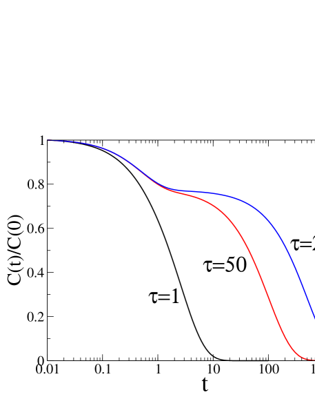
Figure 3: Normalized autocorrelation functions of $z_{t}$ for the harmonic oscillator with $\alpha=0.5$, $k=1$, $T_{f}=0.6$, $T_{s}=2$, $\gamma_{f}=1$, $\gamma_{s}=k\tau_{s}$ and $\tau_{s}=1,50,250$.

IV.3 Discussion

Let us summarize the results in this section. The numerical simulation of the non-linear problem confirms that the fluctuation theorem is satisfied exactly when the entropy production rate $\sigma_{t}^{diss}$ is defined using the power injected by the external drive and the temperature in (18) is used.

In situations in which the dynamics of the system happens on a single time scale, a fitting parameter $\Theta$ can be introduced to obtain an approximate fluctuation relation on the entropy production rate $W_{t}/\Theta$. However, $\Theta$ is not necessarily related to the effective temperature $T_{eff}$ that enters the modified fluctuation–dissipation relation. In the systems considered so far ZRA04b one finds $\Theta<T_{eff}$. However, this is just an approximation that fails in more generic non-equilibrium situations. In the next section we show that, when the dynamics happens on different, well separated, time scales, it is impossible to find a single value of $\Theta$ such that $\sigma^{\Theta}_{t}=W_{t}/\Theta$ verifies the fluctuation relation.

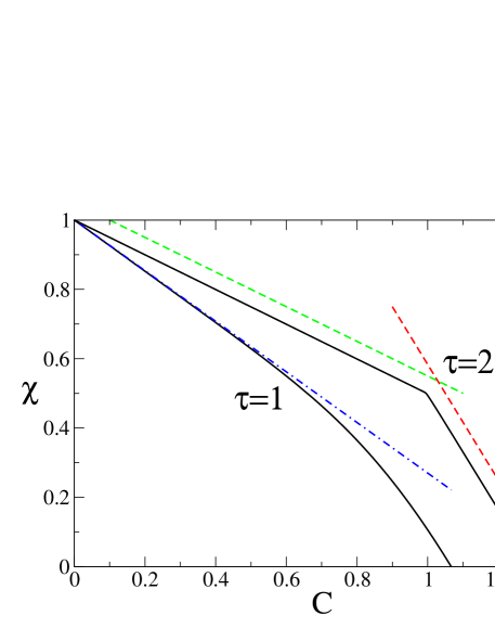
Figure 4: Parametric plot of the integrated response $\chi(t)$ as a function of the correlation function $C(t)$ for the harmonic oscillator with $\alpha=0$, $k=1$, $T_{f}=0.6$, $T_{s}=2$, $\gamma_{f}=1$, $\gamma_{s}=k\tau_{s}$ and $\tau_{s}=1$ (continuous curve) and $\tau_{s}=250$ (broken curve). The dot-dashed line has slope $-1/1.37$, the dashed lines have slope $-1/T_{s}$ and $-1/T_{f}$.

V Separation of time scales and driven glassy systems

In this Section we discuss the application of our results to glassy systems. After presenting the general argument, we show explicitly that the dissipative entropy production satisfies the fluctuation relation for the $p$-spin spherical model. We finally discuss an adiabatic approximation that allows one to derive approximate results in the case of systems with well-separated time-scales.

V.1 Background

As discussed in the Introduction, in the study of mean-field models for glassy dynamics Cu02 ; Cukuja and when using resummation techniques within a perturbative approach to microscopic glassy models with no disorder, effective equations of motion of the form of Eq. (10) are obtained:

$$\gamma\dot{\varphi}_{t}=-\mu(t)\ \varphi_{t}+\int_{-\infty}^{t}dt^{\prime}\ \Sigma(t,t^{\prime})\ \varphi_{t^{\prime}}+\rho_{t}+\alpha h[\varphi_{t}]\ ,$$ (95)

where $\rho_{t}$ is a Gaussian noise such that $\langle\rho_{t}\rho_{t^{\prime}}\rangle=D(t,t^{\prime})$. The “self-energy” $\Sigma(t,t^{\prime})$ and the “vertex” $D(t,t^{\prime})$ depend on the interactions in the system throught the correlation and response of the field $\varphi$. In absence of drive ($\alpha=0$) this equation has a dynamic transition at $T_{d}$ separating a high temperature phase in which the dynamics rapidly equilibrates from a low temperature phase in which the dynamics is non–stationary and the fluctuation–dissipation relation is violated. This means that the time needed for the system to equilibrate is the longest time scale that is unreachable in the calculation (it already diverged with $N$).

In the case of a driven mean field system Cukulepe ; Cukulepe1 ; BBK00 , the external force is also present in Eq. (95) and after a transient the system becomes stationary for any temperature, i.e. $\mu(t)\equiv\mu$, $\Sigma(t,t^{\prime})=\Sigma(t-t^{\prime})$, and $D(t,t^{\prime})=D(t-t^{\prime})$. The functions $D$ and $\Sigma$ depend on the strength $\alpha$ of the driving force. In this case, Eq. (95) resembles Eqs. (78) and (87), and our results of Sect. III apply. By analogy with Eq. (18), the effective temperature is defined in terms of $\Sigma$ and $D$, see below.

As discussed in Cukulepe ; Cukulepe1 ; BBK00 ; BB00 ; BB02 , for small $\alpha$ the system shows a completely different behavior above and below $T_{d}$, reflecting the presence of a dynamical transition at $\alpha=0$. Above $T_{d}$, the fluctuation-dissipation theorem holds in the limit of $\alpha\rightarrow 0$; the transport coefficient related to the driving force $\alpha$ approaches a constant value for $\alpha\rightarrow 0$ (the linear response holds close to equilibrium) and the systems behaves like a “Newtonian fluid”. Below $T_{d}$, the fluctuation-dissipation relation is violated also in the limit $\alpha\rightarrow 0$ and the transport coefficient diverges in this limit: the system is strongly nonlinear. For a wide class of systems, see the Introduction and Ref. Cu02 , the relation between $D$ and $\Sigma$ takes a very simple form in the limit $\alpha\rightarrow 0$: the effective temperature $T_{eff}(t-t^{\prime})$ defined from the ratio between induced integrated response and correlation (see the Introduction) is given by the temperature of the bath $T$ for small $|\,t-t^{\prime}\,|$ and by a constant $T_{eff}>T$ for large $|\,t-t^{\prime}\,|$. Thus, we expect that above $T_{d}$ (and for $\alpha\sim 0$) the system behaves as if coupled to a single equilibrium bath (and the fluctuation theorem holds for the entropy production rate defined as $\sigma_{t}=\alpha h[\varphi_{t}]\dot{\varphi}_{t}/T$), while below $T_{d}$ the system behaves as if coupled to two baths acting on different time scales and equilibrated at different temperatures.

As already remarked in the introduction, these single-spin equations of motion are valid for times $\tau$ that are finite with respect to the size $N$. For these times the system behaves like independent spins moving in a harmonic potential in contact with a nonequilibrium environment. Thus, for ${\cal{S}}_{\tau}$ with $\tau$ in this regime the results of section III apply and the correct definition of the entropy production rate is given by Eq. (80), i.e. by the power injected by the external force alone, divided by the frequency-dependent effective temperature.

V.2 The spherical $p$-spin

The (modified) fluctuation relation can be checked explicitly for the $p$-spin spherical model. This model realizes explicitly the behaviour described above. The asymptotic dynamics in the low temperature phase occurs in a region of phase space that is called the threshold and it is far from the equilibrium states Cuku93 since times that grow with $N$ are needed to reach them.

The effective equations of motion for the driven spherical $p$-spin Cukulepe ; BBK00 are

$$\begin{split}&\partial_{t}C(t,t^{\prime})=-\mu(t)C(t,t^{\prime})+\int dt^{\prime\prime}\Sigma(t,t^{\prime\prime})C(t^{\prime\prime},t^{\prime})+\int dt^{\prime\prime}D(t,t^{\prime\prime})R(t^{\prime},t^{\prime\prime})\ ,\\ &\partial_{t}R(t,t^{\prime})=-\mu(t)R(t,t^{\prime})+\int dt^{\prime\prime}\Sigma(t,t^{\prime\prime})R(t^{\prime\prime},t^{\prime})+\delta(t-t^{\prime})\ ,\\ &\mu(t)=T+\int dt^{\prime}\big{[}D(t,t^{\prime})R(t,t^{\prime})+\Sigma(t,t^{\prime})C(t,t^{\prime})\big{]}\ ,\\ \end{split}$$ (96)

with the vertex and self-energy

$$\begin{split}&D=\frac{p}{2}C^{p-1}+\alpha^{2}\frac{k}{2}C^{k-1}\equiv D_{0}+\alpha^{2}D_{1}\ ,\\ &\Sigma=\frac{1}{2}p(p-1)RC^{p-2}=RD^{\prime}_{0}(C)\ ,\end{split}$$ (97)

respectively. The dynamics can also be described with a “single-spin” Langevin equation of the form

$$\begin{split}&\dot{\varphi}(t)=-\mu(t)\varphi(t)+\int dt^{\prime}\;\Sigma(t,t^{\prime})\varphi(t^{\prime})+\rho(t)\ ,\\ &\langle\rho(t)\rho(t^{\prime})\rangle=2T\delta(t-t^{\prime})+D(t,t^{\prime})\ .\end{split}$$ (98)

Note that $\Sigma$ and $D_{0}$ verify the detailed balance condition. From the expressions (97), one can rewrite Eq. (98), in the stationary case, in the following way

$$\begin{split}&\dot{\varphi}(t)=-\mu\varphi(t)+\int_{-\infty}^{\infty}dt^{\prime}\;\Sigma(t-t^{\prime})\varphi(t^{\prime})+\rho(t)+\alpha h(t)\ ,\\ &\langle\rho(t)\rho(t^{\prime})\rangle=2T\delta(t-t^{\prime})+D_{0}(t-t^{\prime})\ ,\\ &\langle h(t)h(t^{\prime})\rangle=D_{1}(t-t^{\prime})\ ,\end{split}$$ (99)

where $\rho(t)$ and $h(t)$ are two uncorrelated Gaussian variables. Note that $\Sigma$ and $D_{0}$ still depend implicitly on $\alpha$ as one has to solve the self-consistency equations (96) for $C$ and $R$ and substitute the result in $\Sigma$ and $D_{0}$.

In the absence of drive and interpreting $\Sigma$ and $D$ as the response and correlation of a bath, its frequency-dependent effective temperature is

$$T(\omega)=\frac{\nu(\omega)}{2\text{Re}g(\omega)}=\frac{2T+D_{0}(\omega)}{2\text{Re}[1+\Sigma(\omega)/(i\omega)]}\ .$$ (100)

Given that $\Sigma$ and $D$ depend on $R$ and $C$, if one finds that $R$ and $C$ are related by the fluctuation dissipation theorem, $R(t)=-\beta\theta(t)\dot{C}(t)$, from the relation $\Sigma=RD_{0}^{\prime}(C)$ it follows that $T(\omega)\equiv T$ and the bath is in equilibrium, as expected. If $R$ and $C$ do not verify the fluctuation dissipation theorem, $T(\omega)\neq T$.

Switching on the external drive one can compute its dissipated power

$$W(t)=\alpha h(t)\dot{\varphi}(t)\;$$ (101)

and its average. One finds

$$\langle W(t)\rangle = \alpha\langle h(t)\dot{\varphi}(t)\rangle=\alpha\langle h(t)\int_{-\infty}^{\infty}dt^{\prime}\,\dot{R}(t-t^{\prime})\big{[}\rho(t^{\prime})+\alpha h(t^{\prime})\big{]}\rangle$$ (102)

$$= \langle W\rangle=\alpha^{2}\int_{0}^{\infty}dt\,\dot{R}(t)D_{1}(t)=\alpha^{2}\frac{k}{2}\int_{0}^{\infty}dt\,\dot{R}(t)C^{k-1}(t)\ ,$$

consistently with the result of BBK00 where the average of the injected power was explicitly computed for this model. One can prove that the entropy production ${\cal S}^{diss}_{\tau}$ obtained from the rate

$$\sigma_{t}^{diss}=\alpha\int_{-\infty}^{t}dt^{\prime}\,T^{-1}(t-t^{\prime})\big{[}h(t)\dot{\varphi}(t^{\prime})+h(t^{\prime})\dot{\varphi}(t)\big{]}\ ,$$ (103)

verifies the fluctuation relation. Indeed, first rewriting the dissipative entropy production as

$${\cal S}^{diss}_{\tau}=\alpha\frac{\Delta\omega}{2\pi}\sum_{n=-\infty}^{\infty}\frac{h_{n}i\omega_{n}\bar{\varphi}_{n}}{T(\omega_{n})}\ ,$$ (104)

and using the solution for $\varphi_{n}$, in the generic notation of the previous section, one finds

$$\phi_{diss}(\lambda)=\frac{1}{2}\int_{-\infty}^{\infty}\frac{d\omega}{2\pi}\ln\left[1+4\alpha^{2}\lambda(1-\lambda)\frac{\mu(\omega)\omega^{2}[\text{Re}g(\omega)]^{2}}{\nu(\omega)|D(\omega)|^{2}}\right]\ ,$$ (105)

where $\nu$, $\mu$ and $g$ are the Fourier transforms of the $\rho-\rho$ correlator, the $h-h$ correlator and the time-integrated $\Sigma$, respectively. It is easy to check that $\phi_{diss}(\lambda)=\phi_{diss}(1-\lambda)$ and the fluctuation relation is then verified.

Once again, we showed that the dissipative contribution to the entropy production satisfies the fluctuation relation with a modified temperature. Note however that this solvable example is non-trivial for at least two reasons. It is a clearly an-harmonic problem since $\Sigma$ and $D$ are themselves functions of $C$ and $R$. The single spin $\varphi$ is coupled to an equilibrated bath at temperature $T$ and a self-generated “bath” at a different temperature. The temperature entering the fluctuation relation involves both, through the definition (100). This temperature is the one that one would observe by measuring the fluctuation-dissipation relation on the variable $\varphi$.

V.3 The adiabatic approximation

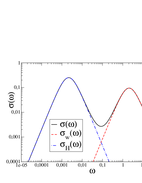
Figure 5: Power spectrum of the entropy production rate (full line) as a function of the frequency for the harmonic oscillator with $\alpha=0.5$, $k=1$, $T_{f}=0.6$, $T_{s}=2$, $\gamma_{f}=1$, $\gamma_{s}=k\tau_{s}$ and $\tau_{s}=250$. The dot-dashed line is the “slow” contribution of $H_{t}$, the dashed line is the “fast” contribution of $w_{t}$.

When a simple system is coupled to a complex bath with two (or more) time scales these are induced into the dynamics of the system. When the time-scales are well separated, an adiabatic treatment is possible in which one separates the dynamic variables in terms that evolve in different time-scales (dictated by the baths) and are otherwise approximately constant.

In this subsection we use an adiabatic approach Cukuja to treat simple problems coupled to baths that evolve on different scales. The motivation for studying this type of problems is that they resemble glassy systems although in the latter the separation of time-scales is self-generated.

We study the pdf of ${\cal S}^{diss}_{\tau}$ and ${\cal S}_{\tau}$. The former satisfies the fluctuation theorem (at least in the harmonic case since corrections due to ${\cal S}^{V}_{\tau}$ might appear in non-harmonic problems). We check that the adiabatic approximation does not spoil this feature. The latter, instead, does not satisfy the fluctuation theorem in general. However, it is interesting to understand under which conditions it satisfies the fluctuation theorem approximately. Indeed, in numerical simulations and experiments it has been customary to measure the dissipated power $W_{t}=\alpha h[\varphi_{t}]\dot{\varphi}_{t}$ and then define the entropy production rate as $\sigma_{t}=W_{t}/T$ (where $T$ is the temperature of the fast bath). This corresponds to the definition of $\sigma^{\Theta}_{t}$, given in Eq. (85) for the harmonic oscillator. We show that when the particle is coupled to a bath that evolves in well-separated time-scales $\sigma^{\Theta}_{t}$ does not satisfy the fluctuation theorem.

V.3.1 The harmonic model coupled to two baths

Let us consider again the Langevin equation (87) with ${\cal V}(|z|^{2})=k|z|^{2}$. In this case, the correlation functions can be calculated explicitly, see Appendix D. In Fig. 3 we report the autocorrelation functions, $C(t)=\langle z_{t}\bar{z}_{0}\rangle$, for $\alpha=0.5$, $k=1$, $T_{f}=0.6$, $T_{s}=2$, $\gamma_{f}=1$, $\gamma_{s}=k\tau_{s}$ and different values of $\tau_{s}$. Clearly, for $k\tau_{s}=\gamma_{s}\gg\gamma_{f}$ two very different time scales –related to the time scales of the two baths– are present. From the plot of Fig. 4 one sees that in the case $k\tau_{s}=250\gg\gamma_{f}$ the function $\chi(C)$ is a broken line with slope $-1/T_{f}$ at large $C$ (short times) and $-1/T_{s}$ for small $C$ (large times).

We want to show that, in this situation, the variable $z_{t}$ can be written as the sum of two quasi-independent contributions. Using the construction introduced in Cukuja we rewrite the equation of motion (87) as

$$\left\{\begin{array}[]{l}\gamma_{f}\dot{z}_{t}=-(k+\gamma_{s}/\tau_{s})z_{t}+i\alpha z_{t}+\rho^{f}_{t}+h_{t}\;,\\ h_{t}=-\frac{\gamma_{s}}{(\tau_{s})^{2}}\int_{-\infty}^{t}dt^{\prime}\ e^{-\frac{t-t^{\prime}}{\tau_{s}}}z_{t^{\prime}}+\rho^{s}_{t}\;.\end{array}\right.$$ (108)

The variable $h_{t}$ is “slow”; if we consider it as a constant in the first equation, the variable $z_{t}$ will fluctuate around the equilibrium position $z_{h}=h/(k+\gamma_{s}/\tau_{s}-i\alpha)\equiv H$. The latter will –slowly– evolve according to the second equation in (108), in which we can approximate $z_{t^{\prime}}\sim H_{t^{\prime}}$. Defining the –fast– displacement of $z_{t}$ with respect to $H_{t}$, $w_{t}\equiv z_{t}-H_{t}$, we obtain the following equations for $(w_{t},H_{t})$:

$$\begin{cases}&\gamma_{f}\dot{w}_{t}=-(k+\gamma_{s}/\tau_{s})w_{t}+i\alpha w_{t}+\rho^{f}_{t}\ ,\\ &\frac{\gamma_{s}}{\tau_{s}}\int_{-\infty}^{t}dt^{\prime}\ e^{-\frac{t-t^{\prime}}{\tau_{s}}}\dot{H}_{t^{\prime}}=-kH_{t}+i\alpha H_{t}+\rho^{s}_{t}\ .\end{cases}$$ (109)

In this approximation, $z_{t}=H_{t}+w_{t}$ is the sum of two contributions: $w_{t}$ is a “fast” variable which evolves according to a Langevin equation with the fast bath only and a renormalized harmonic constant $k+\gamma_{s}/\tau_{s}$, while $H_{t}$ is a “slow” variable which evolves according to a Langevin equation where the slow bath only appears. In both equations the driving force $\alpha$ is present, thus we expect both $H_{t}$ and $w_{t}$ to contribute to the dissipation. Note that $w_{t}$ and $H_{t}$ are completely uncorrelated in this approximation.

V.3.2 The “potential” entropy production rate $\sigma^{V}_{t}$

In the adiabatic approximation the term ${\cal{S}}^{V}_{\tau}$ in equation (41) should become a boundary term. Indeed, the function $T^{-1}(t)$, in the adiabatic approximation, becomes

$$T^{-1}(t)=\frac{1}{T_{f}}\delta(t)+T^{-1}_{s}(t)\ ,$$ (110)

where the function $T_{s}^{-1}(t)$ is “slow”, see e.g. Eq. (93). Inserting this expression in $\sigma^{V}_{t}$, the first term gives a total derivative. The second term gives

$$\int_{-\infty}^{t}dt^{\prime}\,T^{-1}_{s}(t-t^{\prime})\left[\dot{r}_{\alpha}(t)\frac{\partial V}{\partial r_{\alpha}}[\vec{r}(t^{\prime})]+\dot{r}_{\alpha}(t^{\prime})\frac{\partial V}{\partial r_{\alpha}}[\vec{r}(t)]\right]\ .$$ (111)

Due to the convolution with the “slow” function $T^{-1}_{s}(t)$, the fast components of $r$ are irrelevant in the integral, while for the slow ones it is reasonable to replace $\dot{r}_{\alpha}(t)$ with $\dot{r}_{\alpha}(t^{\prime})$ on the scale $\tau_{s}$ over which $T^{-1}_{s}(t)$ decays. Thus one obtains a total derivative times the integral of $T^{-1}_{s}(t)$ which is a finite constant. Obviously this is not a rigorous proof and should be checked numerically in concrete cases.

V.3.3 The “dissipative” entropy production rate $\sigma^{diss}_{t}$

The entropy production rate defined in Eqs. (80) and (91) can be rewritten in terms of $H_{t}$ and $w_{t}$. Recalling that $T^{-1}(t)$ is defined by Eq. (93) one obtains (the details of the calculation are reported in Appendix E)

$$\sigma^{diss}_{t}\sim 2\alpha\text{Im}\left[\frac{\dot{w}_{t}\bar{w}_{t}}{T_{f}}+\frac{\dot{H}_{t}\bar{H}_{t}}{T_{s}}\right]$$ (112)

neglecting terms that vanish when $\sigma^{diss}_{t}$ is integrated over time intervals of the order of $\tau_{s}$. This is exactly the entropy production expected for two independent systems.

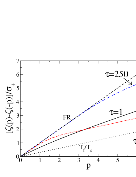
Figure 6: The function $[\zeta_{\Theta}(p)-\zeta_{\Theta}(-p)]/\sigma^{\Theta}_{+}$ for the harmonic oscillator with $\alpha=0.5$, $k=1$, $\Theta=T_{f}=0.6$, $T_{s}=2$, $\gamma_{f}=1$, $\gamma_{s}=k\tau_{s}$ and $\tau_{s}=1,50,250$. The dashed line (FR) is a straight line with slope 1, the dotted line has slope $T_{f}/T_{s}=0.3$.

To check that this approximation works well, let us introduce a “power spectrum” $\sigma(\omega)d\omega$ as the contribution coming from frequencies $[\omega,\omega+d\omega]$ to the average entropy production rate, $\sigma^{diss}_{+}=\int_{0}^{\infty}d\omega\,\sigma(\omega)$. From Eq. (84) we get

$$\begin{split}&\sigma^{diss}_{+}=\left.\frac{d\phi_{diss}}{d\lambda}\right|_{\lambda=0}=-\int_{-\infty}^{\infty}\frac{d\omega}{2\pi}\frac{2\alpha\omega\nu(\omega)}{|D(\omega)|^{2}}\\ &\sigma(\omega)=\frac{1}{2\pi}\left[-\frac{2\alpha\omega\nu(\omega)}{|D(\omega)|^{2}}+\frac{2\alpha\omega\nu(-\omega)}{|D(-\omega)|^{2}}\right]=\frac{\alpha\omega\nu(\omega)}{\pi}\left[\frac{1}{|D(-\omega)|^{2}}-\frac{1}{|D(\omega)|^{2}}\right]\end{split}$$ (113)

Substituting the expressions of $\nu(\omega)$ and of $D(\omega)$ appropriate for Eq. (87) we get the power spectrum $\sigma(\omega)$ as a function of $\omega$ which is reported in Fig. 5 as a full line. The contributions of $w_{t}$ and $H_{t}$, $\sigma_{w}(\omega)$ and $\sigma_{H}(\omega)$, are obtained inserting in Eq. (113) the expression of $\nu(\omega)$ and $D(\omega)$ obtained from the two equations (109). They are reported as dashed and dot-dashed lines in Fig. 5. We can conclude that, for $k\tau_{s}\gg\gamma_{f}$, the adiabatic approximation holds and $\sigma^{diss}_{t}=\sigma^{w}_{t}+\sigma^{H}_{t}$, with $\sigma^{w}_{t}=2\alpha\text{Im}\,\dot{w}_{t}\bar{w}_{t}/T_{f}$ and $\sigma^{H}_{t}=2\alpha\text{Im}\,\dot{H}_{t}\bar{H}_{t}/T_{s}$, and the two contributions are independent. Note that the average dissipation due to $H$ is much larger than the one due to $w$. Finally, we can write:

$$\phi_{diss}(\lambda)=\phi^{w}(\lambda)+\phi^{H}(\lambda)\ ,\hskip 30.0pt\phi^{w,H}(\lambda)=-\lim_{\tau\rightarrow\infty}\tau^{-1}\ln\langle\exp\big{[}-\lambda\sigma^{w,H}\big{]}\rangle\ .$$ (114)

Both $\phi^{w}(\lambda)$ and $\phi^{H}(\lambda)$ verify the fluctuation theorem, as the two equations of motion (109) are particular instances of the general case discussed in section III. The function $\zeta_{diss}(p)$ is the Legendre transform of $\phi_{diss}(\lambda)$ and will verify the fluctuation theorem.

V.3.4 The “approximate” entropy production rate $\sigma^{\Theta}_{t}$

In the same approximation, $\sigma^{\Theta}_{t}$ is given, for $\Theta=T_{f}$, by

$$\sigma^{T_{f}}_{t}=2\alpha\text{Im}\left[\frac{\dot{w}_{t}\bar{w}_{t}+\dot{H}_{t}\bar{H}_{t}}{T_{f}}\right]=\sigma^{w}_{t}+\frac{T_{s}}{T_{f}}\sigma^{H}_{t}\ ,\hskip 20.0pt\text{and}\hskip 20.0pt\phi_{T_{f}}(\lambda)=\phi^{w}(\lambda)+\phi^{H}(\lambda T_{s}/T_{f})\ ;$$ (115)

the contribution of $H_{t}$ is weighted with the “wrong” temperature, i.e. the temperature of the fast degrees of freedom. Indeed, as we have already discussed, $\phi_{\Theta}(\lambda)$ does not verify the fluctuation theorem. The function $f(p)\equiv[\zeta_{\Theta}(p)-\zeta_{\Theta}(-p)]/\sigma^{\Theta}_{+}$ [obtained from Eq. (86)] is reported in Fig. 6. As already discussed in section IV, when the time scales of the two baths are of the same order, $k\tau_{s}\sim\gamma_{f}$, the two baths act like a single bath at temperature $\Theta\in[T_{f},T_{s}]$ and the function $f(p)$ is approximately linear in $p$ with slope $X\in[T_{f}/T_{s},1]$. When the time scales are well separated, $k\tau_{s}\gg\gamma_{f}$, the adiabatic approximation holds; and one finds that $f(p)$ has slope $\sim 1$ for small $p$ and $T_{f}/T_{s}$ for large $p$ (see Fig. 6).

The results for $k\tau_{s}\sim\gamma_{f}$ are consistent with the ones in ZRA04b where only the situation in which the two time scales are not well separated could be investigated. Indeed, when the dynamics becomes very slow the observation of large negative fluctuations of the entropy production requires a huge amount of computational time and the function $f(p)$ can be calculated only in a narrow range of $p$ around $p=0$. Note that the value of $p$ at which the slope of $f(p)$ crosses over from $1$ to $T_{f}/T_{s}$ depend on the values of the parameters $\alpha$, $\gamma_{f}$, $\gamma_{s}$, $\tau_{s}$, etc. and can be of the order of $5$, while in numerical simulations one can usually reach values of – at most – $p\sim 3$. Thus, the observation of curves like the one reported in Fig. 6 in numerical simulations of glassy systems is a very difficult task.

VI Green-Kubo relations

It was proven in Ga96a ; Ga96b that the fluctuation theorem implies, in the equilibrium limit ($\sigma_{+}\rightarrow 0$) the Green-Kubo relation for transport coefficients. This is a particular form of the fluctuation–dissipation theorem. In this Section we discuss how one links the modified fluctuation theorem – in which we replaced the external bath temperature by the (frequency dependent) effective temperature of the unperturbed system – to the modification of the fluctuation dissipation relation.

VI.1 General derivation

Let us recall briefly how the Green-Kubo relation can be obtained from the fluctuation theorem. Suppose that we apply a (constant) driving force $E$ to a system in equilibrium. This generates a corresponding flux $J_{t}$ (e.g. if $E$ is an electric field $J_{t}$ is the electric current) such that, close to equilibrium, the dissipated power can be written as $W_{t}=EJ_{t}$. The entropy production rate is then

$$\sigma_{t}=\frac{W_{t}}{T}=\frac{EJ_{t}}{T}\ .$$ (116)

The fluctuation theorem can be written as $\phi(\lambda)=\phi(1-\lambda)$ where $\phi(\lambda)$ is defined in Eq. (25). The derivatives of $\phi(\lambda)$ are the moments of ${\cal S}_{\tau}$, i.e.

$$\phi_{k}\equiv\left.\frac{d^{k}\phi}{d\lambda^{k}}\right|_{\lambda=0}=(-1)^{k-1}\lim_{\tau\rightarrow\infty}\tau^{-1}\langle{\cal S}_{\tau}^{k}\rangle_{c}\ ,$$ (117)

where $\langle A^{2}\rangle_{c}=\langle A^{2}\rangle-\langle A\rangle^{2}$ and so on. Thus, $\phi_{k}\sim\sigma_{+}^{k}$, and close to equilibrium ($\sigma_{+}\sim 0$) $\phi(\lambda)$ is well approximated by a second order polynomial (corresponding to a Gaussian pdf),

$$\phi(\lambda)\sim\phi_{0}+\phi_{1}\lambda+\frac{\phi_{2}}{2}\lambda^{2}\ .$$ (118)

Then the fluctuation relation, $\phi(\lambda)=\phi(1-\lambda)$, implies $\phi_{2}=-2\phi_{1}$; from Eq. (117) and using time-translation invariance,

$$\phi_{2}=-2\phi_{1}\hskip 10.0pt\Rightarrow\hskip 10.0pt\sigma_{+}=\int_{0}^{\infty}dt\ \langle\sigma_{t}\sigma_{0}\rangle_{c}\ .$$ (119)

Substituting $\sigma_{t}=EJ_{t}/T$ one obtains

$$\langle J\rangle_{E}=\frac{E}{T}\int_{0}^{\infty}dt\ \langle J_{t}J_{0}\rangle_{E=0}+o(E^{2})\ ,$$ (120)

that is to say, the Green-Kubo relation.

Note that even out of equilibrium one can define a flux ${\cal J}_{t}$ using $\sigma_{t}$ as a “Lagrangian”, see Ref. Ga04 :

$${\cal J}_{t}=\frac{\partial\sigma_{t}}{\partial E}\ .$$ (121)

Close to equilibrium $\sigma_{t}$ is given by Eq. (116) and ${\cal J}_{t}=J_{t}/T$. If, in the absence of a drive, the system has a non trivial effective temperature, the entropy production rate should be defined as in Eqs. (80) and (91). Then the flux ${\cal J}_{t}$ is given by

$${\cal J}_{t}=\frac{\partial\sigma^{diss}_{t}}{\partial\alpha}=4\,\text{Im}\int_{-\infty}^{t}dt^{\prime}T^{-1}(t-t^{\prime})\dot{z}_{t}\bar{z}_{t^{\prime}}=2\int_{-\infty}^{t}dt^{\prime}T^{-1}(t-t^{\prime})[\dot{y}_{t}x_{t^{\prime}}-\dot{x}_{t}y_{t^{\prime}}]\ .$$ (122)

The fluctuation theorem for $\sigma^{diss}$ implies then a Green-Kubo relation for ${\cal J}_{t}$:

$$\langle{\cal J}\rangle_{\alpha}=\alpha\int_{0}^{\infty}dt\ \langle{\cal J}_{t}{\cal J}_{0}\rangle_{\alpha=0}+o(\alpha^{2})\ .$$ (123)

The physical meaning of the latter relation becomes clear if one writes the flux ${\cal J}_{t}$ in the adiabatic approximation discussed in the previous section; from Eq. (112)

$${\cal J}_{t}=2\text{Im}\left[\frac{\dot{w}_{t}\bar{w}_{t}}{T_{f}}+\frac{\dot{H}_{t}\bar{H}_{t}}{T_{s}}\right]=\frac{J^{w}_{t}}{T_{f}}+\frac{J^{H}_{t}}{T_{s}}\ ,$$ (124)

and Eq. (123) becomes

$$\frac{\langle J^{w}\rangle_{\alpha}}{T_{f}}+\frac{\langle J^{H}\rangle_{\alpha}}{T_{s}}=\frac{\alpha}{T_{f}^{2}}\int_{0}^{\infty}dt\ \langle J^{w}_{t}J^{w}_{0}\rangle_{\alpha=0}+\frac{\alpha}{T_{s}^{2}}\int_{0}^{\infty}dt\ \langle J^{H}_{t}J^{H}_{0}\rangle_{\alpha=0}+o(\alpha^{2})\ .$$ (125)

Indeed, in the adiabatic approximation the Green-Kubo relation holds separately for $J^{w}_{t}$ (with temperature $T_{f}$) and for $J^{H}_{t}$ (with temperature $T_{s}$). Eq. (123) encodes the two contributions and holds even when the adiabatic approximation does not apply and the contributions of the “fast” and of the “slow” modes is not well separated.

Note that the “classical” Green-Kubo relation involves the total flux $J_{t}=J^{w}_{t}+J^{H}_{t}$. For the latter one has, in the adiabatic approximation,

$$\begin{split}\langle J_{t}\rangle_{\alpha}&=\langle J^{w}_{t}\rangle_{\alpha}+\langle J^{H}_{t}\rangle_{\alpha}=\frac{\alpha}{T_{f}}\int_{0}^{\infty}dt\ \langle J^{w}_{t}J^{w}_{0}\rangle_{\alpha=0}+\frac{\alpha}{T_{s}}\int_{0}^{\infty}dt\ \langle J^{H}_{t}J^{H}_{0}\rangle_{\alpha=0}\\ &=\alpha\int_{0}^{\infty}dt\left[\frac{\langle J^{w}_{t}J^{w}_{0}\rangle_{\alpha=0}}{T_{f}}+\frac{\langle J^{H}_{t}J^{H}_{0}\rangle_{\alpha=0}}{T_{s}}\right]\sim\alpha\int_{0}^{\infty}dt\frac{1}{T_{eff}(t)}\langle J_{t}J_{0}\rangle_{\alpha=0}\ .\end{split}$$ (126)

The latter relation is the generalization of the Green-Kubo formula that comes from the generalized fluctuation-dissipation relation discussed in the Introduction and Section III. It is closely related, but not equivalent, to Eq. (123).

VI.2 The Green-Kubo relation for driven glassy systems

Eqs. (123) and (126) cannot be applied straightforwardly to driven glassy systems as for these systems the correlation function $\langle J_{t}J_{0}\rangle_{\alpha}$ is not stationary at $\alpha=0$ at low temperatures. Indeed, the relaxation time of the latter grows very fast as $\alpha\rightarrow 0$ and at some point falls outside the experimentally accessible range: the system will not be able to reach stationarity on the experimental time scales and will start to age indefinitely.

However, let us consider again the equation of motion (10) for $\alpha\neq 0$, where we assume that a stationary state is reached,

$$\gamma\dot{\varphi}_{t}=-\mu_{\alpha}\ \varphi_{t}+\int_{-\infty}^{t}dt^{\prime}\ \Sigma_{\alpha}(t-t^{\prime})\ \varphi_{t^{\prime}}+\rho_{t}+\alpha h[\varphi_{t}]\ ,\hskip 20.0pt\langle\rho_{t}\rho_{t^{\prime}}\rangle=D_{\alpha}(t-t^{\prime})\ .$$ (127)

The functions $\Sigma_{\alpha}(t-t^{\prime})$ and $D_{\alpha}(t-t^{\prime})$ depend (strongly) on $\alpha$; indeed, as the term explicitly proportional to $\alpha$ is a small perturbation for $\alpha\sim 0$, the main contribution to the $\alpha$-dependence of the dynamics of $\varphi_{t}$ will come from the $\alpha$-dependence of $\Sigma_{\alpha}$ and $D_{\alpha}$. If we compare the latter equation with Eq. (87), we see that setting $\alpha=0$ in Eq. (87) is equivalent to setting $\alpha=0$ without changing the functions $\Sigma$ and $D$ in Eq. (127). This will not affect too much the correlation function $\langle J_{t}J_{0}\rangle_{\alpha}$ if $\alpha$ is small. Finally, we can write, for small $\alpha$,

$$\langle J_{t}\rangle_{\alpha}\sim\alpha\int_{0}^{\infty}dt\frac{1}{T_{eff}(t)}\langle J_{t}J_{0}\rangle_{\alpha}\ ,$$ (128)

even if the limit $\alpha\rightarrow 0$ is not well defined. An analogous relation will be obtained from Eq. (123) (which is equivalent to the fluctuation theorem in the Gaussian approximation) within the same approximation. The latter relations can be tested in numerical simulations as well as in experiments.

VII Slow periodic drive and effective temperature

In this Section we discuss a means to measure an effective temperature associated to slow timescales of a non-equilibrium system by using the modification of the fluctuation theorem.

A lesson we learn from the previous calculations (see e.g. Fig. 5) is that the work done at large frequencies is overwhelmingly larger than that done at very low frequencies – precisely the one we wish to observe in order to detect effective temperatures. One way out of this is to choose a perturbation that does little work at high frequencies: a periodically time-dependent force that derives from a potential $\cos(\Omega t){\tilde{V}}(r)$, with $1/\Omega$ of the order of timescale of the slow bath $\tau_{s}$. Let us show this for a one dimensional system, the generalization being straightforward.

VII.1 General derivation

Let us consider a single degree of freedom $r$ moving in a time-independent potential $V(r)$ and subject to a periodically time-dependent field $\cos(\Omega t){\tilde{V}}(r)$, and in contact with a ‘fast’ and a ‘slow’ bath with friction kernel, thermal noise and temperature $(\rho^{f},g_{f},T_{f})$ and $(\rho^{s},g_{s},T_{s})$, respectively:

$$m\ddot{r}(t)+\int_{-\infty}^{t}dt^{\prime}\;g_{f}(t-t^{\prime}){\dot{r}}(t^{\prime})+\int_{-\infty}^{t}dt^{\prime}\;g_{s}(t-t^{\prime}){\dot{r}}(t^{\prime})=-\frac{\partial V}{\partial r}[r(t)]+\rho^{f}(t)+\rho^{s}(t)-\cos(\Omega t)\frac{\partial{\tilde{V}}}{\partial r}[r(t)]\;,$$ (129)

The time scale of the time dependent field $1/\Omega$ is of the same order as the one of the ‘slow’ bath. The work in an interval of time $(0,\tau)$ done by the time-dependent potential is:

$$W_{\tau}=-\int_{0}^{\tau}\;\cos(\Omega t^{\prime})\;\frac{\partial{\tilde{V}}}{\partial r}\;\dot{r}\;dt^{\prime}=-{\tilde{V}}(\tau)+{\tilde{V}}(0)+\Omega\int_{0}^{\tau}\;\sin(\Omega t^{\prime})\;{\tilde{V}}\;dt^{\prime}\ .$$ (130)

Only the last term grows with the number of cycles, so for long times we can neglect the first two. Now, integrating (129) by parts, we obtain

$$m\ddot{r}(t) = -\int_{-\infty}^{t}dt^{\prime}\;g_{f}(t-t^{\prime}){\dot{r}}(t^{\prime})-\frac{\partial V}{\partial r}[r(t)]+\rho^{f}+h(t)-\hat{h}(t)\frac{\partial{\tilde{V}}}{\partial r}[r(t)]$$ (131)

$$h(t) \equiv -\int_{-\infty}^{t}dt^{\prime}\;g_{s}(t-t^{\prime})r(t^{\prime})+\rho^{s}(t)\;.$$ (132)

where $\hat{h}(t)=\cos(\Omega t)$. In the adiabatic limit when both the timescales of the slow bath and the period $1/\Omega$ of the potential $\tilde{V}$ are large, $h(t)$ and $\hat{h}(t)$ are quasi-static. Hence, $r$ has a fast evolution given by Eq. (131) with $h$ and $\hat{h}$ fixed and it reaches a distribution Cukuja

$$P(r/h,\hat{h})=\frac{e^{-\beta_{f}\left(V+\hat{h}{\tilde{V}}+g_{f}(0)\frac{r^{2}}{2}-hr\right)}}{\int\;dr\;e^{-\beta_{f}\left(V+\hat{h}{\tilde{V}}+g_{f}(0)\frac{r^{2}}{2}-hr\right)}}\;.$$ (133)

The denominator defines $Z(h,\hat{h})$ and $F(h,\hat{h})\equiv-\beta_{f}^{-1}\ln Z(h,\hat{h})$. Note that $F(h,\hat{h}(t))$ is periodically time-dependent through $\hat{h}$. The approximate evolution of $h$ is now given by Eq. (132) with the replacement of $r$ in the friction term by its average $\frac{\partial F(h,\hat{h})}{\partial h}$ with respect to the fast evolution:

$$h(t)=\int_{-\infty}^{t}dt^{\prime}\,g_{s}(t-t^{\prime})\frac{\partial F(h,\hat{h})}{\partial h}(t^{\prime})+\rho^{s}(t)\;.$$ (134)

Eq. (134) is in fact a generalized Langevin equation for a system coupled to a (slow) bath of temperature $T_{s}$. Indeed, it can be shown Cukuja to be equivalent to a set of degrees of freedom $y_{i}$ evolving according to the ordinary Langevin equation:

$$\left[m_{j}\frac{d^{2}}{dt^{2}}+\gamma_{j}\frac{d}{dt}+\Omega_{j}\right]y_{j}=\xi_{j}(t)-\frac{\partial F\left(\sum_{j}A_{j}y_{j}\right)}{\partial y_{j}}$$ (135)

with $\langle\xi_{i}(t)\xi_{j}(t^{\prime})\rangle=2T_{s}\gamma_{j}\delta_{ij}\delta(t-t^{\prime})$, provided that the Fourier transforms $g_{s}(\omega)$ an $\nu_{s}(\omega)$ of friction kernel and noise autocorrelation can be written as:

$$g(\omega)=\sum_{j}\frac{A^{2}_{j}}{m_{j}(\omega-\omega_{j}^{+})(\omega-\omega_{j}^{-})}\qquad\qquad\nu(\omega)=2T_{s}\sum_{j}\frac{\gamma_{j}A^{2}_{j}}{m^{2}_{j}(\omega-\omega_{j}^{+})(\omega-\omega_{j}^{-})(\omega+\omega_{j}^{+})(\omega+\omega_{j}^{-})}$$ (136)

where $\omega^{\pm}_{j}$ are the roots of $-m_{j}\omega^{2}+i\gamma_{j}\omega+\Omega_{j}=0$.

Within the same approximation leading to (134), the average of $\tilde{V}(r)$ over a time window $\Delta$ that is long compared to the short timescale, but sufficiently slow that we can consider that $h$ and $\hat{h}$ are constant is

$$\int_{t}^{t+\Delta}\;\tilde{V}(r(t^{\prime}))\;dt^{\prime}\sim\Delta\int\;dr\;P(r/h,\hat{h})\;\tilde{V}(r)=\Delta\frac{\partial F(h,\hat{h})}{\partial\hat{h}}$$ (137)

so that we obtain

$$W_{\tau}\sim\Omega\int_{0}^{\tau}\sin(\Omega t^{\prime})\frac{\partial F(h,\hat{h}(t^{\prime}))}{\partial\hat{h}}dt^{\prime}=-\int_{0}^{\tau}\;\frac{\partial F(h,\hat{h}(t^{\prime}))}{\partial t^{\prime}}dt^{\prime}$$ (138)

which tells us that for long time intervals the work done by the original time-dependent potential $\tilde{V}$ is indeed the same as the work done by the time-dependent effective potential $F$ in (134).

The fluctuation theorem then holds for the distribution of this work, with a single temperature $T_{s}$. We conclude that the distribution of work due to a slow perturbation satisfies the fluctuation theorem with only the slow temperature, and can be hence used experimentally to detect it.

VII.2 Experimental realization

The simplest application of the above general result is obtained considering $\tilde{V}(r)=\tilde{h}r$ and $V(r)=kr^{2}$. Then, grouping together the two noises in a single one with friction $g=g_{f}+g_{s}$ and correlation $\nu=T_{f}\nu_{f}+T_{s}\nu_{s}$ as described in Sect. III, Eq. (129) simply becomes

$$m\ddot{r}(t)+\int_{-\infty}^{t}dt^{\prime}\,g(t-t^{\prime})\dot{r}(t^{\prime})=-kr(t)+\rho(t)+\tilde{h}\cos(\Omega t)\ .$$ (139)

This equation describes for instance the motion of a Brownian particle moving in an out of equilibrium environment and trapped by an harmonic potential whose center oscillates at frequency $\Omega$. A concrete experimental realization of this setting has been already considered in AG04 : Silica beads of $\sim 2\mu$m diameter were dispersed in a solution of Laponite (a particular clay of $\sim 30$nm diameter) and water. The Laponite suspension form a glass for large enough concentration of clay and provides the nonequilibrium environment. The Silica beads are Brownian particles diffusing in such environment. They can be trapped by optical tweezing, and the center of the trap can oscillate with respect to the sample if the latter is oscillated through a piezoelectric stage. In AG04 the mobility and diffusion of tracer particles were measured obtaining an estimate of $T_{eff}(\Omega)$. Here we propose to measure the work done by the trap on the tracers. Indeed, the work dissipated in $(0,\tau)$ is linear in $r(t)$ so it should be possible to measure it simply through the measurement of $r(t)$:

$$W_{\tau}=\Omega\tilde{h}\int_{0}^{\tau}dt^{\prime}\sin(\Omega t^{\prime})r(t^{\prime})\ ;$$ (140)

note that, as $W_{\tau}$ is linear in $r(t)$, it is a Gaussian variable. With a simple calculation one finds

$$\lim_{\tau\rightarrow\infty}\frac{\langle(W_{\tau}-\langle W_{\tau}\rangle)^{2}\rangle}{2\langle W_{\tau}\rangle}=\frac{\nu(\Omega)}{2\text{Re}g(\Omega)}=T_{eff}(\Omega)$$ (141)

This means that the (Gaussian) pdf of ${\cal S}^{diss}_{\tau}=W_{\tau}/T_{eff}(\Omega)$ satisfies the fluctuation relation. If the two baths are modeled as in Sect. IV with $k\gamma_{s}=\tau_{s}\gg\gamma_{f}$ one has $T_{eff}(\Omega)=T_{s}$ for $\Omega\tau_{s}<1$ [see Eq. (92)]. The measurement of the distribution of the work (140) allows for the measurement of $T_{s}$. Note that other experimental settings described by the same equations should exist.

VIII Conclusions

We studied the extension of the fluctuation relation to open stochastic systems that are not able to equilibrate with their environments.

We used the simplest example at hand to test several generalized fluctuation formulas: a Brownian particle in a confining potential coupled to non-trivial external baths with different time-scales and temperatures. Independently of the form of the potential energies, due to the coupling to the complex environment, the particle is not able to equilibrate. Its relaxational dynamics is characterized by an effective temperature, defined via the modification of the fluctuation-dissipation relation between spontaneous and induced fluctuations Cukupe . When no separation of time-scales can be identified in the bath, the effective temperature is a non-trivial function of the two times involved. Instead, when the bath evolves in different time-scales each characterized by a value of a temperature, the two-time dependent effective temperature is a piece-wise function that actually takes only these values, each one characterizing the dynamics of the particle in a regime of times.

Several authors discussed the possibility of introducing the effective temperature in the fluctuation theorem to extend its domain of applicability to glassy models driven by external forces Se98 ; CR04 ; SCM04 ; Sasa . After summarizing our results we shall discuss how they compare to the proposals and findings in these papers.

VIII.1 Summary of results

We here examined carefully different definitions of entropy production rate that are not equivalent when the effective temperature is not trivially equal to the ambient temperature. We found that:

1. The pdf of the “dissipative” entropy production ${\cal S}^{diss}_{\tau}$ that involves the frequency dependent temperature,

   $${\cal{S}}_{\tau}^{diss}=\frac{\Delta\omega}{2\pi}\sum_{n=-\infty}^{\infty}\frac{-i\omega_{n}r_{\alpha}(\omega_{n})h_{\alpha}(\omega_{n})}{T(\omega_{n})}=\int_{-{\tau}/2}^{{\tau}/2}dt\int_{-{\tau}/2}^{{\tau}/2}dt^{\prime}\,T^{-1}(t-t^{\prime})\dot{r}_{\alpha}(t)h_{\alpha}[\vec{r}(t^{\prime})]\ ,$$ (142)

   with $T^{-1}(t)$ the Fourier transform of $1/T(\omega)$, the effective temperature of the relaxing system, see Eq. (18), verifies the fluctuation theorem exactly for harmonic system. It also holds for general systems connected to baths with different temperaures acting on widely separated scales.

2. For nonlinear systems in contact to nonequilibrium baths acting on overlapping timescales an additional term ${\cal S}^{V}_{\tau}$, see Eq. (41), has to be included in the entropy production to make the fluctuation relation hold strictly. Our numerical simulations suggest that, surprisingly enough, the effect of this extra ‘internal’ term is even then quite small.

3. The pdf of ${\cal S}^{\Theta}_{\tau}$ with $\sigma_{t}^{\Theta}=W_{t}/\Theta$, $W_{t}$ the power dissipated by the external force and $\Theta$ a free parameter with the dimensions of a temperature, does not satisfy the fluctuation theorem in general for any choice of $\Theta$.

   The large deviation function, $\zeta_{\Theta}(p)$, still shows some interesting features revealing the existence of an effective temperature. When the bath has, say, two components acting on different time scales and with different temperatures, the function $[\zeta_{\Theta}(p)-\zeta_{\Theta}(-p)]/\sigma^{\Theta}_{+}$ may have different slopes corresponding to these two temperatures, one at small $p$ and the other at large $p$. The separation of time-scales of the bath translates into a separation of scales in the function $[\zeta_{\Theta}(p)-\zeta_{\Theta}(-p)]/\sigma^{\Theta}_{+}$.

   When the time scales of the baths are not separated, and one records the large deviation function for not too large values of $p$ only, the fluctuation theorem is verified approximately if $\Theta$ is suitably chosen. Note that the value of $\Theta$ found in this way is not equal to the effective temperature $T_{eff}$ that enters the modified fluctuation–dissipation relation. Instead, when the time-scales are well separated, the two scales in the large deviation function are clearly visible and a single fitting parameter is not sufficient to make the fluctuation theorem hold.

4. If two time scales are present in the dynamics of a system and the applied perturbation is periodic with frequency $\Omega<1/\tau_{s}$, $\tau_{s}$ being the largest relaxation time, the pdf of the power dissipated over a (large) number of cycles verifies the fluctuation relation with temperature $T_{s}=T_{eff}(\Omega)$. This is probably the easiest way of detecting the effective temperature by means of the fluctuation relation.

These results should apply to driven glassy systems as discussed in section V and are indeed consistent with recent numerical simulations ZRA04b . Models like the one discussed here have been recently investigated Cukuja ; AG04 ; PM04 ; Po04 to describe the dynamics of Brownian particles in complex media such as glasses, granular matter, etc. Brownian particles are often used as probes in order to study the properties of the medium (e.g. in Dynamic Light Scattering or Diffusing Wave Spectroscopy experiments). Moreover, confining potentials for Brownian particles can be generated using laser beams Gr03 and experiments on the fluctuations of the power dissipated in such systems are currently being performed AG04 ; WSMSE02 .

VIII.2 Temperatures

It is important to summarize the different definitions of effective temperature we considered and the relations between them. We defined the effective temperature in the frequency domain in equation (18) as a property of the bath which can also be measured from the ratio between correlation and response functions in the frequency domain. As we discussed above, the same effective temperature enters the correct definition of entropy production rate in the frequency domain, see equation (142). Thus, experiments working in the frequency domain should observe the same effective temperature from the fluctuation–dissipation relation and the fluctuation relation.

In the time domain the situation is slightly more complicated. On the one hand, the effective temperature obtained from the fluctuation–dissipation relation in the time domain, defined for example by Eq. (9), is not the Fourier transform of $T(\omega)$. A convolution with the correlation function is involved in the relation between $T(\omega)$ and $T_{eff}(t)$. On the other hand, the effective temperature $T^{-1}(t)$ entering the entropy production is exactly the Fourier transform of $1/T(\omega)$, see again Eq. (142). This can give rise to ambiguities when working in the time domain.

Most of these ambiguities disappear as long as the time scales in the problem are well separated. In this case, on each time scale a well defined effective temperature can be identified, and this temperature enters both the fluctuation–dissipation relation and the fluctuation relation: see e.g. the curve for $\tau=250$ in Fig. 4 and the expression of ${\cal S}_{\tau}^{diss}$ in the adiabatic approximation, eq. (112). This is essentially related to the validity of the adiabatic approximation discussed in section V.3.

The difference is relevant when the time scales of the two baths are not well separated, and a single effective temperature cannot be identified, see the curve for $\tau=1$ in Fig. 4. In this case, we found that the fluctuation relation holds with –approximately– a single fitting parameter $\Theta$ but this temperature is not clearly related to the fluctuation–dissipation temperature in the time domain. This is indeed what is observed in numerical simulations on Lennard–Jones systems ZRA04b .

Let us remark again that, when applying these results to real glassy systems in finite dimension, one should take care of the possibility that the effective temperature has some space fluctuations due to the heterogeneity of the dynamics Cu04 . The extension of our results to such a situation is left for future work.

VIII.3 Discussion

Several proposals to introduce the effective temperature into extensions of the fluctuation theorem have recently appeared in the literature. Let us confront them here to our results.

Sellitto studied the fluctuations of entropy production in a driven lattice gas with reversible kinetic constraints Se98 . When coupling this system to an external particle reservoir with chemical potential $\mu$, a dynamic crossover from a fluid to a glassy phase is found around $\mu_{c}$. The glassy nonequilibrium phase is characterized by a violation of the fluctuation dissipation theorem in which the parametric relation between global integrated response and displacement yields a line with slope $\mu_{eff}$ KPS .

One drives this (possibly already out of equilibrium) system by coupling two adjacent layers of the three dimensional periodic cube to particle reservoirs at different chemical potentials, $\mu_{+}$ and $\mu_{-}$. The former is allowed to assume value corresponding to the glassy phase, $\mu_{+}>\mu_{c}$, while $\mu_{-}$ is always below $\mu_{c}$. The results of the Montecarlo simulation are consistent with a generalized form of the fluctuation-theorem:

$$\sigma_{\tau}=J_{\tau}(\mu_{eff}-\mu_{-})\;,$$ (143)

where $\sigma_{\tau}$ is the entropy production, $J_{\tau}$ is the particle current in the direction of the externally imposed chemical potential gradient averaged over a time-interval of duration $\tau$; $\mu_{eff}$ is an effective chemical potential and $\mu_{-}$ is the chemical potential of one of the layers. When the chemical potentials of the two reservoirs are in the fluid phase, $\mu_{eff}=\mu_{+}$ and the usual fluctuation relation holds. Instead, when $\mu_{+}$ is in the glassy phase, Sellitto found that Eq. (143) holds with $\mu_{eff}$ taking the value appearing in the violation of fluctuation-dissipation theorem in the aging regime of the undriven glassy system at $\mu_{+}$.

The formula (143) differs from the ones we found to describe the oscillator problem in that in our case, when translating from temperature to chemical potential, the full time-dependent $\mu(t)$ enters. Strictly, we believe that this improved definition should also apply to the lattice gas model. However in the case studied by Sellitto the fast dynamics is an “intra-cage” dynamics that likely does not contributes to the current. This is a case in which the perturbation does not produce dissipation at high frequency so that the difference arising from $\mu(t)\neq\mu_{eff}$ should be tiny in this case (see Sect. VII).

More recently, Crisanti and Ritort CR04 found that the probability distribution function of the fluctuations of heat exchanges, $Q$, between an aging random orthogonal model in its ‘activated regime’ (a long-time regime in which the energy-density decays as a logarithm of time) and the heat bath is rather well described by a stationary Gaussian part and a waiting-time dependent exponential tail towards small values of $Q$. Assuming that these events are of two types (‘stimulated’ and ‘spontaneous’) they proposed to fit the ratio between the pdf of positive and negative ‘spontaneous’ $Q$’s in the form of a fluctuation theorem, i.e. to be proportional to $e^{-2Q/\lambda}$, and relate $\lambda$ to the effective temperature of the fluctuation-dissipation relation. They found good agreement. Crisanti, Ritort and Picco are currently performing simulations to test this hypothesis in Lennard-Jones mixtures Marco .

Another development is an attempt to generalize the situation considered by Crooks. He considered a problem that starts from equilibrium in zero field and evolves according to some stochastic dynamic rule in the presence of an arbitrary applied field Crooks and found that the ratio between the probability of a trajectory and its time-reversed one is given by $e^{-\beta\int_{0}^{t_{max}}dth(t)\dot{O}(t)}$ with $h(t)$ the time-dependent external field that couples linearly to the observable $O$. For simplicity, let us focus on $O=\phi$ with $\phi$ a scalar field characterizing the system. In SCM04 the extension of this relation to the initial non-equilibrium ‘glassy’ case was conjectured. Separating the external fields $h$ and $\phi$ in their fast and slow components Zannetti , $h=h_{f}+h_{s}$ and $\phi=\phi_{f}+\phi_{s}$, one then proposes that the pdfs of the trajectories of the slow components satisfy a relation similar to Crooks’ with the temperature replaced by the effective temperature (for a glassy non-equilibrium system with two correlation scales Cuku93 ). This is indeed very similar to what we have done in this paper.

Finally, let us mention the work of Sasa Sasa where he introduces an effective temperature in his definition of entropy production for the Kuramoto-Sivashinsky equation.

Appendix A Dirichlet boundary conditions for the white bath

A second possibility to calculate the functional integral in Eq. (68) is to impose Dirichlet boundary conditions $z(-{\tau}/2)=z({\tau}/2)=0$. However, in this case it is possible to calculate $\phi(\lambda)$ only for $m=0$. The distribution of $z_{t}$ is obtained substituting $\rho_{\omega}=D(\omega)z_{\omega}$ in Eq. (72):

$${\cal P}[z_{t}]=\exp\left[-\frac{1}{2\gamma T}\int_{-\infty}^{\infty}\frac{d\omega}{2\pi}\ z_{\omega}|D(\omega)|^{2}\bar{z}_{\omega}\right]=\exp\left[-\frac{1}{2\gamma T}\int_{-\infty}^{\infty}dt\ z_{t}\left(k^{2}+\alpha^{2}-2i\alpha\gamma\frac{d}{dt}-\gamma^{2}\frac{d^{2}}{dt^{2}}\right)\bar{z}_{t}\right]\ .$$ (144)

From Eq. (68)

$$\langle\exp[-\lambda{\cal S}_{\tau}]\rangle={\cal N}^{-1}\int dz_{t}\exp\left[-\frac{1}{2\gamma T}\int_{-\infty}^{\infty}dt\ z_{t}\left(k^{2}+\alpha^{2}-2i\alpha\gamma[1-2\lambda\chi_{\tau}(t)]\frac{d}{dt}-\gamma^{2}\frac{d^{2}}{dt^{2}}\right)\bar{z}_{t}\right]\ ,$$ (145)

where $\chi_{\tau}(t)$ is the characteristic function of $t\in[-{\tau}/2,{\tau}/2]$. At the leading order in ${\tau}$, as the correlation function of $z_{t}$ decays exponentially on a time scale $\tau_{0}=\gamma k^{-1}$, we can integrate out the portion of the trajectory that is outside the interval $[-{\tau}/2,{\tau}/2]$ both in the numerator and the denominator, and we simply obtain

$$\langle\exp[-\lambda{\cal S}_{\tau}]\rangle={\cal N}^{-1}\int dz_{t}\exp\left[-\frac{1}{2\gamma T}\int_{-{\tau}/2}^{{\tau}/2}dt\ z_{t}\left(k^{2}+\alpha^{2}-2i\alpha\gamma(1-2\lambda)\frac{d}{dt}-\gamma^{2}\frac{d^{2}}{dt^{2}}\right)\bar{z}_{t}\right]\ .$$ (146)

We have then to find the eigenvalues of the operator appearing in the integral. This corresponds to find the solution of the equation

$$J\bar{z}_{t}=\left(k^{2}+\alpha^{2}-2i\alpha\gamma(1-2\lambda)\frac{d}{dt}-\gamma^{2}\frac{d^{2}}{dt^{2}}\right)\bar{z}_{t}=E\bar{z}_{t}$$ (147)

with boundary conditions $\bar{z}({\tau}/2)=\bar{z}(-{\tau}/2)=0$. Note that the operator $J$ is Hermitian, thus the eigenvalues are real; they are given by the following expression:

$$E_{n}(\lambda)=k^{2}+4\alpha^{2}\lambda(1-\lambda)+\gamma^{2}\frac{\pi^{2}n^{2}}{{\tau}^{2}}$$ (148)

with $n=0,1,\cdots$. For each $n$ the integration is performed on one complex variable and we get

$$\langle\exp[-\lambda{\cal S}_{\tau}]\rangle={\cal N}^{-1}\int dz_{t}\exp\left[-\frac{1}{2\gamma T}\int_{-{\tau}/2}^{{\tau}/2}dt\ z_{t}J\bar{z}_{t}\right]=\prod_{n=0}^{\infty}\frac{E_{n}(0)}{E_{n}(\lambda)}$$ (149)

recalling that the constant ${\cal N}$ is simply the numerator calculated in $\lambda=0$. Finally we obtain, defining $\omega=n\pi/{\tau}$,

$$\phi(\lambda)=\lim_{{\tau}\rightarrow\infty}\frac{1}{{\tau}}\sum_{n=0}^{\infty}\ln\frac{E_{n}(\lambda)}{E_{n}(0)}=\int_{0}^{\infty}\frac{d\omega}{\pi}\ln\left[1+\frac{4\alpha^{2}\lambda(1-\lambda)}{k^{2}+\gamma^{2}\omega^{2}}\right]$$ (150)

The latter expression verifies obviously the fluctuation theorem. Moreover, in the $m=0$ case Eq. (74) is equal to Eq. (150), as one can check using suitable changes of variable in the integral. In this simple case, $\zeta(p)$ can be computed exactly. Starting from Eq. (150) one has

$$\phi^{\prime}(\lambda)=\int_{0}^{\infty}\frac{d\omega}{\pi}\frac{4\alpha^{2}(1-2\lambda)}{\gamma^{2}\omega^{2}+k^{2}+4\alpha^{2}\lambda(1-\lambda)}=\frac{2\alpha^{2}(1-2\lambda)}{\gamma\sqrt{k^{2}+4\alpha^{2}\lambda(1-\lambda)}}\ ,$$ (151)

and, recalling that $\phi(0)=0$,

$$\phi(\lambda)=\int_{0}^{\lambda}d\mu\ \phi^{\prime}(\mu)=\gamma^{-1}\big{[}\sqrt{k^{2}+4\alpha^{2}\lambda(1-\lambda)}-k\big{]}\ .$$ (152)

The function $\zeta(p)$ is defined by

$$\zeta(p)=\min_{\lambda}[\lambda p\sigma_{+}-\phi(\lambda)]=\lambda^{*}p\sigma_{+}-\phi(\lambda^{*})\ ,$$ (153)

where $\sigma_{+}=2\alpha^{2}/(\gamma k)$ and $\lambda^{*}$ is defined by $\phi^{\prime}(\lambda^{*})=p\sigma_{+}$; hence,

$$p=\frac{k(1-2\lambda^{*})}{\sqrt{k^{2}+4\alpha^{2}\lambda^{*}(1-\lambda^{*})}}\hskip 10.0pt\Rightarrow\hskip 10.0pt\lambda^{*}=\frac{1}{2}\left[1-p\sqrt{\frac{\alpha^{2}+k^{2}}{\alpha^{2}p^{2}+k^{2}}}\right]\ ,$$ (154)

and finally

$$\zeta(p)=\gamma^{-1}\left\{k+\frac{\alpha^{2}p}{k}\left[1-p\sqrt{\frac{\alpha^{2}+k^{2}}{\alpha^{2}p^{2}+k^{2}}}\right]-k\sqrt{\frac{\alpha^{2}+k^{2}}{\alpha^{2}p^{2}+k^{2}}}\right\}\ .$$ (155)

From the latter expression it is easy to verify that

$$\zeta(p)-\zeta(-p)=\frac{2\alpha^{2}p}{k}=p\sigma_{+}\ ,$$ (156)

as stated by the FT. Defining $\tau_{0}=\gamma/k$, the relaxation time of the correlation function of $z_{t}$, and $\sigma_{0}=\sigma_{+}\tau_{0}/2=\alpha^{2}/k^{2}$, the (adimensional) entropy production over a time $\tau_{0}/2$, we obtain

$$\zeta(p)=\tau_{0}^{-1}\left[1+p\sigma_{0}-\sqrt{(1+\sigma_{0})(1+p^{2}\sigma_{0})}\right]\ .$$ (157)

Appendix B Fluctuation theorem for many equilibrium baths at different temperatures

We compute the function $\phi(\lambda)$ in the case in which the driven oscillator is coupled to $N$ colored baths with generic memory functions and in equilibrium at different temperatures. The violation of the fluctuation-dissipation theorem for the relaxing particle in such an environment was discussed in Sect. III.1.2. As discussed there, the equations are mathematically equivalent to the ones discussed in Sect. III; thus the strategy as well as many details of the calculation are the same as in this Section.

The equations of motion are

$$m\ddot{z}_{t}+\sum_{i=1}^{N}\int_{-\infty}^{\infty}ds\ g_{i}(t-s)\dot{z}_{s}=-\kappa z_{t}+\sum_{i=1}^{N}\rho_{it}\ ,$$ (158)

with $\kappa=k-i\alpha$. The thermal noises satisfy

$$\begin{split}&\langle\rho_{it}\rho_{j0}\rangle=\langle\bar{\rho}_{it}\bar{\rho}_{j0}\rangle=0\ ,\\ &\langle\rho_{it}\bar{\rho}_{j0}\rangle=\delta_{ij}T_{i}\nu_{i}(t)\ .\end{split}$$ (159)

By causality, the functions $g_{i}(t)$ must vanish for $t<0$. As the baths are in equilibrium at temperature $T_{i}$, the functions $\nu_{i}(t)$ and $g_{i}(t)$ are related by Eq. (55):

$$\begin{split}&\nu_{i}(t)=T_{i}[g_{i}(t)+g_{i}(-t)]=T_{i}g_{i}(|t|)\ ,\\ &T_{i}g_{i}(t)=\theta(t)\nu_{i}(t)\ .\end{split}$$ (160)

In the frequency domain Eq. (158) becomes

$$z_{\omega}=\frac{\sum_{i}\rho_{i\omega}}{-m\omega^{2}+\kappa-i\omega\sum_{i}g_{i}(\omega)}\equiv\frac{\sum_{i}\rho_{i\omega}}{D(\omega)}\ ,$$ (161)

where $D(\omega)=-m\omega^{2}+\kappa-i\omega\sum_{i}g_{i}(\omega)$.

The dissipated power is given by

$$\frac{dH}{dt}=2\alpha\;\text{Im}\dot{z}_{t}\bar{z}_{t}-2\text{Re}\sum_{i}\int_{-\infty}^{\infty}ds\ g_{i}(t-s)\dot{z}_{t}\dot{\bar{z}}_{s}+2\text{Re}\sum_{i}\dot{z}_{t}\bar{\rho}_{it}=W_{t}-\sum_{i}\widetilde{W}_{it}\;,$$ (162)

where as in the previous cases $W_{t}=2\alpha\text{Im}\dot{z}_{t}\bar{z}_{t}$ is the power injected by the external force and $\widetilde{W}_{it}=2\text{Re}\int_{-\infty}^{\infty}ds\ g_{i}(t-s)\dot{z}_{t}\dot{\bar{z}}_{s}-2\text{Re}\dot{z}_{t}\bar{\rho}_{it}$ is the power extracted by the $i$-th bath.

The first definition of entropy production rate, Eq. (85), gives (in the following, we will always substitute $\frac{\Delta\omega}{2\pi}\sum_{n=-\infty}^{\infty}\rightarrow\int_{-\infty}^{\infty}\frac{d\omega}{2\pi}$ as the error is $O(1)$ for ${\tau}\rightarrow\infty$, see section III):

$${\cal S}^{\Theta}_{\tau}=-\int_{-\infty}^{\infty}\frac{d\omega}{2\pi}\frac{2\alpha\omega|z_{\omega}|^{2}}{\Theta}\ .$$ (163)

Substituting $z_{\omega}=\sum_{i}\rho_{i\omega}/D(\omega)$, we obtain

$$\langle\exp[-\lambda{\cal S}^{\Theta}_{\tau}]\rangle={\cal N}^{-1}\int d\rho_{i\omega}\ \exp\left[-\int_{-\infty}^{\infty}\frac{d\omega}{2\pi}\sum_{ij}\rho_{i\omega}A_{ij}^{\lambda}(\omega)\bar{\rho}_{j\omega}\right]\ ,$$ (164)

where $A^{\lambda}(\omega)$ is a $N\times N$ real matrix which elements are given by

$$A_{ij}^{\lambda}(\omega)=\frac{\delta_{ij}}{T_{i}\nu_{i}(\omega)}-\frac{\lambda}{|D(\omega)|^{2}}\frac{2\alpha\omega}{\Theta}\ .$$ (165)

Then,

$$\phi_{\Theta}(\lambda)=\lim_{{\tau}\rightarrow\infty}{\tau}^{-1}\ln\prod_{n=-\infty}^{\infty}\frac{\det A^{\lambda}(\omega_{n})}{\det A^{0}(\omega_{n})}=\int_{-\infty}^{\infty}\frac{d\omega}{2\pi}\ \ln\left[\frac{\det A^{\lambda}(\omega)}{\det A^{0}(\omega)}\right]\ .$$ (166)

The determinant of a matrix of the form $A^{\lambda}_{ij}=c_{i}^{-1}\delta_{ij}+\lambda b$ satisfies the relation

$$\frac{\det A^{\lambda}}{\det A^{0}}=1+\lambda b\sum_{i}c_{i}\;;$$ (167)

we finally obtain

$$\phi_{\Theta}(\lambda)=\int_{-\infty}^{\infty}\frac{d\omega}{2\pi}\ \ln\left[1-\frac{2\alpha\lambda\omega\sum_{i}\frac{T_{i}}{\Theta}\nu_{i}(\omega)}{|D(\omega)|^{2}}\right]\ .$$ (168)

In general, it does not exist a choice of $\Theta$ such that $\phi_{\Theta}(\lambda)$ verifies the fluctuation theorem, i.e. $\phi_{\Theta}(\lambda)\neq\phi_{\Theta}(1-\lambda)$.

For the second definition, given by Eq. (80), the computation is identical to the one of the previous section with the substitution $\Theta\rightarrow T(\omega)$, where $T(\omega)$ is given by Eq. (61). The result is then

$$\phi_{diss}(\lambda)=\int_{-\infty}^{\infty}\frac{d\omega}{2\pi}\ \ln\left[1-\frac{2\alpha\lambda\omega\sum_{i}T_{i}\nu_{i}(\omega)}{T_{eff}(\omega)|D(\omega)|^{2}}\right]=\int_{-\infty}^{\infty}\frac{d\omega}{2\pi}\ \ln\left[1-\frac{2\alpha\lambda\omega\sum_{i}\nu_{i}(\omega)}{|D(\omega)|^{2}}\right]\ .$$ (169)

Observing that

$$\begin{split}&D(-\omega)=\overline{D(\omega)}-2i\alpha\ ,\\ &|D(-\omega)|^{2}=|D(\omega)|^{2}-2\alpha\omega\sum_{i}\nu_{i}(\omega)\ ,\end{split}$$ (170)

and it is now easy to show that $\phi_{diss}(\lambda)=\phi_{diss}(1-\lambda)$.

Appendix C Entropy production of the thermal baths

We will discuss here a different definition of entropy production rate based on the power extracted by the thermal bath instead of the one injected by the driving force. The two differ by a total derivative if there is only one bath, so their asymptotic distributions should be identical if boundary terms can be neglected. However Van Zon and Cohen VzC04 showed in a particular case that this argument is not correct, see also BGGZ05 .

If there are many baths equilibrated at different temperature, the study of the entropy production extracted by each bath allows to separate the different contributions to the total entropy production weighting each one with the right temperature. We will first discuss the case of a single bath, and later we perform the computation for the general case. We will show that the entropy production rate defined in this way satisfies the fluctuation theorem as outlined in Ga04 ; unfortunately, in our computation we neglect all boundary terms so we cannot check if these terms modify the asymptotic distribution, as observed in VzC04 ; BGGZ05 . Anyway, the modification can be proven to be eventually relevant only for $|p|>1$ VzC04 ; BGGZ05 , so the results we will discuss should hold at least for $|p|\leq 1$.

C.1 One bath

The entropy production rate of the bath is defined as:

$$\sigma^{bath}_{t}=\beta\widetilde{W}_{t}=\beta[2\gamma\dot{z}_{t}\dot{\bar{z}}_{t}-2\text{Re}\dot{z}_{t}\bar{\rho}_{t}]=\sigma_{t}+\beta\frac{dH}{dt}\ ,$$ (171)

where $\widetilde{W}_{t}$ has been defined in section III and is the power extracted from the system by the thermostat. Since $\sigma_{t}$ and $\widetilde{\sigma}_{t}$ differ only by a total derivative [see Eq. (171)], for large ${\tau}$ we have

$${\cal S}^{bath}_{\tau}={\cal S}_{\tau}+\beta[H({\tau}/2)-H(-{\tau}/2)]={\cal S}_{\tau}+\beta\Delta H\ .$$ (172)

The first term in the r.h.s. is $O({\tau})$ and has fluctuations $O(\sqrt{{\tau}})$, while the second term has zero average and its fluctuations are also $O(1)$. On this ground one usually neglects the second term and concludes that

$$\zeta_{bath}(p)=\zeta(p)\;;$$ (173)

the two definitions of entropy production rate are equivalent and both distributions verify the fluctuation theorem. Van Zon and Cohen studied a model very similar to the one considered here, but where the distribution of ${\cal S}_{\tau}$ is Gaussian while the distribution of $\Delta H$ shows exponential tails. In such a case, the large fluctuations of ${\cal S}^{bath}_{\tau}$ are dominated by the distribution of $\Delta H$ even if $\langle({\cal S}_{\tau}-{\tau}\sigma_{+})^{2}\rangle\gg\langle(\Delta H)^{2}\rangle$, see Ref. VzC04 ; BGGZ05 and references therein. The modification of $\zeta_{bath}(p)$ occurs for $|p|>1$; then, for $|p|\leq 1$, $\zeta_{bath}(p)$ still verifies the fluctuation relation.

C.2 Many baths

If the system is coupled to many equilibrated baths, in addition to the definitions of entropy production rate given by Eqs. (85) and (80), a generalization of Eq. (172) is possible, given by the sum of the power dissipated by each bath divided by the corresponding temperature:

$$\sigma^{baths}_{t}=\sum_{i=1}^{N}\frac{\widetilde{W}_{it}}{T_{i}}\;.$$ (174)

This quantity takes into account heat exchanges between the baths, and its average value does not vanish at $\alpha=0$, as we shall see in the following.

Let us compute $\phi_{baths}(\lambda)$. We have from Eq. (174):

$$\begin{split}{\cal S}^{baths}_{\tau}=\int_{-{\tau}/2}^{{\tau}/2}dt\ \sigma^{baths}_{t}=&\int_{-\infty}^{\infty}\frac{d\omega}{2\pi}\text{Re}\sum_{i}\frac{2}{T_{i}}\Big{[}\omega^{2}|z_{\omega}|^{2}g_{i}(\omega)+i\omega z_{\omega}\bar{\rho}_{i\omega}\Big{]}\\ =&\int_{-\infty}^{\infty}\frac{d\omega}{2\pi}\left[\frac{\omega^{2}\big{|}\sum_{i}\rho_{i\omega}\big{|}^{2}\sum_{j}\frac{\nu_{j}(\omega)}{T_{j}}}{|D(\omega)|^{2}}+\sum_{ij}\rho_{i\omega}\bar{\rho}_{j\omega}\left(\frac{i\omega}{D(\omega)T_{j}}-\frac{i\omega}{\overline{D(\omega)}T_{i}}\right)\right]\ .\end{split}$$ (175)

If we define the functions

$$\begin{split}&p(\omega)=i\omega\overline{D(\omega)}\ ,\\ &F(\omega)=\omega^{2}\sum_{i}\frac{\nu_{i}(\omega)}{T_{i}}\ ,\end{split}$$ (176)

we obtain

$$\langle\exp[-\lambda{\cal S}^{baths}_{\tau}]\rangle={\cal N}^{-1}\int d\rho_{i\omega}\ \exp\left[-\int_{-\infty}^{\infty}\frac{d\omega}{2\pi}\sum_{ij}\rho_{i\omega}A_{ij}^{\lambda}(\omega)\bar{\rho}_{j\omega}\right]\ ,$$ (177)

where $A^{\lambda}(\omega)$ is a $N\times N$ matrix which elements are given by

$$A_{ij}^{\lambda}(\omega)=\overline{A_{ji}^{\lambda}(\omega)}=\frac{\delta_{ij}}{T_{i}\nu_{i}(\omega)}+\frac{\lambda}{|D(\omega)|^{2}}\left[F(\omega)+\frac{p(\omega)}{T_{j}}+\frac{\overline{p(\omega)}}{T_{i}}\right]\ .$$ (178)

Then,

$$\phi_{baths}(\lambda)=\lim_{{\tau}\rightarrow\infty}{\tau}^{-1}\ln\prod_{n=-\infty}^{\infty}\frac{\det A^{\lambda}(\omega_{n})}{\det A^{0}(\omega_{n})}=\int_{-\infty}^{\infty}\frac{d\omega}{2\pi}\ \ln\left[\frac{\det A^{\lambda}(\omega)}{\det A^{0}(\omega)}\right]\ .$$ (179)

The matrix $A$ has the following form:

$$A\sim\left(\begin{matrix}c_{i}^{-1}+\mu b_{ii}&\cdots&\mu b_{ij}\\ \vdots&\ddots&\vdots\\ \mu b_{ji}&\cdots&c_{j}^{-1}+\mu b_{jj}\end{matrix}\right)\ ,$$ (180)

where $\mu=\lambda/|D(\omega)|^{2}$, $c_{i}=T_{i}\nu_{i}(\omega)$ and $b_{ij}=F(\omega)+\frac{p(\omega)}{T_{j}}+\frac{\overline{p(\omega)}}{T_{i}}$. Its determinant is an order $N$ polynomial in $\mu$ of the following form:

$$\frac{\det A^{\lambda}}{\det A^{0}}=1+\mu\sum_{i}c_{i}b_{ii}+\mu^{2}\sum_{i<j}c_{i}c_{j}\left|\begin{matrix}b_{ii}&b_{ij}\\ b_{ji}&b_{jj}\end{matrix}\right|+\mu^{3}\sum_{i<j<k}c_{i}c_{j}c_{k}\left|\begin{matrix}b_{ii}&b_{ij}&b_{ik}\\ b_{ji}&b_{jj}&b_{jk}\\ b_{ki}&b_{kj}&b_{kk}\end{matrix}\right|+\cdots\ .$$ (181)

Let us compute the coefficients explicitly. We will define $T_{ij}$ by $T_{ij}^{-1}=T_{i}^{-1}-T_{j}^{-1}$. The coefficient of $\lambda^{2}$ is given by a sum of determinants of the form

$$\left|\begin{matrix}F+\frac{p}{T_{i}}+\frac{\overline{p}}{T_{i}}&F+\frac{p}{T_{i}}+\frac{\overline{p}}{T_{j}}\\ F+\frac{p}{T_{j}}+\frac{\overline{p}}{T_{i}}&F+\frac{p}{T_{j}}+\frac{\overline{p}}{T_{j}}\end{matrix}\right|=\left|\begin{matrix}F+\frac{p}{T_{i}}+\frac{\overline{p}}{T_{j}}&\frac{\overline{p}}{T_{ji}}\\ F+\frac{p}{T_{j}}+\frac{\overline{p}}{T_{i}}&\frac{\overline{p}}{T_{ji}}\end{matrix}\right|=\left|\begin{matrix}\frac{p}{T_{ij}}&0\\ F+\frac{p}{T_{j}}+\frac{\overline{p}}{T_{i}}&\frac{\overline{p}}{T_{ji}}\end{matrix}\right|=-\frac{|p|^{2}}{\big{(}T_{ij}\big{)}^{2}}\ ,$$ (182)

where we first subtracted the first column to the second column, and then subtracted the second row to the first row. We want now to show that all the coefficients of the higher powers of $\lambda$ vanish. Consider for example the coefficient of $\lambda^{3}$. It has the form

$$\left|\begin{matrix}F+\frac{p}{T_{i}}+\frac{\overline{p}}{T_{i}}&F+\frac{p}{T_{i}}+\frac{\overline{p}}{T_{j}}&F+\frac{p}{T_{i}}+\frac{\overline{p}}{T_{k}}\\ F+\frac{p}{T_{j}}+\frac{\overline{p}}{T_{i}}&F+\frac{p}{T_{j}}+\frac{\overline{p}}{T_{j}}&F+\frac{p}{T_{j}}+\frac{\overline{p}}{T_{k}}\\ F+\frac{p}{T_{k}}+\frac{\overline{p}}{T_{i}}&F+\frac{p}{T_{k}}+\frac{\overline{p}}{T_{j}}&F+\frac{p}{T_{k}}+\frac{\overline{p}}{T_{k}}\end{matrix}\right|=\left|\begin{matrix}F+\frac{p}{T_{i}}+\frac{\overline{p}}{T_{i}}&\frac{\overline{p}}{T_{ji}}&\frac{\overline{p}}{T_{ki}}\\ F+\frac{p}{T_{j}}+\frac{\overline{p}}{T_{i}}&\frac{\overline{p}}{T_{ji}}&\frac{\overline{p}}{T_{ki}}\\ F+\frac{p}{T_{k}}+\frac{\overline{p}}{T_{i}}&\frac{\overline{p}}{T_{ji}}&\frac{\overline{p}}{T_{ki}}\end{matrix}\right|=\left|\begin{matrix}\frac{p}{T_{ik}}&0&0\\ \frac{p}{T_{jk}}&0&0\\ F+\frac{p}{T_{k}}+\frac{\overline{p}}{T_{i}}&\frac{\overline{p}}{T_{ji}}&\frac{\overline{p}}{T_{ki}}\end{matrix}\right|=0\ ,$$ (183)

where we subtracted the first column to the second and third column, and then subtracted the third row to the first and second row. The same argument applies to all the other coefficients up to order $N$. Finally, we get

$$\begin{split}\frac{\det A^{\lambda}(\omega)}{\det A^{0}(\omega)}&=1+\frac{\lambda}{|D(\omega)|^{2}}\sum_{i}T_{i}\nu_{i}(\omega)\left[F(\omega)+\frac{p(\omega)}{T_{i}}+\frac{\overline{p(\omega)}}{T_{i}}\right]-\frac{\lambda^{2}|p(\omega)|^{2}}{|D(\omega)|^{4}}\sum_{i<j}\frac{T_{i}T_{j}\nu_{i}(\omega)\nu_{j}(\omega)}{\big{(}T_{ij}\big{)}^{2}}\\ &=1-\frac{2\alpha\omega\lambda\sum_{i}\nu_{i}(\omega)}{|D(\omega)|^{2}}+\frac{\lambda(1-\lambda)}{|D(\omega)|^{2}}\sum_{i<j}\frac{T_{i}T_{j}\nu_{i}(\omega)\nu_{j}(\omega)}{\big{(}T_{ij}\big{)}^{2}}\ ,\end{split}$$ (184)

and

$$\phi_{baths}(\lambda)=\int_{-\infty}^{\infty}\frac{d\omega}{2\pi}\ln\left[1-\frac{2\alpha\omega\lambda\sum_{i}\nu_{i}(\omega)}{|D(\omega)|^{2}}+\frac{\lambda(1-\lambda)}{|D(\omega)|^{2}}\sum_{i<j}\frac{T_{i}T_{j}\nu_{i}(\omega)\nu_{j}(\omega)}{\big{(}T_{ij}\big{)}^{2}}\right]\ .$$ (185)

The first term in the logarithm is proportional to $\alpha$ and is related to the power injected by the external force, while the second term accounts for heat exchanges between the baths and does not vanish at $\alpha=0$. Finally, observing that

$$\begin{split}&D(-\omega)=\overline{D(\omega)}-2i\alpha\ ,\\ &|D(-\omega)|^{2}=|D(\omega)|^{2}-2\alpha\omega\sum_{i}\nu_{i}(\omega)\ ,\end{split}$$ (186)

and using the same trick we already used above it is easy to show that $\phi_{baths}(\lambda)=\phi_{baths}(1-\lambda)$. Thus $\zeta_{baths}(p)$ should verify the fluctuation relation at least for $|p|\leq 1$, if the contribution of boundary terms is not negligible. This result is of interest for the study of heat conduction and is similar to the one discussed in Ref. Ga04 .

Appendix D Correlation functions of the harmonic oscillator coupled to two baths

In the harmonic case, ${\cal V}(|z|^{2})=\frac{k}{2}|z|^{2}$, the correlation function of a variable $z_{t}$, whose time evolution is given by Eq. (87), can be computed analytically Cukuja . In the frequency domain, Eq. (87) reads:

$$z_{\omega}=\frac{\rho^{f}_{\omega}+\rho^{s}_{\omega}}{\kappa-i\omega\gamma_{f}-\frac{i\omega\gamma_{s}}{1-i\omega\tau_{s}}}\equiv\frac{\rho^{f}_{\omega}+\rho^{s}_{\omega}}{D(\omega)}\ ,$$ (187)

where $D(\omega)=\kappa-i\omega\gamma_{f}-\frac{i\omega\gamma_{s}}{1-i\omega\tau_{s}}$. Recalling that $\langle\rho^{f}_{\omega}\rho^{f}_{\omega^{\prime}}\rangle=4\pi\gamma_{f}T_{f}\delta(\omega+\omega^{\prime})$ and $\langle\rho^{s}_{\omega}\rho^{s}_{\omega^{\prime}}\rangle=\frac{4\pi\gamma_{s}T_{s}}{1+\omega^{2}\tau_{s}^{2}}\delta(\omega+\omega^{\prime})$, and defining $C(\omega)$ from $\langle z_{\omega}z_{\omega}^{\prime}\rangle=2\pi\delta(\omega+\omega^{\prime})C(\omega)$ we get

$$\begin{split}&R(\omega)=\frac{dz_{\omega}}{d\rho^{f}_{\omega}}=\frac{1}{D(\omega)}\ ,\\ &C(\omega)=\frac{2\gamma_{f}T_{f}+\frac{2\gamma_{s}T_{s}}{1+\omega^{2}\tau_{s}^{2}}}{\left|D(\omega)\right|^{2}}\ .\end{split}$$ (188)

The function $(1-\omega\tau_{s})D(\omega)$ is a polynomial in $\omega$ and its zeros are given by $\omega=-i\gamma_{\pm}$ where

$$\gamma_{\pm}=\frac{1}{2\gamma_{f}\tau_{s}}\left[(\kappa\tau_{s}+\gamma_{f}+\gamma_{s})\pm\sqrt{(\kappa\tau_{s}+\gamma_{f}+\gamma_{s})^{2}-4\kappa\tau_{s}\gamma_{f}}\right]\ ,$$ (189)

and $\text{Re}\gamma_{\pm}>0$. The response function is then given by

$$R(t)=\int_{-\infty}^{\infty}\frac{d\omega}{2\pi}e^{-i\omega t}\frac{1}{D(\omega)}=\frac{\theta(t)}{\gamma_{f}\tau_{s}}\left[\frac{1-\gamma_{+}\tau_{s}}{\gamma_{-}-\gamma_{+}}e^{-\gamma_{+}t}+\frac{1-\gamma_{-}\tau_{s}}{\gamma_{+}-\gamma_{-}}e^{-\gamma_{-}t}\right]\ ,$$ (190)

and the correlation function is given by

$$C(t)=\frac{1}{(\gamma_{f}\tau_{s})^{2}}\left[\frac{\gamma_{f}T_{f}(1-\gamma_{+}^{2}\tau_{s}^{2})+\gamma_{s}T_{s}}{(\gamma_{-}-\gamma_{+})(\bar{\gamma}_{-}+\gamma_{+})\text{Re}\gamma_{+}}e^{-\gamma_{+}t}+\frac{\gamma_{f}T_{f}(1-\gamma_{-}^{2}\tau_{s}^{2})+\gamma_{s}T_{s}}{(\gamma_{+}-\gamma_{-})(\bar{\gamma}_{+}+\gamma_{-})\text{Re}\gamma_{-}}e^{-\gamma_{-}t}\right]\ .$$ (191)

In the case $\alpha=0$, and in the limit $\gamma_{f}\ll\gamma_{s}\ll k\tau_{s}$ where the time scales of the two baths are well separated, one obtains

$$\begin{split}&\gamma_{+}\sim\frac{k\tau_{s}+\gamma_{s}}{\gamma_{f}\tau_{s}}\ ,\\ &\gamma_{-}\sim\frac{1}{\tau_{s}}\left(1-\frac{\gamma_{s}}{\gamma_{s}+k\tau_{s}}\ ,\right)\end{split}$$ (192)

and

$$\begin{split}&C(t)=\frac{T_{s}\gamma_{s}\tau_{s}}{(k\tau_{s}+\gamma_{s})^{2}}e^{-t/\tau_{s}}+\frac{T_{f}\tau_{s}}{k\tau_{s}+\gamma_{f}}e^{-\frac{k\tau_{s}+\gamma_{s}}{\gamma_{f}\tau_{s}}t}\ ,\\ &R(t)=\theta(t)\left[\frac{\gamma_{s}}{(k\tau_{s}+\gamma_{s})^{2}}e^{-t/\tau_{s}}+\frac{1}{\gamma_{f}}e^{-\frac{k\tau_{s}+\gamma_{s}}{\gamma_{f}\tau_{s}}t}\right]\ .\end{split}$$ (193)

From the latter expressions it is easy to check that one has $R(t)\sim-\beta_{f}\theta(t)\dot{C}(t)$ for short times ($t\ll\tau_{s}$) and $R(t)\sim-\beta_{s}\theta(t)\dot{C}(t)$ for large times ($t\sim\tau_{s}$). The same behavior is found in the limit of small dissipation (small $\alpha$), as one can check plotting the exact expression for the functions $R(t)$ and $C(t)$.

Appendix E The expression of $\sigma^{diss}$ in the adiabatic approximation

We start from the expression (91) for $\sigma^{diss}_{t}$ and from Eq. (93). Then (remember that $\int_{-\infty}^{t}ds\ \delta(t-s)=\theta(0)=1/2$ in our convention):

$$\int_{-\infty}^{t}dt^{\prime}\ T^{-1}(t-t^{\prime})\dot{z}_{t}\bar{z}_{t^{\prime}}=\frac{\dot{z}_{t}\bar{z}_{t}}{2T_{f}}+\frac{\gamma_{s}}{2\Omega T_{f}\gamma_{f}(\tau_{s})^{2}}\left(1-\frac{T_{s}}{T_{f}}\right)\int_{-\infty}^{t}dt^{\prime}\ e^{-\Omega(t-t^{\prime})}\dot{z}_{t}\bar{z}_{t^{\prime}}\ .$$ (194)

We substitute $z_{t}=H_{t}+w_{t}$ and neglect all the terms proportional to $H_{t}w_{t}$: indeed, such terms vanish when $\sigma^{diss}_{t}$ is integrated over time intervals of the order of $\tau_{s}$, as, on such time scales, $\langle w_{t}\rangle=0$ while $H$ is constant. The first term gives then

$$\frac{\dot{z}_{t}\bar{z}_{t}}{2T_{f}}=\frac{\dot{H}_{t}\bar{H}_{t}+\dot{w}_{t}\bar{w}_{t}}{2T_{f}}\ .$$ (195)

In the second term, as $\Omega\sim 1/\tau_{s}$, we approximate $\int_{-\infty}^{t}dt^{\prime}\ e^{-\Omega(t-t^{\prime})}\bar{z}_{t^{\prime}}\sim H_{t}/\Omega$ to obtain

$$\frac{\gamma_{s}}{2\Omega^{2}T_{f}\gamma_{f}(\tau_{s})^{2}}\left(1-\frac{T_{s}}{T_{f}}\right)\dot{H}_{t}\bar{H}_{t}\sim\frac{1}{2T_{s}}\left(1-\frac{T_{s}}{T_{f}}\right)\dot{H}_{t}\bar{H}_{t}\ .$$ (196)

The (imaginary part of the) sum of these two terms times $4\alpha$ gives Eq. (112).

References

- (1) D. J. Evans, E. G. D. Cohen, and G. P. Morriss, Probability of second law violations in shearing steady states, Phys. Rev. Lett. 71, 2401–2404 (1993).
- (2) G. Gallavotti and E.G.D. Cohen, Dynamical ensembles in nonequilibrium statistical mechanics, Phys. Rev. Lett. 74, 2694–2697 (1995).
- (3) L. F. Cugliandolo and J. Kurchan, Analytical Solution of the Off-Equilibrium Dynamics of a Long Range Spin-Glass Model, Phys. Rev. Lett. 71, 173 (1993).
- (4) L. F. Cugliandolo and J. Kurchan, On the Out of Equilibrium Relaxation of the Sherrington–Kirkpatrick model, J. Phys. A 27, 5749 (1994).
- (5) G. Gallavotti, E. G. D. Cohen, Dynamical ensembles in stationary states, J. Stat. Phys. 80, 931–970 (1995).
- (6) J. Kurchan, Fluctuation theorem for stochastic dynamics, J. Phys. A 31, 3719–3729 (1998).
- (7) J. L. Lebowitz and H. Spohn, A Gallavotti–Cohen-Type Symmetry in the Large Deviation Functional for Stochastic Dynamics, J. Stat. Phys. 95, 333–365 (1999).
- (8) A. Crisanti and F. Ritort, Violation of the fluctuation-dissipation theorem in glassy systems: basic notions and the numerical evidence, J. Phys. A 36, R181 (2003).
- (9) L. F. Cugliandolo, J. Kurchan, and L Peliti, Energy flow, partial equilibration and effective temperatures in systems with slow dynamics, Phys. Rev. E 55, 3898 (1997).
- (10) L. F. Cugliandolo and J. Kurchan, A scenario for the dynamics in the small entropy production limit, Frontiers in Magnetism, J. Phys. Soc. Japan Suppl. A 69, 247 (2000), cond-mat/9911086
- (11) The definition of effective temperature that we use here does not have the good thermodynamic properties for all possible non-equilibrium systems. Even if it is still not completely established which are the precise requirements needed to ensure the thermodynamic nature of this temperature, it seems to be clear that the underlying system must have a bounded energy density and that the relaxing dynamics should be slow (a limit of small entropy production, as described in Cukuja ). Some cases where these requirements fail have been discussed in S. Fielding, P. Sollich, and P. Mayer, Fluctuation-dissipation relations and effective temperatures in simple non-mean field systems, J. Phys.: Conden. Matter 14, 1683-1696 (2002); P. Sollich, Fluctuation-dissipation relations in trap models, J. Phys. A 36, 10807-10818 (2003); E. Bertin, O. Dauchot and M. Droz, Non-equilibrium temperatures in steady-state systems with conserved energy, cond-mat/0412071.
- (12) M. Sellitto, Fluctuations of entropy production in driven glasses, cond-mat/9809186.
- (13) G. Semerjian, L. F. Cugliandolo, and A. Montanari, On the Stochastic Dynamics of Disordered Spin Models, J. Stat. Phys 115, 493–530 (2004).
- (14) A. Crisanti and F. Ritort, Intermittency of glassy relaxation and the emergence of a non-equilibrium spontaneous measure in the aging regime, Europhys. Lett. 66, 253–259 (2004).
- (15) S. Sasa, A fluctuation theorem for phase turbulence of chemical oscillatory waves, nlin.CD/0010026.
- (16) We shall not address in this paper the problem of the identification of the phase space contraction rate with the entropy production rate in dynamical systems.
- (17) F. Bonetto, G. Gallavotti, and P. L. Garrido, Chaotic principle: an experimental test, Physica D 105, 226–252 (1997).
- (18) F. Bonetto, N. I. Chernov, J. L. Lebowitz, (Global and local) fluctuations of phase-space contraction in deterministic stationary non-equilibrium, Chaos 8, 823–833 (1998).
- (19) G. Gallavotti, L. Rondoni, and E. Segre, Lyapunov spectra and nonequilibrium ensembles equivalence in 2D fluid mechanics, Physica D 187, 338–357 (2004).
- (20) F. Zamponi, G. Ruocco, L. Angelani, Fluctuations of entropy production in the isokinetic ensemble, J. Stat. Phys. 115, 1655–1668 (2004).
- (21) S. Ciliberto and C. Laroche, An experimental test of the Gallavotti-Cohen fluctuation theorem, J. Phys. IV 8, Pr6-215 (1998).
- (22) W. I. Goldburg, Y. Y. Goldschmidt, and H. Kellay, Fluctuation and Dissipation in Liquid-Crystal Electroconvection, Phys. Rev. Lett. 87, 245502 (2001).
- (23) S. Ciliberto, N. Garnier, S. Hernandez, C. Lacpatia, J.-F. Pinton, and G. Ruiz Chavarria, Experimental test of the Gallavotti-Cohen fluctuation theorem in turbulent flows, Physica A 340, 240 (2004).
- (24) K. Feitosa and N. Menon, Fluidized Granular Medium as an Instance of the Fluctuation Theorem, Phys. Rev. Lett. 92, 164301 (2004).
- (25) G. Parisi, Off-equilibrium fluctuation dissipation relation in binary mixtures, Phys. Rev. Lett. 79, 3660 (1997); J.-L. Barrat and W. Kob, Aging and the fluctuation dissipation ratio in a Lennard-Jones fluid, J. Phys. A, 11, A247–A252 (1999); J.-L. Barrat and W. Kob, Fluctuation-dissipation ratio in an aging Lennard-Jones glass, Europhys. Lett. 46, 637–642 (1999); W. Kob and J.-L. Barrat, Fluctuations, response and aging dynamics in a simple glass-forming liquid out of equilibrium, European Physical Journal B 13, 319 (2000); R. di Leonardo, L. Angelani, G. Parisi, and G. Ruocco, Off-Equilibrium Effective Temperature in Monoatomic Lennard-Jones Glass, Phys. Rev. Lett. 84, 6054 (2000).
- (26) L. F. Cugliandolo, J. Kurchan, P. Le Doussal and L. Peliti, Glassy behavior in disordered systems with non relaxational dynamics, Phys. Rev. Lett. 78, 350 (1997);
- (27) P. Le Doussal, L. F. Cugliandolo, and L. Peliti, Dynamics of particles and manifolds in a quenched random force field, Europhys. Lett. 39, 111 (1997); F. Corberi, G. Gonnella, E. Lippiello, M. Zannetti, Correlation Functions and Fluctuation-Dissipation Relation in Driven Mixtures: an exactly solvable model, J. Phys. A 36, 4729 (2003).
- (28) L. Berthier, J.L. Barrat, and J. Kurchan, A two-time-scale, two-temperature scenario for nonlinear rheology, Phys. Rev. E 61, 5464–5472 (2000).
- (29) J.L. Barrat and L. Berthier, Fluctuation-dissipation relation in a sheared fluid, Phys. Rev. E 63, 012503 (2000).
- (30) L. Berthier and J.L. Barrat, Nonequilibrium dynamics and fluctuation-dissipation relation in a sheared fluid, J. Chem. Phys. 116, 6228–6242 (2002).
- (31) A. Barrat, J. Kurchan, V. Loreto, and M. Sellitto, Edwards’ Measures for Powders and Glasses, Phys. Rev. Lett. 85, 5034 (2000); A. Kolton, R. Exartier, D. Domínguez, L. F. Cugliandolo and N. Gronbech-Jensen, Effective temperature in driven vortex lattices with random pinning, Phys. Rev. Lett. 89, 227001 (2002); K. Hayashi and S. Sasa, Extended Einstein relations with a complex effective temperature in a one dimensional driven lattice gas, Phys. Rev. E 69, 066119 (2004); F. Sastre, I. Dornic, and H. Chaté, Bona Fide Thermodynamic Temperature in Nonequilibrium Kinetic Ising Models, Phys. Rev. Lett. 91, 267205 (2003); L. Arrachea and L. F. Cugliandolo, Study of a fluctuation-dissipation relation of a dissipative driven mesoscopic system, Europhys. Lett. 70, 642–648 (2005); T. Nakamura, M. Otsuki, S. Sasa, Anomalous time correlation in two-dimensional driven diffusive systems, cond-mat/0410386.
- (32) G. Gallavotti, Extension of Onsager’s reciprocity to large fields and the chaotic hypothesis, Phys. Rev. Lett. 77, 4334–4337 (1996).
- (33) G. Gallavotti, Chaotic hypothesis: Onsager reciprocity and fluctuation-dissipation theorem, J. Stat. Phys. 84, 899 (1996).
- (34) L. F. Cugliandolo, Dynamics of glassy systems, in “Slow relaxation and nonequilibrium dynamics in condensed matter”, Les Houches Session 77, J-L Barrat et al eds., Springer-Verlag, 2002.
- (35) B Abou, F Gallet, Probing an nonequilibrium Einstein relation in an aging colloidal glass, Phys. Rev. Lett. 93, 160603 (2004).
- (36) N. Pottier, A. Mauger, Anomalous diffusion of a particle in an aging medium, Physica A 332, 15–28 (2004).
- (37) N. Pottier, Out of equilibrium generalized Stokes–Einstein relation: determination of the effective temperature of an aging medium, Physica A 345, 472–484 (2005).
- (38) L. F. Cugliandolo, Heterogeneities and local fluctuations in glassy systems, SPIE, Vol. 5112, proceedings of ‘Noise as a tool for studying materials’, Symposium ‘Noise and Fluctuations’, ed. by M. B. Weissman, N. E. Israeloff, A. S. Kogan, (SPIE, Bellingham, WA, 2003), Santa Fe, New Mexico, USA, June 2003; cond-mat/0401506.
- (39) D. G. Grier, A revolution in optical manipulation, Nature (London) 424, 810–816 (2003).
- (40) The discussion in these paragraphs has to be modified in the limit in which the particle does not have a confining potential and diffuses.
- (41) F. Zamponi, G. Ruocco and L. Angelani, Generalized fluctuation relation and effective temperature in a driven fluid, Phys.Rev.E 71, 020101(R) (2005).
- (42) R. van Zon, E. G. D. Cohen, Extended heat-fluctuation theorems for a system with deterministic and stochastic forces, Phys. Rev. E 69, 056121 (2004).
- (43) F. Bonetto, G. Gallavotti, A. Giuliani, and F. Zamponi, Chaotic Hypothesis, Fluctuation Theorem and Singularities, cond-mat/0507672.
- (44) G. Gallavotti, Entropy production in nonequilibrium stationary states: a point of view, Chaos, 14, 680–690, (2004).
- (45) W. H. Press, B. P. Flannery, S. A. Teukolsky, and W. T. Vetterling, Numerical Recipes in C: The Art of Scientific Computing, Cambridge University Press (1988).
- (46) This is also observed in the simulation, because the average of vanishes and the variance of does not grow with .
- (47) G. M. Wang, E. M. Sevick, E. Mittag, D. J. Searles, and D. J. Evans, Experimental Demonstration of Violations of the Second Law of Thermodynamics for Small Systems and Short Time Scales, Phys. Rev. Lett. 89, 050601 (2002).
- (48) J. Kurchan, L. Peliti, and M. Sellitto, Aging in lattice-gas models with constrained dynamics, Europhys. Lett. 39, 365 (1997).
- (49) A. Crisanti, M. Picco and F. Ritort, in preparation.
- (50) G. E. Crooks, Path ensemble averages in systems driven far from equilibrium, Phys. Rev. E 61, 2361 (2000); G. E. Crooks, Entropy production fluctuation theorem and the nonequilibrium work relation for free energy differences, Phys. Rev. E 60, 2721 (1999).
- (51) S. Franz and M. A. Virasoro, Quasi-equilibrium interpretation of ageing dynamics, J. Phys. A 33 891 (2000); F. Corberi, E. Lippiello, and M. Zannetti, Slow relaxation in the large-N model for phase ordering, Phys. Rev. E 65, 046136 (2002).