Local dissipation effects in two-dimensional quantum Josephson junction arrays with magnetic field

Abstract

We study the quantum phase transitions in two-dimensional arrays of Josephson-couples junctions with short range Josephson couplings (given by the Josephson energy $E_{J}$) and the charging energy $E_{C}$. We map the problem onto the solvable quantum generalization of the spherical model that improves over the mean-field theory method. The arrays are placed on the top of a two-dimensional electron gas separated by an insulator. We include effects of the local dissipation in the presence of an external magnetic flux $f=\Phi/\Phi_{0}$ in square lattice for several rational fluxes $f=0,\frac{1}{2},\frac{1}{3},\frac{1}{4}$ and $\frac{1}{6}$. We also have examined the $T=0$ superconducting-insulator phase boundary as function of a dissipation $\alpha_{0}$ for two different geometry of the lattice: square and triangular. We have found critical value of the dissipation parameter independent on geometry of the lattice and presence magnetic field.

I Introduction

Over the past several years Josephson junction arrays (JJA) have gained increased interest since the display quantum mechanics on macroscopic scale. In the last years, due to development of the micro-fabrication techniques, it became possible to fabricate Josephson junction arrays with tailor specific properties. In these systems the superconductor-insulator (SI) transition can be driven by quantum fluctuations when the charging energy $E_{C}$ becomes comparable to the Josephson coupling energy $E_{J}$.abeles ; simanek1 ; simanek2 ; doniach ; bradley ; kopec1 ; wood ; jose It has been established that in arrays which are in the superconducting state, but with value $E_{C}/E_{J}$ close to critical value, a magnetic field can be used to drive array into the insulating state.kopec2 There are experimental possibilities to fabricate different structures of the JJA like squarevoss ; wess ; zant and triangularzant networks which show that the critical value $E_{J}/E_{C}$ can change its value depending on the geometry of the lattice. Zant et al. showed experimentally that not only geometry can influence on value $E_{C}/E_{J}$ in JJA but also external magnetic field can lead system to the phase transition.zant ; caputo In a JJA an applied gate voltage relative to the ground plane $V_{g}$ introduces a charge frustration.bruder The combination of charge frustration and Coulomb interaction results in the appearance of various Mott insulating phases separated by regions of phase coherent superconducting state.

It has been understood early that dissipation can be capable of driving an SI transitions. Problem how dissipation can be described on quantum mechanical level was firstly addressed by Caldeira and Leggett.caldeira In this formalism dissipation introduces damping of phase fluctuations that is inversely proportional to the resistance of the environment. Quantum phase model of JJA was formulated in terms of an effective action.schon ; ambegaokar Various theoretical methods have been applied in effects of Ohmic dissipationchakravaraty ; fisher ; simanek3 ; fisher1 such as coarse graining,zwerger ; panyukov variationalpanyukov ; chakravaraty ; chakravarty1 ; falci ; cuccoli ; chakravarty2 and renormalization group approaches.panyukov ; chakravarty1 ; fisher ; fisher1 The dissipation due to quasi-particle tunneling in JJAeckern was investigated by means of the mean field calculations,chakravarty1 variational approacheskampf1 and Monte Carlo simulations.choi Phase transitions of dissipative JJA’s in magnetic field were analyzed by Kampf and Schönkampf and relied upon mean-field approximation mapped into tight-binding Schrödinger equation for Bloch electrons in magnetic field. It has been shown that at a fixed temperature we can observe a phase transition if we vary the magnetic field. The similar problem was solved by Kim and Choikim based on effective Hamiltonian obtained by the Feynman path integral formalism. Authors claim that especially in low temperatures variational method is not precise enough to perceive such a subtle transition.

Dissipation may arise from coupling with the substrate by means of the local damping model.beck These studies indeed revealed the existence of a critical value of the sheet resistance which seems to agree with experimental results in JJAgeerlings and thin films.valles On the other hand some experimental studies discloses that the values of the critical resistance can show wide variations quite the contrary to the predicted universal value close to $h/4e^{2}$.yazdani Furthermore, previous theoretical calculations relied upon variational and mean field approximations, which usually are not expected to be reliable at $T=0$ and be capable to handle spatial and quantum fluctuations effects properly, especially in two dimensions.

It has been shownfazio that there is a possibility of existence four phases in superconducting junction arrays with dissipation and the phase diagram depends on ratio $E_{J}/E_{C}$ and dissipation parameter $\alpha_{0}$. One is insulating, when both Cooper pairs and single electrons are frozen ($E_{J}/E_{C}$ and $\alpha_{0}$ small), mixed, when superconducting long-range coherence and single electrons tunneling coexist ($E_{J}/E_{C}$ and $\alpha_{0}$ large), and for intermediate values of the parameters we can obtain ($E_{J}/E_{C}$ small and $\alpha_{0}$ large) Cooper pairs remain frozen, but single electrons are free. In the opposite limit ($E_{J}/E_{C}$ large and $\alpha_{0}$ small) we have superconducting long-range phase order and there is not any dynamics of the single electrons.

Fact, that dissipation could play important role in solid state physics appeared recently from the high-$T_{\mathrm{C}}$ point of view. Relation obtained by Homes et all.homes proves that the characteristic timescale for dissipation could not be shorter than in the high-$T_{\mathrm{C}}$ superconductors. Relaxation time $\tau_{diss}\sim\hbar/k_{\mathbf{\mathrm{B}}}T_{C}$ (Planckian dissipation) is an essence of the Home’s law and there is evidence that, quantum-critical nature of the system could be present even in the normal state. It means that below this timescale we have purely quantum mechanical behaviour and energy could not be turned out into heat. Conductivity in the normal state is tied with the relaxation time relation $\sigma_{normal}\sim\tau_{diss}$ and it indicates that $\sigma_{normal}$ should be as small as it is allowed by Planck’s constant.

Realization of a quantum computer crucially depends on our ability to create and hold coherent superposition states, so decoherence presents the most fundamental trammel. Especially coupling between different devices and environment achieves to dissipation, and hence decoherence which leads to exponential decay of superposition states into incoherent mixtures.zurek Both in superconducting qubits, based on superconducting interference devices and in single-pair tunneling devices the Josephson junction is a key element and it is the dissipation of the junction that sets the limit on decoherence time.han

To purpose of this paper is to study local dissipation effects in JJA in an analytical way to refine the phase diagram of the system for different geometry of the lattices and in presence of the external magnetic field. We consider a network of the Josephson junction arrays with tunable dissipation which is placed on the top of a two-dimensional electron gas (2DEG) separated by an insulator. We drop nonlocal charging and dissipative terms. The problem we would like to address is then: What is the effect of the competition between magnetic, geometric and quantum effects on the ground state ordering in the two-dimensional Josephson arrays? To analyze 2D JJA beyond mean field approximation we employ the path-integral formulation of quantum mechanics and a quantum spherical model approach accurately tailored for the JJA systems. This formalism allows then for explicit implementation of the local dissipation effects and magnetic field into ours considerations. Most theoretical studies investigated the simple square lattice geometry of JJA. Another structures were analyzed by Monte Carlo simulations and mean field calculations in magnetic field in the context of phase transitionsshih . On the other hand Granato and Kosterlitz claim that transition in 2D array with differential geometry can be described by classical Ginzburg-Landau-Wilson effective free energy with two complex field.granato We analyze the quantitative changes in the phase diagram due to two different geometrical JJA structures without external magnetic field. We consider influence of the magnetic field on square lattice because many different properties of an array depend on flux parameter $f=p/q$.zant ; benz

The paper is organized as follows. In the next section we introduce the model. In Sec. IIc we formulate the problem in terms of the effective action of quantum spherical model. The various zero temperature phase diagrams are then studied in Sec III. Finally, in Sec IV we summarize.

II Model

We consider a two-dimensional Josephson junction array with lattice sites $i$, characterized by superconducting phase $\phi_{i}$ in dissipative environment. Possible experimental realization of the 2D JJA is shown on the Fig.1. The array can be formed by thin square superconducting islands of size $L$. The separation $d$ between islands must be small enough to allow for the Josephson interactions. The variable dissipation is introduced by coupling with two-dimensional electron gas (Ohmic bath) which is localized within distance $s$. The corresponding Euclidean action in the Matsubara imaginary time $\tau$ formulation $\left(0\leq\tau\leq 1/k_{\mathrm{B}}T\equiv\beta\right)$, with $T$ being temperature and $k_{\mathrm{B}}$ the Boltzmann constant ($\hbar=1$)

$$\mathcal{S}=\mathcal{S}_{\mathrm{C}}+\mathcal{S}_{\mathrm{J}}+\mathcal{S}_{\mathrm{D}},$$ (1)

where

$$\mathcal{S}_{\mathrm{C}} = \frac{1}{16E_{C}}\sum_{i}\int_{0}^{\beta}d\tau\left(\frac{d\phi_{i}}{d\tau}\right)^{2},$$

$$\mathcal{S}_{\mathrm{J}} = \sum_{\left\langle i,j\right\rangle}\int_{0}^{\beta}d\tau J_{ij}\left\{1-\cos\left[\phi_{i}\left(\tau\right)-\phi_{j}\left(\tau\right)\right]\right\},$$

$$\mathcal{S}_{\mathrm{D}} = \frac{1}{2}\sum_{i}\int_{0}^{\beta}d\tau d\tau^{\prime}\alpha\left(\tau-\tau^{\prime}\right)\left[\phi_{i}\left(\tau\right)-\phi_{i}\left(\tau^{\prime}\right)\right]^{2}.$$ (2)

The first part of the action Eq. (2) defines the electrostatic energy, where self charging energy parameter is

$$E_{C}=\frac{e^{2}}{2C_{0}}.$$ (3)

The second term is the Josephson energy $E_{J}$ ($J_{ij}\equiv E_{J}$ for $\left|i-j\right|=\left|d\right|$ and zero otherwise). Third part of the action $\mathcal{S}_{\mathrm{D}}$ describes the local dissipation where $\alpha\left(\tau-\tau^{\prime}\right)$ is dissipative kernel. For a local dissipation effects Fourier transform (with respect to imaginary times) of the kernel Eq. (2) is ambegaokar ; eckern

$$\alpha\left(\omega_{n}\right)=\frac{\alpha_{0}}{\pi}\left|\omega_{n}\right|,$$ (4)

where dimensionless parameter:

$$\alpha_{0}=\frac{R_{Q}}{R_{0}},\qquad R_{Q}=\frac{1}{4e^{2}}.$$ (5)

describes strength of the Ohmic dissipation. Here the $R_{0}$ is the shunt to the ground and is interpreted as the shunt resistance present in many experiments. As we can see the dissipation part of the action Eq. (2) breaks the $2\pi$-periodicity in the phase variables since it allows for continuous charge fluctuations. In proximity-coupled arrays, dissipation can correlate the phase of a single island in different time.

II.1 Effect of the applied magnetic field

The perpendicular magnetic field $B$ given by vector potential $\mathbf{A}$ enters action Eq. (2) through a Peierls factor according to

$$J_{ij}\rightarrow J_{ij}\exp\left(\frac{2\pi i}{\Phi_{0}}\int_{\mathbf{r}_{i}}^{\mathbf{r}_{j}}\mathbf{A}\cdot d\mathbf{l}\right),$$ (6)

where $\Phi_{0}=2\pi c/e$ is a quantum of magnetic flux piercing a 2D lattice plaquette and integral runs between center of grains $\mathbf{r}_{i}$ and $\mathbf{r}_{j}$. Thus, the phase shift on each junction is determined by the vector potential $\mathbf{A}$ and in typical experimental situation it can be entirely ascribed to the external field $B$. The presence of $B$ induces vortices in the system described by the flux parameter $f$($\equiv\Phi/\Phi_{0}=Ba^{2}/\Phi_{0}$ where $a$ is area of an elementary plaquette). Our special interest are the values of the magnetic field when flux parameter $f=p/q$ represents rational values.

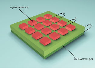
Figure 1: Schematic view of the 2D JJA in dissipative environment.

II.2 Method

To study the JJA model we can use a description in terms of an effective Ginzburg-Landau functional derived from the microscopic model Eq. (2). Several studies of JJA have followed this way, also known as coarse grained approach first developed by Doniach.doniach Most of existing analytical works on quantum JJA have employed different kinds of mean-field-like approximations which are not reliable for treatment spatial and temporal quantum phase fluctuations which quantum spherical approach captures. Formulation of the problem in terms of the spherical modelberlin ; joyce which was initiated by Kopeć and Josékopec3 leads us to introduce the auxiliary complex field $\psi_{i}$ whose expectation value is proportional to the $\mathbf{S}_{i}\left(\phi\right)$ vector defined by

$$\mathbf{S}_{i}\left(\phi\right)=\left[S_{i}^{x}\left(\phi\right),S_{i}^{y}\left(\phi\right)\right]\equiv\left[\cos\left(\phi_{i}\right),\sin\left(\phi_{i}\right)\right].$$ (7)

Natural consequence definition $\mathbf{S}_{i}\left(\phi\right)$ is the following rigid constraint

$$\left|\mathbf{S}_{i}\left(\phi\right)\right|^{2}=\left[S_{i}^{x}\left(\phi\right)\right]^{2}+\left[S_{i}^{y}\left(\phi\right)\right]^{2}=\cos^{2}\left(\phi_{i}\right)+\sin^{2}\left(\phi_{i}\right)\equiv 1.$$ (8)

The relation in Eq. (8) implies that a weaker condition also applies, namely:

$$\sum_{i}\left|\mathbf{S}_{i}\left(\phi\right)\right|^{2}=N.$$ (9)

Using the Fadeev-Popov method with the Dirac $\delta$ functional we obtain:

$$\mathcal{Z} = \int\left[\prod_{i}\mathcal{D}\psi_{i}\mathcal{D}\psi_{j}^{*}\right]\delta\left(\sum_{i}\left|\psi\left(\tau\right)\right|^{2}-N\right)e^{-\mathcal{S}_{\mathrm{J}}\left[\psi\right]}$$ (10)

$$\times\int\left[\mathcal{D}\phi_{i}\right]e^{-\mathcal{S}_{\mathrm{C}+\mathrm{D}}\left[\phi\right]}\prod_{i}\delta\left[\Re\psi_{i}\left(\tau\right)-S_{i}^{x}\left(\phi\left(\tau\right)\right)\right]$$

$$\times\delta\left[\Im\psi_{i}\left(\tau\right)-S_{i}^{y}\left(\phi\left(\tau\right)\right)\right].$$

It is convenient to employ the functional Fourier representation of the $\delta$ functional to enforce the spherical constraint Eq. (9):

$$\delta\left[x\left(\tau\right)\right]=\int_{-i\infty}^{+i\infty}\left[\frac{\mathcal{D}\lambda}{2\pi i}\right]\exp\left[\int_{0}^{\beta}d\tau\lambda\left(\tau\right)x\left(\tau\right)\right],$$ (11)

which introduces the Lagrange multiplier $\lambda\left(\tau\right)$ thus adding an quadratic term (in $\psi$ field) to the action Eq. (2). To evaluation of the effective action in terms of the $\psi$ to second order in $\psi_{i}\left(\tau\right)$ gives the partition function of the quantum spherical model

$$\mathcal{Z_{\mathrm{QSM}}} = \int\left[\prod_{i}\mathcal{D}\psi_{i}\mathcal{D}\psi_{j}^{*}\right]$$ (12)

$$\times\delta\left(\sum_{i}\left|\psi\left(\tau\right)\right|^{2}-N\right)e^{-\mathcal{S}_{\mathrm{QSA}}\left[\psi\right]}$$

where the action of the effective nonlinear $\sigma$ model reads:

$$\mathcal{S}_{\mathrm{QSA}}\mathrm{\left[\psi,\lambda\right]} = \sum_{\left\langle i,j\right\rangle}\int_{0}^{\beta}d\tau d\tau^{\prime}\left\{\left[J_{ij}\left(\tau\right)\delta\left(\tau-\tau^{\prime}\right)\right.\right.$$ (13)

$$+ \left.\mathcal{W}_{ij}^{-1}\left(\tau,\tau^{\prime}\right)-\lambda\left(\tau\right)\delta_{ij}\delta\left(\tau-\tau^{\prime}\right)\right]\psi_{i}\psi_{j}^{*}$$

$$+ \left.N\lambda\left(\tau\right)\delta\left(\tau-\tau^{\prime}\right)\right\}.$$

Furthermore

$$\mathcal{W}_{ij}\left(\tau,\tau^{\prime}\right) = \frac{\delta_{ij}}{\mathcal{Z}_{0}}\int\left[\prod_{i}\mathcal{D}\phi_{i}\right]e^{i\left[\phi_{i}\left(\tau\right)-\phi_{j}\left(\tau^{\prime}\right)\right]}e^{-\mathcal{S}_{\mathrm{C}+\mathrm{D}}\left[\phi\right]}$$ (14)

$$\equiv \mathcal{W}\left(\tau,\tau^{\prime}\right)\delta_{ij},$$

is the phase-phase correlation function with statistical sum

$$\mathcal{Z}_{0}=\int\left[\prod_{i}\mathcal{D}\phi_{i}\right]e^{-\mathcal{S}_{\mathrm{C}+\mathrm{D}}\left[\phi\right]},$$ (15)

where action $\mathcal{S}_{\mathrm{C}+\mathrm{D}}\left[\phi\right]$ is just a sum electrostatic and dissipative term in Eq. (2). After introducing the Fourier transform of the field

$$\phi_{i}\left(\tau\right)=\frac{1}{N\beta}\sum_{\mathbf{k}}\sum_{n=-\infty}^{+\infty}\phi_{\mathbf{k},n}\exp\left[-\left(i\omega_{n}\tau-\mathbf{k}\mathbf{r}_{i}\right)\right]$$ (16)

with $\omega_{n}=2\pi n/\beta$, $\left(n=0,\pm 1,\pm 2,...\right)$ being the Bose Matsubara frequencies, we can write expression Eq. (14) in form

$$\mathcal{W}\left(\tau,\tau^{\prime}\right) = \frac{1}{\mathcal{Z}_{0}}\int\left[\prod_{\mathbf{k}}\mathcal{D}\phi_{\mathbf{k},n}\phi_{\mathbf{k},n}^{*}\right]\exp\left\{-\frac{1}{4N\beta}\sum_{n=-\infty}^{+\infty}\left[\frac{1}{4E_{C}}\omega_{n}^{2}+\frac{\alpha_{0}}{\pi}\left|\omega_{n}\right|\right]\phi_{\mathbf{k},n}\phi_{\mathbf{k},n}^{*}+\right.$$ (17)

$$\left.+\frac{1}{\beta N}\sum_{n=-\infty}^{+\infty}\left[\phi_{\mathbf{k},n}\left(e^{i\omega_{n}\tau}-e^{-i\omega_{n}\tau^{\prime}}\right)+\phi_{\mathbf{k},n}^{*}\left(e^{-i\omega_{n}\tau}-e^{-i\omega_{n}\tau^{\prime}}\right)\right]\right\}.$$

Using Hubbard-Stratonovich transformation the phase-phase correlation function reads:

$$\mathcal{W}\left(\tau,\tau^{\prime}\right)=\exp\left\{-\frac{1}{\beta}\sum_{n\neq 0}\frac{1-\cos\left[\omega_{n}\left(\tau-\tau^{\prime}\right)\right]}{\frac{1}{8E_{C}}\omega_{n}^{2}+\frac{\alpha_{0}}{2\pi}\left|\omega_{n}\right|}\right\}.$$ (18)

The low temperature properties of the expression $\mathcal{W}^{-1}\left(\omega_{n}\right)$ lead to critical value $\alpha_{0}=2$ [see Appendix A]. Finally, for small frequencies and $\alpha_{0}\leq 2$ inverse of the correlation function Eq. (18) becomes:

$$\mathcal{W}^{-1}\left(\omega_{n}\right)=\frac{1}{8E_{C}}\omega_{n}^{2}+\frac{\alpha_{0}}{2\pi}\left|\omega_{n}\right|$$ (19)

for $\omega_{n}\neq 0$ and $\mathcal{W}^{-1}\left(\omega_{n}\right)=0$ otherwise. In the thermodynamic limit ($N\rightarrow\infty$) the steepest descent methods becomes exact; the condition that the integrand in Eq. (12) has a saddle point $\lambda\left(\tau\right)=\lambda_{0}$, leads to an implicit equation for $\lambda_{0}$:

$$1=\frac{1}{\beta N}\sum_{\mathbf{k}}\sum_{n\neq 0}G\left(\mathbf{k},\omega_{n}\right),$$ (20)

where

$$G^{-1}\left(\mathbf{k},\omega_{n}\right)=\lambda_{0}-J_{\mathbf{k}}+\frac{1}{8E_{C}}\omega_{n}^{2}+\frac{\alpha_{0}}{2\pi}\left|\omega_{n}\right|$$ (21)

with $J_{\mathbf{k}}$ as Fourier transform of the Josephson couplings $J_{ij}$.

III Phase diagrams

A Fourier transform of Eq. (13) in momentum and frequency space enables one to write the spherical constraint Eq. (20) explicitly as

$$1=\frac{1}{\beta}\int_{-\infty}^{+\infty}d\xi\sum_{n\neq 0}\frac{\rho\left(\xi\right)}{\lambda-\xi E_{J}+\frac{1}{8E_{C}}\omega_{n}^{2}+\frac{\alpha_{0}}{2\pi}\left|\omega_{n}\right|}.$$ (22)

As is usual in a spherical model, the critical behavior and the phase transitions boundary crucially depends on the spectrum given by density of states $\rho\left(\xi\right)$ and is determined by the denominator of the summand in the spherical constraint Eq. (22). To proceed, it is desirable to introduce density of states for two dimensional lattice in form

$$\rho\left(\xi\right)=\frac{1}{N}\sum_{\mathbf{k}}\delta\left(\xi-\frac{J_{\mathbf{k}}}{E_{J}}\right).$$ (23)

where $J_{\mathbf{k}}$ is energy dispersion. Problem of computing density of states $\rho_{p/q}^{\square}\left(\xi\right)$ for two-dimensional square lattice with uniform magnetic flux per unit plaquette reduces to the solution of Harper’s equationharper , e.g. relevant for tight-binding electrons on 2D latticehasegawa . Analytical results for density of states for square lattice were presented recentlykopec2 , and based on analytically solving Harper’s equation and receiving dispersion relation $J_{\mathbf{k},p/q}^{\square}$. Influence of the local dissipation effects will be considered on triangular lattice without magnetic field. In that case we can use definition Eq. (23) but the dependence on the wave vector is different and could be described by expression

$$J_{\mathbf{k}}^{\bigtriangleup}=E_{J}\left[\cos\left(k_{x}\right)+2\cos\left(\frac{1}{2}k_{x}\right)\cos\left(\frac{\sqrt{3}}{2}k_{y}\right)\right].$$ (24)

Closed formulas for the density of states are placed in Appendix B. The systems displays a critical point at $\lambda_{0}=G^{-1}\left(\mathbf{k}=0,\omega_{n}=0\right)\equiv\max\left[J\left(\mathbf{k}=0\right)\right]$. This fixes the saddle point value of the Lagrange multiplier, $\lambda$ sticks to that value at criticality ($\lambda=\lambda_{0}$) and stays constant in the whole low temperature phase. By substituting the value of $\lambda_{0}$ to Eq. (22) and after performing the summation over Matsubara frequencies, in $T\rightarrow 0$ limit we obtain the following result:

$$1 = \frac{1}{\pi}\int_{-\infty}^{+\infty}d\xi\frac{\rho\left(\xi\right)}{\sqrt{\left(\frac{\alpha_{0}}{2\pi}\right)^{2}-\frac{J_{0}-\xi E_{J}}{2E_{C}}}}$$ (25)

$$\times\ln\left[\frac{\frac{\alpha_{0}}{2\pi}+\sqrt{\left(\frac{\alpha_{0}}{2\pi}\right)^{2}-\frac{J_{0}-\xi E_{J}}{2E_{C}}}}{\frac{\alpha_{0}}{2\pi}-\sqrt{\left(\frac{\alpha_{0}}{2\pi}\right)^{2}-\frac{J_{0}-\xi E_{J}}{2E_{C}}}}\right].$$

It is easy to see that by specifying density of states $\rho\left(\xi\right)$ Eq. (23) with the Coulomb energy $E_{C}$ Eq. (3) for given superconducting network without and in presence of the external magnetic field, we are able to study the zero temperature JJA phase diagram. The solutions and boundary cases above equation we will examine in the next subsections.

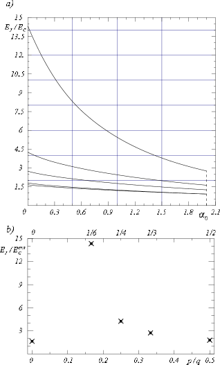
Figure 2: a) Zero temperature phase diagram for the total charging energy $E_{J}/E_{C}$ vs parameter of dissipation $\alpha_{0}$ for square lattice. Insulating state is below the curve. From the top we have $p/q=\frac{1}{6},\frac{1}{4},\frac{1}{3},\frac{1}{2}$ and $0$ b) Nonmonotonical dependence the critical value of the inverse Coulomb energy $E_{J}/E_{C}^{crit}$ for several ratio of the magnetic fluxes $p/q=0,\frac{1}{2},\frac{1}{3},\frac{1}{4}$ and $\frac{1}{6}$.

III.1 Small $\alpha_{0}$ limit

In the limit $\alpha_{0}\rightarrow 0$ expression (25) reduces to zero-temperature critical line in absence dissipation effects:

$$1=\int_{-\infty}^{+\infty}d\xi\rho\left(\xi\right)\sqrt{\frac{2E_{C}}{J_{0}-\xi E_{J}}},$$ (26)

which is according with previous calculationskopec1 . When $\alpha_{0}$ is nonzero, but still small, the situation changes due to a dissipation is a factor which produces additional quantum fluctuations. In consequence for small $\alpha_{0}$ the critical value $E_{J}/E_{C}$ decreases as:

$$E_{J}/E_{C} = A_{0}^{2}-\left(\frac{2}{\pi^{2}}\frac{A_{1}}{A_{0}}\right)^{2}\alpha^{2}+\frac{2}{A_{0}}\left(\frac{2}{\pi^{2}}\frac{A_{1}}{A_{0}}\right)^{3}\alpha^{3}+$$ (27)

$$-\frac{5}{A_{0}^{2}}\left(\frac{2}{\pi^{2}}\frac{A_{1}}{A_{0}}\right)^{4}\alpha^{4}+\mathcal{O}\left(\alpha^{5}\right),$$

where corresponding coefficients reads:

$$A_{0} = \sqrt{2}\int_{-\infty}^{+\infty}d\xi\frac{\rho\left(\xi\right)}{\sqrt{J_{0}/E_{J}-\xi}},$$ (28)

$$A_{1} = \int_{-\infty}^{+\infty}d\xi\frac{\rho\left(\xi\right)}{J_{0}/E_{J}-\xi}.$$ (29)

DOS	$\rho^{\vartriangle}$	$\rho_{0}^{\square}$	$\rho_{1/2}^{\square}$	$\rho_{1/3}^{\square}$	$\rho_{1/4}^{\square}$	$\rho_{1/6}^{\square}$
$A_{0}$	$1.01087$	$1.28576$	$1.34085$	$1.65397$	$2.06193$	$3.78672$
$A_{1}$	$1.92619$	$5.82281$	$4.83852$	$11.8065$	$19.1268$	$175.717$

Table 2: Factors of the expansion critical values $E_{J}/E_{C}$ for small dissipation parameter $\alpha_{0}$ (Eq. 28, 29).

The numerical values of the factors $A_{0}$ and $A_{1}$ are classified in the Table (1). For small ratio $E_{J}/E_{C}$ there is no chance to mobility both Cooper’s pairs and single electrons. If we increase the Josephson energy (or decrease Coulomb energy) we induce phase transitions between insulating and superconducting phase. We have global coherence state but in which there is no single electrons dynamics. The critical values of the inverse Coulomb energy $E_{J}/E_{C}^{crit}$ for $\alpha_{0}=0$ are depicted in Fig.2b) for several values of the magnetic field and are simply equal the first coefficient of the expansion Eq. (27): $\left.E_{J}/E_{C}^{crit}\right|_{\alpha_{0}=0}=A_{0}^{2}$. We note the non-monotonic dependence of the Coulomb energy on the magnetic flux ratio $p/q$.

III.2 Critical value $\alpha_{0}$

At zero temperature dissipation suppresses quantum fluctuations entirely and drives system to a global coherent state. Due to the fact, that correlation function Eq. (18) for low temperatures: $\mathcal{W}^{-1}\left(\omega_{n}\right)\sim\left|\omega_{n}\right|^{\frac{2}{\alpha_{0}}-1}$ becomes divergent for $\alpha_{0}\geq 2$ [see Appendix A], the critical lines are cut at this point what is depicted on phase diagrams in Fig.2a and Fig.3. This boundary value $\alpha_{0}$ does not depend on magnetic field and on the geometry of the network. It seems to be universal for different types of lattices without and in presence of the external magnetic field. The system behaves as if it were classical because of the big contribution to the action Eq. (2) which is generated by large values of the dissipation parameter $\alpha_{0}$. Dissipation can correlate the phase on a single island in different time and this correlation has the biggest impact on global coherent state when $\alpha_{0}$ is greater then critical value. Similar behaviour of the phase diagrams with critical value of the dissipation parameter was predicted by several authors.chakravaraty ; fisher1 ; wagenblast Theory developed by Chakravaraty et al.chakravaraty reveals, that phase transition takes place at point $\alpha_{\mathrm{crit}}=1/d$ where $d$ is the dimension of the system. The insulating phase disappears for $\alpha_{0}>2$ in model considered by Wagenblast et al.wagenblast , the authors claim that dissipative processes completely suppress the phase fluctuations. Kampf and Schönkampf1 using variational procedure showed that different mechanisms: Ohmic and quasi-particle damping lead to different critical values of $\alpha_{0}$. In magnetic field the dependence of critical temperature on several ratio of the magnetic fluxes is periodic with period $1$ and symmetric around $p/q=1/2$.kampf Note that phase diagrams for different lattice geometry and in presence of a magnetic field with effects of the local dissipation has not been presented.

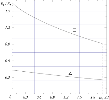
Figure 3: Zero temperature phase diagram for the normalized Josephson energy $E_{J}/E_{C}$ vs parameter of dissipation $\alpha_{0}$ for square and triangular lattice. Insulating state is below the curves.

IV Summary

We have studied the ground phase diagram two-dimensional Josephson junction arrays in quantum regime by analytical methods using the quantum-spherical approach with exactly evaluated density of states for square and triangular lattice. For square lattice we could take into consideration perpendicular magnetic field which was described by rational magnetic flux $f=p/q$ for a number of values $1/q$. Zero temperatures phase diagram indicates that for small values $\alpha_{0}$ quantum fluctuations destroy the long-range phase coherence. The arrays can be in two phases: Mott-insulator phase and global coherent state. We can travel between phases vary Coulomb energy or dissipation parameter. When $\alpha_{0}$ is greater than critical value, the dissipation suppresses quantum fluctuations and the array orders even for small ratio $E_{J}/E_{C}$. Why dissipation can restore global coherent state? If we imagine that we allow electrons tunnel between superconducting arrays and metallic substrate, remaining Cooper’s pairs will become more mobile too. Therefore we will not be equal to set a number pair on the island. Because superconducting phase $\phi$ and the number of Cooper’s pair $\hat{n}$ follow uncertainty relation $\left[\phi,\hat{n}\right]=2i$ then if we cannot say anything about quantity of Cooper’s pair on the island the phase is determined and in consequence we obtain global coherent state. In case when system is in presence of the magnetic field damping is stronger than in the absence. If we vary flux parameter $f=p/q$ we could drive array into insulating state. Magnetic field could affect the dissipation because it influences the resistance of at least the coherent parts and thus changes the effective shunting. For small values dissipation parameter $\alpha_{0}$ Josephson energy in triangular lattice is damped less then for square lattice even in presence magnetic field. We can notice that if the quantum fluctuations of the phase superconducting order parameter are important, the dissipation plays decisive role in constitute the onset of global superconductivity.

Appendix A Low Temperature Properties of the corellator

We write correlation function Eq. (18) in form:

$$\mathcal{W}\left(\tau\right)=\exp\left\{-\frac{1}{\beta}\sum_{n\neq 0}\frac{1-\cos\left(\omega_{n}\tau\right)}{\frac{1}{8E_{C}}\omega_{n}^{2}+\frac{\alpha_{0}}{2\pi}\left|\omega_{n}\right|}\right\}$$ (30)

and observe that the sum over $\omega_{n}$ is symmetric when we change $\omega_{n}\rightarrow-\omega_{n}$. In that case (getting rid of abs) we can write

$$\mathcal{W}\left(\tau\right)=\exp\left\{-\frac{2}{\beta}\sum_{n\geq 1}\frac{1-\cos\left(\omega_{n}\tau\right)}{\frac{1}{8E_{C}}\omega_{n}^{2}+\frac{\alpha_{0}}{2\pi}\omega_{n}}\right\}$$ (31)

noticing then sums over $n\geq 1$ and $n\leq 1$ are the same. Now we are splitting above expression for two parts and neglecting the $\omega_{n}^{2}$ in second contribution (in low temperatures more important is part which contains $\omega_{n}$) we get:

$$\mathcal{W}\left(\tau\right)=\exp\left[-\frac{2}{\beta}\sum_{n\geq 1}\frac{1}{\frac{1}{8E_{C}}\omega_{n}^{2}+\frac{\alpha_{0}}{2\pi}\omega_{n}}\right]\exp\left[\frac{2}{\beta}\sum_{n\geq 1}\frac{\cos\left(\omega_{n}\tau\right)}{\frac{\alpha_{0}}{2\pi}\omega_{n}}\right].$$ (32)

Evaluating the sums we can write:

$$\mathcal{W}\left(\tau\right)=\exp\left[-\frac{1}{\alpha_{0}}\mathbf{H}\left(\frac{8\beta E_{C}}{\alpha_{0}}\right)\right]\exp\left\{\frac{2}{\alpha_{0}}\log\left[2\sin\left(\frac{\pi}{\beta}\left|\tau\right|\right)\right]\right\},$$ (33)

and using asymptotic relation (valid for $\beta\rightarrow\infty$) of the harmonic number function $\mathbf{H}\left(n\right)=\sum_{i=1}^{n}i^{-1}$:

$$\mathbf{H}\left(a\beta\right)=\ln a\beta+\gamma+\frac{1}{2}a\beta-\frac{1}{12}\left(\frac{1}{a\beta}\right)^{2}+\frac{1}{120}\left(\frac{1}{a\beta}\right)^{4}+...\mathcal{O}\left(\frac{1}{\beta^{6}}\right),$$ (34)

where $\gamma$ is Euler’s constant, finally we have found

$$\mathcal{W}^{-1}\left(\tau\right)=\exp\left(\frac{\gamma}{\alpha_{0}}\right)\left(2\frac{\pi}{\beta}\left|\tau\right|\right)^{-\frac{2}{\alpha_{0}}}.$$ (35)

After Fourier transform correlator becomes:

$$\mathcal{W}^{-1}\left(\omega_{n}\right)=\exp\left(\frac{\gamma}{\alpha_{0}}\right)\Gamma\left(1-\frac{2}{\alpha_{0}}\right)\sin\left(\frac{\pi}{\alpha_{0}}\right)\left|\omega_{n}\right|^{\frac{2}{\alpha_{0}}-1},$$ (36)

besides the Euler gamma function $\Gamma\left(z\right)$ is defined by the integral:abramovitz

$$\Gamma\left(z\right)=\int_{0}^{\infty}t^{z-1}e^{-t}dt \Re z>0.$$ for (37)

and can be viewed as a generalization of the factorial function, valid for complex arguments. Finally we can see that correlator

$$\mathcal{W}^{-1}\left(\omega_{n}\right)\sim\left|\omega_{n}\right|^{\frac{2}{\alpha_{0}}-1}$$ (38)

at zero temperature diverges for $\alpha_{0}\geq 2$.

Appendix B Density of States

In the case of zero magnetic field the density of states for the square two-dimensional lattice reads simply

$$\rho_{0}^{\square}\left(\xi\right)=\frac{1}{\pi^{2}}\mathbf{K}\left(\sqrt{1-\left(\frac{\xi}{2}\right)^{2}}\right)\Theta\left(1-\left|\frac{\xi}{2}\right|\right),$$ (39)

where

$$\mathbf{K}\left(x\right)=\int_{0}^{\pi/2}\frac{d\phi}{\sqrt{1-x^{2}\sin^{2}\phi}},$$ (40)

is the elliptic integral of the first kindabramovitz and the unit step function is defined by:

$$\Theta\left(x\right)=\left\{\begin{array}[]{ccc}1&\textrm{for}&x>0\\ 0&\textrm{for}&x\leq 0\end{array}\right..$$ (41)

The procedure obtaining closed formulas for density of states in presence of the magnetic field based on analytically solving Harper’s equation. The Harper’s equation was studied intensivelyhasegawa1 ; gumbs ; hong but only on numerical way and was missed analytic closed formulas for density of states in presence of the magnetic field. Only expression for case $p/q=1/2$ was received by Tan and Thouless and also was formulated in terms of the elliptic integrals.tan Therefore the density of states for square lattice with the magnetic quantum flux per plaquette for value $p/q=\frac{1}{2}$ reads:kopec2

$$\rho_{1/2}^{\square}\left(\xi\right)=\frac{\left|\xi\right|}{2}\rho_{0}^{\square}\left(\frac{\xi^{2}-4}{2}\right).$$ (42)

It is only one gap-less case instead of $p/q=0$.

Obtaining closed formulas for the next case $p/q=1/3$ was more difficult, and we have got following expression

$$\rho_{1/3}^{\square}\left(\xi\right) = \frac{1}{4\sqrt{2}}\left|\xi^{2}-2\right|\sqrt{\xi^{2}-8}\rho_{0}^{\square}\left[\frac{1}{2}\xi\left(\xi^{2}-6\right)\right]$$ (43)

$$\times\left\{\left|\sec\left(\alpha+\frac{\pi}{2}\right)\right|\left[\Theta\left(\xi+1+\sqrt{3}\right)-\Theta\left(6-\xi^{2}\right)-\Theta\left(\xi-1-\sqrt{3}\right)\right]\right.$$

$$+\sec\left(\alpha+\frac{\pi}{6}\right)\left[\Theta\left(\xi+\sqrt{6}\right)-\Theta\left(\xi+2\right)+\Theta\left(\xi\right)-\Theta\left(\xi+1-\sqrt{3}\right)\right]$$

$$\left.+\sec\left(\alpha+-\frac{\pi}{6}\right)\left[\Theta\left(\xi-1+\sqrt{3}\right)-\Theta\left(\xi\right)+\Theta\left(\xi-2\right)\Theta\left(\xi-\sqrt{6}\right)\right]\right\},$$

where

$$\alpha=\frac{1}{3}\arctan\left(\frac{\sqrt{32-\xi^{2}\left(\xi^{2}-6\right)^{2}}}{\xi\left(\xi^{2}-6\right)}\right).$$ (44)

For $p/q=1/4$ the expression for density of states is straightly given by:

$$\rho_{1/4}^{\square}\left(\xi\right) = \frac{1}{2}\left|\xi^{2}-4\right|\rho_{0}^{\square}\left[\frac{1}{2}\left(\xi^{4}-8\xi^{2}+4\right)\right]\left\{\sqrt{4+\left|\xi^{2}-4\right|}\left[\Theta\left(8-\xi^{2}\right)-\Theta\left(4+2\sqrt{2}-\xi^{2}\right)\right]\right.$$ (45)

$$\left.+\sqrt{4-\left|\xi^{2}-4\right|}\Theta\left(4-2\sqrt{2}-\xi^{2}\right)\right\}.$$

Finally the most complicated case $p/q=1/6$ with six symmetric singularities divide symmetrically on the positive and negative part of the axis $\xi$:

$$\rho_{1/6}^{\square}\left(\xi\right) = \frac{1}{4\sqrt[4]{2}}\left|\xi^{4}-8\xi^{2}+8\right|\sqrt{\xi^{4}-8\xi^{2}-16}\rho_{0}^{\square}\left[\frac{1}{2}\left(\xi^{2}-6\right)\right]$$ (46)

$$\times\left\{\left|\sec\left(\alpha+\frac{\pi}{2}\right)\right|\left[\Theta\left(\xi+1+\sqrt{3}\right)-\Theta\left(6-\xi^{2}\right)-\Theta\left(\xi-1-\sqrt{3}\right)\right]\right.$$

$$+\sec\left(\alpha+\frac{\pi}{6}\right)\left[\Theta\left(\xi+\sqrt{6}\right)-\Theta\left(\xi+2\right)+\Theta\left(\xi\right)-\Theta\left(\xi+1-\sqrt{3}\right)\right]$$

$$\left.+\sec\left(\alpha+-\frac{\pi}{6}\right)\left[\Theta\left(\xi-1+\sqrt{3}\right)-\Theta\left(\xi\right)+\Theta\left(\xi-2\right)\Theta\left(\xi-\sqrt{6}\right)\right]\right\},$$

where

$$\alpha=\frac{1}{3}\arctan\left(\frac{\left|\left(\xi^{4}-8\xi^{2}+8\right)\sqrt{16+8\xi^{2}-\xi^{4}}\right|}{\xi^{6}-12\xi^{4}+24\xi^{2}+32}\right).$$ (47)

The density of states for triangular lattice with six nearest neighbors we can write in form:

$$\rho^{\bigtriangleup}\left(\xi\right)=\frac{2}{\pi^{2}\sqrt{\kappa_{0}}}\mathbf{K}\left(\sqrt{\frac{\kappa_{1}}{\kappa_{0}}}\right)\left[\Theta\left(\xi+\frac{3}{2}\right)-\Theta\left(\xi-3\right)\right],$$ (48)

where

$$\kappa_{0}=\left(3+2\sqrt{3+2\xi}-\xi^{2}\right)\left[\Theta\left(\xi+\frac{3}{2}\right)-\Theta\left(\xi+1\right)\right]+4\sqrt{3+2\xi}\left[\Theta\left(\xi+1\right)-\Theta\left(\xi-3\right)\right],$$ (49)

$$\kappa_{1}=4\sqrt{3+2\xi}\left[\Theta\left(\xi+\frac{3}{2}\right)-\Theta\left(\xi+1\right)\right]+\left(3+2\sqrt{3+2\xi}-\xi^{2}\right)\left[\Theta\left(\xi+1\right)-\Theta\left(\xi-3\right)\right].$$ (50)

References

- (1) B. Abeles, Phys. Rev. B 15, 2828 (1977).
- (2) E. S̆imánek, Solid State Commun. 31, 419 (1979).
- (3) E. S̆imánek, Phys. Rev. B 22, 459 (1980); 23, 5762 (1982); 32, R500 (1985).
- (4) S. Doniach, Phys. Rev. B 24, 5063 (1981).
- (5) R. M. Bradley and S. Doniach, Phys. Rev. B 30, 1138 (1984).
- (6) D. M. Wood and D. Stroud, Phys. Rev. B 25, 1600 (1982).
- (7) T. K. Kopeć and J. V. José, Phys. Rev. B 63, 064504 (2001).
- (8) J. V. José, Phys. Rev. B 29, R2836 (1984); L. Jacobs, J. V. José and M. A. Novotny, Phys. Rev. Lett. 53, 2177 (1984).
- (9) T. K. Kopeć and T. P. Polak, Phys. Rev. B 66, 094517 (2002).
- (10) R. F. Voss and R. A. Webb, Phys. Rev B 25, R3446 (1982).
- (11) B. J. van Wees, H. S. J. van der Zant, and J. E. Mooij, Phys. Rev. B 35, R7291 (1987).
- (12) H. S. J. van der Zant, W. J. Elion, L. J. Geerligs, and J. E. Mooij, Phys. Rev. B 54, 10081 (1996).
- (13) P. Caputo, M. V. Fistul, and A. V. Ustinov, Phys. Rev. B 63, 214510 (2001).
- (14) C. Bruder, R. Fazio, and G. Schön, Phys. Rev. B 47, 342 (1993); T. K. Kopeć and J. V. José, Phys. Rev. B 60, 7473 (1999), G. Grignani, A. Mattoni, P. Sodano, A. Trombettoni, Phys. Rev. B 61, 11676 (2000); W. A. Al-Saidi and D. Stroud, Phys. Rev. B 67, 024511 (2003); W. A. Al-Saidi and D. Stroud, Physica C 402, 216, (2004).
- (15) A. O. Caldeira and A. J. Leggett, Phys. Rev. Lett. 46, 211 (1981); Ann. Phys. 149, 374 (1983).
- (16) G. Schön, A. D. Zaikin, Phys. Rep. 198, 237 (1990).
- (17) V. Ambegaokar, U. Eckern and G. Schön, Phys. Rev. Lett. 48, 1745 (1982).
- (18) S. Chakravarty, G. L. Ingold, S. Kivelson, and A. Luther, Phys. Rev. Lett. 56, 2303 (1986); S. Chakravarty, G. L. Ingold, S. Kivelson, and G. Zimányi, Phys. Rev. B 37, 3283 (1988).
- (19) M. P. A. Fisher, Phys. Rev. Lett. 57, 885 (1986); S. Chakravarty, S. Kivelson, G. T. Zimányi, and B. I. Halperin, Phys. Rev. B 35, R7256 (1987).
- (20) E. S̆imánek and R. Brown, Phys. Rev. B 34, R3495 (1986).
- (21) M. P. A. Fisher, Phys. Rev. B 36, 1917 (1987).
- (22) W. Zwerger, J. Low Temp. Phys. 72, 291 (1988).
- (23) S. V. Panyukov, A. D. Zaikin, J. Low Temp. Phys. 75, 365 (1989); 75, 389 (1989).
- (24) S. Chakravarty, G. L. Ingold, S. Kivelson, A. Luther, Phys. Rev. Lett. 56, 2303 (1986).
- (25) S. Chakravarty, G. L. Ingold, S. Kivelson, G. Zimányi, Phys. Rev. B 37, 3283 (1988).
- (26) G. Falci, R. Fazio, G. Giaquinta, Europhys. Lett. 14, 145 (1991).
- (27) A. Cuccoli, A. Fubini, V. Tognetti, R. Vaia, cond-mat=0002072.
- (28) U. Eckern, G. Schön and V. Ambegaokar, Phys. Rev. B 30, 6419 (1984).
- (29) A. Kampf, G. Schön, Physica 152, 239 (1988); A. Kampf, G. Schön, Phys. Rev. B 36, 3651 (1987); E. S̆imánek and R. Brown, Phys. Rev. B 34, R3495 (1986).
- (30) J. Choi and J. V. José, Phys. Rev. Lett. 62, 1904 (1989).
- (31) A. Kampf and G. Schön, Phys. Rev. B 37, R5954 (1988).
- (32) S. Kim and M. Y. Choi, Phys. Rev. B 42, 80 (1990).
- (33) H. Beck, Phys. Rev. B 49, 6153 (1994); S. E. Korshunov, Phys. Rev. B 50, 13616 (1994); K. H. Wagenblast, A. van Otterlo, G. Schön, G. T. Zimányi, Phys. Rev. Lett. 79, 2730 (1997).
- (34) L. J. Geerligs, M. Peters, L. E. M. de Groot, A. Verbruggen, and J. E. Mooij, Phys. Rev. Lett. 63, 326 (1989); A. F. Hebard and M. A. Paalanen, Phys. Rev. Lett. 65, 927 (1990); A. J. Rimberg, T. R. Ho, Ç. Kurdak, J. Clarke, K. L. Campman, A. C. Gossard, Phys. Rev. Lett. 78, 2632 (1997).
- (35) J. M. Valles, Jr. R. C. Dynes, and J. P. Garno, Phys. Rev. Lett. 69, 3567 (1992);
- (36) A. Yazdani and A. Kapitulnik, Phys. Rev. Lett. 74, 3037 (1995).
- (37) R. Fazio and G. Schön, Phys. Rev. B 43, 5307 (1991).
- (38) C. C. Homes, S. V. Dordevic, M. Strongin, D. A. Bonn, Ruixing Liang, W. N. Hardy, Seiki Komiya, Yoichi Ando, G. Yu, N. Kaneko, X. Zhao, M. Greven, D. N. Basov, T. Timusk, Nature, 430, 539 - 541 (2004).
- (39) W. H. Zurek, Phys. Today, 44, 36 (1991); D. Braun, F. Haake, W. T. Strunz, Phys. Rev. Lett. 86, 2913 (2001).
- (40) S. Han, Y. Yu, X. Chu, S. Chu, Z. Wang, Science, 293, 1457 (2001).
- (41) W. Y. Shih and D. Stroud, Phys. Rev. B 30, R6774 (1984).
- (42) E. Granato and J. M. Kosterlitz, Phys. Rev. Lett. 65, 1267 (1990).
- (43) S. P. Benz, M. S. Rzchowski, M. Tinkham and C. J. Lobb, Phys. Rev. Lett. 64, 693 (1990).
- (44) M. Abramovitz and I. Stegun, Handbook of Mathematical Functions (Dover, New York, 1970).
- (45) T. H. Berlin and M. Kac, Phys. Rev. B 86, 821 (1952); H. E. Stanley, Phys. Rev. B 176, 718 (1968).
- (46) G. S. Joyce Phys. Rev. B 146, 349 (1966).
- (47) The spherical model in general reveals, in a simplified way, the failure of mean field theory below the upper critical dimension. For example, in the classical spherical model, the critical exponent of the correlation length is which differs from the mean field value , which is dimensionality independent. Spherical model also predicts that critical temperature is vanishing to zero if dimensionality of the system is less then two, which is not suprising according to Mermin-Wagner theorem.
- (48) K. H. Wagenblast, A. van Otterlo, G. Schön and G. T. Zimányi, Phys. Rev. Lett. 78, 1779 (1997).
- (49) T. K. Kopeć, J. V. José, Phys. Rev. B 60, 7473 (1999).
- (50) P. G. Harper, Proc. Phys. Soc. London Sect. A 68, 674 (1955).
- (51) Y. Hasegawa, P. Lederer, T. M. Rice, P. B. Wiegmann, Phys. Rev. Lett. 63, 907 (1984).
- (52) Y. Hasegawa, Y. Hatsugai, M. Kohmoto and G. Montambaux, Phys. Rev. B 41, 9174 (1990).
- (53) G. Gumbs and P. Fekete, Phys. Rev. B 56, 3787 (1997).
- (54) S. P. Hong and S.-H. S. Salk, Phys. Rev. B 60, 9550 (1999).
- (55) Y. Tan and D. J. Thouless, Phys. Rev. B 46, 2985 (1992).