Ultra-cold fermions in optical lattices

Abstract

We summarize recent theoretical results for the signatures of strongly correlated ultra-cold fermions in optical lattices. In particular, we focus on: collective mode calculations, where a sharp decrease in collective mode frequency is predicted at the onset of the Mott metal-insulator transition; and correlation functions at finite temperature, where we employ a new exact technique that applies the stochastic gauge technique with a Gaussian operator basis.

1 Introduction

Recent progress in obtaining bosonic and fermionic quantum gases has ushered in a new experimental paradigm in physics. An essential feature in these developments is that, although technically challenging, ultra-cold atom experiments have remarkably simple physical conditions. The significant issues are that:

• the underlying interactions are well understood,

• there are few parameters needed

• interactions can be tuned in many cases

This will greatly help our understanding of many-body physics, since precise theoretical models can be readily obtained at low density, without the complications of a crystal lattice and reservoirs – as is so often the case at present.

Thus, one can apply simple theoretical models with high accuracy, allowing innovative experimental tests of methods in quantum field theory (QFT). This could lead to novel fundamental experiments in physics, such as tests of massive particle quantum entanglement, as well as applications to metrology.

An important element in recent investigations is the technique of coherent transformation of cold atoms to molecules, either using photo-association[1] or Feshbach[2] resonance methods. This allows a strong, tunable interaction between the atoms. Experiments have confirmed coherently coupled atom-molecular models[3], with renormalization[4].

Bosonic molecular experiments include ¹³³Cs, ⁸⁷Rb, and ²³Na [5]. Fermi gases of ⁴⁰K and ⁶Li atoms have proved to be ideal experimental systems owing to their long molecular lifetimes[6]. These have resulted in cold molecule production[7], molecular Bose-Einstein condensation[8], and preliminary indications of fermion superfluid behaviour [9, 10].

The properties of ultracold Bose gases in optical lattices[11] are another ‘hot’ topic, as a starting point for the exploration of strongly correlated many-body systems[12, 13]. Fermionic experiments in optical lattices are already underway[14], thus allowing the direct realization of the strongly coupled lattice of fermions known as the Hubbard model. In this paper we review some recently obtained results for the Hubbard model, in particular:

• the use of collective modes as signatures for the metal-insulator phase-transition

• a new exact Gaussian technique for calculating finite temperature correlation functions, without the Fermi sign problem of traditional Monte-Carlo methods.

2 Hubbard model

A one-dimensional, sinusoidal optical potential is easily created for trapped atoms. The results are different for fermions and for bosons, since because of the Pauli exclusion principle, at least two distinct spin eigenstates are needed to have on-site interactions with fermions.

This leads to the (fermionic) Hubbard model,

$$\mathcal{H}=-\sum\limits_{j,\sigma=\pm 1}t_{ij}\left(\widehat{a}_{i,\sigma}^{\dagger}\widehat{a}_{j,\sigma}+h.c.\right)+U\sum_{j}\widehat{n}_{j,+}\widehat{n}_{j,-}+\sum_{j,\sigma=\pm 1}V_{j}\widehat{n}_{j,\sigma}\,\,,$$ (1)

where $V_{j}$ includes the external trap potential which we assume is harmonic, $U$ gives rise to on-site interactions, and $t_{ij}$ describes tunneling between the sites. This model of interacting fermions is also used in high-$T_{c}$ superconductivity, where it is more qualitative than quantitative in its applicability. The dimensionality and lattice structure of the model determine the tunneling matrix $t_{ij}$. In most of the paper, we will assume this is a one-dimensional lattice with $t_{ij}=t\delta_{i+1,j}$, and $V_{j}=m\omega_{0}^{2}d^{2}j^{2}/2$, where $m$ is the fermion mass, $\omega_{0}$ the trap frequency, and $d$ the well-separation. We also give correlation results for two-dimensional lattices in the last section.

2.1 Band structure

In a single-band model as given above, one can expect a band insulator to form in the non-interacting limit, when all available sites have been occupied (i.e., two particles per site). However, this is complicated by the existence of the external potential. For a large, deep trap, the density increases towards the centre, so that the insulating region becomes localised, coexisting with a conducting region in the wings.

When there are strong repulsive on-site interactions, the system develops a new band structure in which an insulating region forms at half-filling, i.e., with only one particle per site. This is shown in Figure (1).

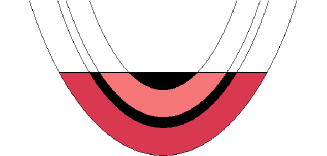
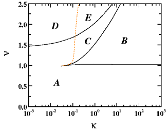
Figure 1: Left graph: schematic illustration of effective single-particle band structure in a harmonically trapped fermionic Hubbard model. Right graph: phase-diagram vs the coupling ($\kappa$ ) and filling ($\nu$ ). For details see Section (2.2).

2.2 Local Density Approximation

In the local density approximation (LDA), we assume that the trap is slowly varying compared to all correlation length scales. This allows us to use the piecewise exact solution for the uniform 1D Hubbard model[15] to describe the strongly-correlated interacting ground state.

It most useful to introduce an effective mass and frequency, corrected for the band-dispersion, as well as a dimensionless coupling constant and filling factor, where:

• Effective mass, frequency: $\,m^{*}=\hbar^{2}/\left(2td^{2}\right)$, $\,\omega=\hbar\omega_{0}\left(m/m^{*}\right)^{1/2}/t$

• Coupling constant $\,\kappa=U^{2}/\left(8t^{2}N\omega\right)$

• Effective filling factor $\,\nu=\sqrt{2N\omega}/\pi$

The effective filling factor can be understood as corresponding to a single particle per site ($n=1$) at the trap centre for $\nu=1$, although the interpretation is more complex in general, due to the effects of the trap potential. Note that $\nu$ is defined as a global parameter for the entire trap, while the occupation per site ($n$) varies with radius.

With these parameters, and using the LDA, with a fixed global chemical potential and harmonic trap potential, one obtains a phase-diagram[16, 17] as shown in the right-hand diagram in Fig (1). The labelled regions are as follows:

$A$: a pure metallic phase. In this case there are no filled bands, and the quantum gas behaves analogously to a metallic conductor, with $n<2$ everywhere.

$B$: a single Mott insulator domain at the center, accompanied by two metallic wings. Here the strong particle-particle interactions prevent occupation numbers larger than one, even though these are allowed by the Pauli principle.

$C$: a metallic phase at the center surrounded with Mott insulator plateaus. In this case, a larger particle number opens up a second band in the trap center, in which higher occupations with $n>1$ are possible.

$D$: a band insulator at the center with metallic wings outside. This is similar to phase B. Here, however, due to weaker inter-particle interactions there is no Mott phase, and the central band insulator with $n=2$ is caused purely by the Pauli exclusion principle.

$E$: a band insulator at the trap center surrounded by metallic regions, in turn surrounded by Mott insulators. In this case there is a large particle number and strong interactions, so both Mott insulator and band insulator regions can occur at different radii from the centre.

3 Collective mode frequencies

3.1 Luttinger approximation

In order to describe the collective modes, we can make use of the Luttinger long-wavelength Hamiltonian[13], valid for small displacements. Because of the spin-density separation in the Hamiltonian, there are two types of waves present, described by the indices $\nu=\rho,\sigma$. We assume here that the external potential only depends on the density, and does not transform one type of wave into the other, so that the inhomogeneous Hamiltonian is:

$${\mathcal{H}}_{\textrm{LL}}=\sum_{\nu=\rho,\sigma}\int dx\frac{u_{\nu}(x)}{2}\left[K_{\nu}(x)\Pi_{\nu}^{2}+\frac{1}{K_{\nu}(x)}\left(\frac{\partial\phi_{\nu}}{\partial x}\right)^{2}\right]\,\,.$$ (2)

Here the density and spin-wave velocities are $u_{\rho}$, $u_{\sigma}$respectively, and these have Luttinger exponents $K_{\rho}$, $K_{\sigma}$. Using the LDA, we can therefore solve the resulting wave-equations for the collective mode frequency, with zero-current boundary conditions at the boundaries where the density vanishes[18].

The results are shown in Fig (2), in which we have solved for the collective fermionic modes in a trapped one-dimensional two-component Fermi gas, together with an optical lattice[17]. These graphs show a sharp frequency dip as an unmistakable signature of Mott metal-insulator transition (MMIT) physics. This occurs just at the filling factor where the insulating region starts to form at the trap centre.

The reason for this is simple to understand. Collective modes involve large density currents, which propagate through the lattice with a characteristic velocity $u_{\rho}$. However, these velocities tend to zero in the neighborhood of an insulating region, and must be exactly zero inside the insulator. This effect slows down transport processes and therefore reduces all collective mode frequencies, which scale as $velocity/length$. The effect is strongest just when the insulating region starts to form, leading to a large fraction of the conducting region having a low average velocity. As the insulating region grows, the part of the trap that is conducting is localized to the wings, so the frequency increases again due to the smaller characteristic lengths involved.

However, there are some limitations to these methods. In particular, this is a linearized method, and hence is only valid for small displacements; it also only applies to zero temperature.

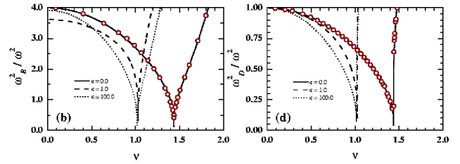
Figure 2: Breathing ($\omega_{B}$) and dipole ($\omega_{D}$) mode frequency vs filling factor $\nu$ for zero, intermediate and strong couplings.

Preliminary results in the non-interacting case using the Boltzmann equations (circles in Fig (2)) show that there are additional damping effects that are proportional to displacement. This leaves an unsolved problem, of how to deal with finite temperatures and large displacements in the interacting case.

4 Quantum simulation with Gaussian operators

We now turn to the question of how to carry out many-body quantum field theory calculations without approximations. Quantum Monte-Carlo (QMC) techniques for fermionic problems are strongly limited by the Fermi sign problem, which causes large sampling errors[19].

Here we give some results using a novel method constructed from a basis of Gaussian operators, which treats covariances (Green’s functions) as phase-space variables. In principle, this method can simulate both fermions and bosons[20], including either thermal ensembles and dynamics. We will treat the case of finite-temperature fermionic ensembles for definiteness.

4.1 Gaussian expansion

Our approach is different from traditional QMC methods. We expand the state density operator $\,\widehat{\rho}$ in an operator basis $\,\widehat{\Lambda}$:

$$\,\widehat{\rho}=\int P(\overrightarrow{\lambda})\widehat{\Lambda}(\overrightarrow{\lambda})d\overrightarrow{\lambda}\,\,,$$ (3)

where $P(\overrightarrow{\lambda})$ is a probability distribution, sampled stochastically over the variables$\overrightarrow{\lambda}$ which constitute a phase-space. Time (or inverse temperature) evolution is obtained by a mapping procedure which maps operator equations into stochastic equations:

$$\partial\widehat{\rho}/\partial t=\widehat{L}[\widehat{\rho}] \longrightarrow \partial\overrightarrow{\lambda}/\partial t=\overrightarrow{A}+\mathbf{B}\,\overrightarrow{\zeta}\,\,.$$ (4)

These equations are typically not unique, and have a ‘stochastic gauge’ degree of freedom, which must be chosen to make the distribution compact enough to eliminate boundary terms and minimize sampling errors[21].

4.2 Gaussian operators

The mapping procedure depends on the operator basis chosen, and we shall choose a Gaussian operator basis, defined for both Fermi[22] and Bose[23] cases, as:

$$\,\widehat{\Lambda}_{\pm}(\mathbf{n})=\Omega\left|\mathbf{I}\pm\mathbf{n}\right|^{\mp 1}:\exp\left[\widehat{\mathbf{a}}\left(\mathbf{I}\mp\mathbf{I}-\left[\mathbf{I}\pm\mathbf{n}\right]^{-1}\right)\widehat{\mathbf{a}}^{\dagger}\right]:\,\,.$$ (5)

Here, annihilation and creation operators are included as a vector: $\,\widehat{\mathbf{a}}=\left(\widehat{a}_{1},...,\widehat{a}_{M}\right)^{T}$. The upper signs apply for bosons, the lower signs for fermions.

A typical application of these methods is to calculate thermal equilibrium correlation functions. Since the fermion number is usually unknown, the grand canonical distribution, $\widehat{\rho}=\exp(-(\widehat{H}-\mu\widehat{N})\tau)$, is the most appropriate choice of ensemble. Here, $\widehat{\rho}$ is the unnormalised density operator, $\tau=1/k_{B}T$ is the inverse temperature, and $\mu$ is the chemical potential. The phase-space variable $\mathbf{n}$ is a complex matrix, which is best thought of as a (finite temperature) stochastic Green’s function. Thus, $\left\langle\,\widehat{a}_{i}^{\dagger}\widehat{a}_{j}\right\rangle_{\tau}=\left\langle\Omega n_{ij}\right\rangle_{P(\tau)}$, where $\left\langle.\right\rangle_{P}$ indicates a phase-space average over the distribution $P$.

5 Fermionic correlations

Rewriting the canonical density operator as an equation for inverse temperature evolution, one obtains:

$$\frac{d\widehat{\rho}}{d\tau}=-\frac{1}{2}\left[(\widehat{H}-\mu\widehat{N}),\widehat{\rho}\right]_{+}\,\,.$$ (6)

After applying the appropriate identities, one then obtains the following Stratonovich stochastic gauge equations for the Hubbard model, where $\Omega$ is a weight and $\mathbf{n}_{\sigma}$ is the stochastic Green’s function for spin $\sigma=\pm 1$:

$$\frac{d\Omega}{d\tau} = -\Omega H(\mathbf{n}_{+},\mathbf{n}_{-})$$

$$\frac{d\mathbf{n}_{\sigma}}{d\tau} = \frac{1}{2}\left\{\left(\mathbf{I}-\mathbf{n}_{\sigma}\right)\bm{T}_{\sigma}^{(1)}\!\mathbf{n}_{\sigma}+\mathbf{n}_{\sigma}\bm{T}_{\sigma}^{(2)}\!\left(\mathbf{I}-\mathbf{n}_{\sigma}\right)\right\}\,\,.$$ (7)

Here we have introduced a transition matrix $T_{\sigma}^{(j)}$ and real Gaussian noise terms defined by:

• T-matrix: $\,T_{i,j,\sigma}^{(r)}=t_{ij}-\delta_{i,j}\left\{|U|(sn_{j,j,-\sigma}-n_{j,j,\sigma}+\frac{1}{2})-\mu+\sigma^{(s+1)/2}\xi_{j}^{(r)}\right\},$

• Noises: $\,\left\langle\xi_{j}^{(r)}(\tau)\,\xi_{j^{\prime}}^{(r^{\prime})}(\tau^{\prime})\right\rangle=2|U|\delta(\tau-\tau^{\prime})\delta_{j,j^{\prime}}\delta_{r,r^{\prime}}\,\,$.

5.1 Finite-temperature correlations

The left graph of Fig (3) shows the second-order correlation function $g^{(2)}$ for a simulation of the uniform one-dimensional Hubbard model, with both attractive and repulsive on-site interactions, compared to the analytic result at zero temperature[15].

The right graph shows the mean energies and particle numbers in a $2D$ lattice for a variety of chemical potentials, with no evidence for a Fermi sign problem that would cause enhanced sampling errors at low temperature. We note that this extension to higher dimensions is especially troublesome for traditional QMC techniques in the repulsive case. Our technique shows no evidence of increased sampling error at increased dimensionality, or with changes either to the filling factor or the sign of the coupling constant.

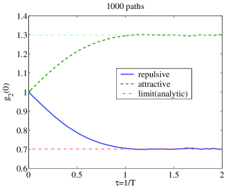
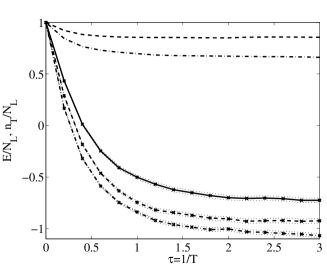
Figure 3: Hubbard models vs inverse temperature $\tau$. Left graph shows the second-order correlation function $g_{2}(0)=\left\langle\widehat{n}_{jj+}\widehat{n}_{jj-}\right\rangle/\left\langle\widehat{n}_{jj+}\right\rangle\left\langle\widehat{n}_{jj-}\right\rangle$ for a $100$-site 1D lattice at half-filling. $|U|=2$ and $t=1$. The right graph shows a $16\times 16$ 2D lattice for chemical potentials $\mu=2$ (solid), $\mu=1$ (dashed) and $\mu=0$ (dot-dashed). Curves without crosses give the number of particles per site for $\mu=1$ (dashed) and $\mu=0$ (dot-dashed). $U=4$, $t=1$, and 50 paths initially.

6 Summary

We have reviewed some recent theoretical developments for ultra-cold fermionic atoms in an optical lattice.

For the case of the Mott metal-insulator (MMIT) transition in one dimension, at zero temperature, we give a universal phase diagram based on the exact 1D solutions, and valid in the LDA limit of large traps. A crucial experimental signature was predicted, namely a strong frequency dip at the filling factor corresponding to the onset of the MMIT at the trap centre.

More generally, a novel exact technique for general dynamic and static Fermi calculations was presented. This can be used to calculate correlations of strongly-correlated fermions at any temperature - and for Hubbard models in any dimension. This is therefore a solution to the long-standing Fermi sign problem in the Hubbard model.

References

- [1] R. H. Wynar, R. S. Freeland, D. J. Han, C. Ryu, and D. J. Heinzen, Science 287, 1016 (2000).
- [2] E. A. Donley et al., Nature 417, 529 (2002).
- [3] P. D. Drummond, K. V. Kheruntsyan, and H. He, Phys. Rev. Lett. 81, 3055 (1998); K. V. Kheruntsyan and P. D. Drummond, Phys. Rev. A 61, 063816 (2000).
- [4] M. Holland et al., Phys. Rev. Lett. 87, 120406 (2001); S. J. J. M. F. Kokkelmans et al., Phys. Rev. A 65, 053617 (2002); R. A. Duine and H. T. C. Stoof, Phys. Rev. Lett. 91, 150405 (2003); P. D. Drummond and K. V. Kheruntsyan, Phys. Rev. A 70, 033609 (2004).
- [5] J. Herbig et al., Science 301, 1510 (2003); K. Xu., T. Mukaiyama et al., Phys. Rev. Lett. 91, 210402 (2003); S. Dürr et al., ibid. 92, 020406 (2004).
- [6] D. S. Petrov, C. Salomon, and G. V. Shlyapnikov, Phys. Rev. Lett. 93, 090404 (2004).
- [7] C. A. Regal et al., Nature 424, 47 (2003); K. E. Strecker et al., Phys. Rev. Lett. 91, 080406 (2003); K. J. Cubizolles et al., ibid. 91, 240401 (2003); S. Jochim et al., ibid. 91, 240402 (2003).
- [8] M. Greiner et al., Nature 426, 537 (2003); M. W. Zweirlein et al., Phys. Rev. Lett. 91, 250401 (2003).
- [9] C. A. Regal, M. Greiner, and D. S. Jin, Phys. Rev. Lett. 92, 040403 (2004); M. Bartenstein et al., ibid. 120401 (2004); M. W. Zwierlin et al., ibid. 120403 (2004).
- [10] M. Bartenstein et al., Phys. Rev. Lett. 92, 130403 (2004); J. Kinst et al., ibid. 150402 (2004); C. Chin et al., Science 305, 1128 (2004); J. Kinst et al., Science Express (27 Jan 2005).
- [11] D. Jaksch, C. Bruder, J. I. Cirac, C. W. Gardiner, and P. Zoller, Phys. Rev. Lett. 81, 3108-3111 (1998).
- [12] M. Greiner et al., Nature (London), 415, 39 (2002); B. Paredes et al., ibid. 429, 277 (2004).
- [13] A. Recati, P. O. Fedichev, W. Zwerger, and P. Zoller, Phys. Rev. Lett. 90, 020401 (2003).
- [14] L. Pezze et al., Phys. Rev. Lett. 93, 120401 (2004), M. Köhl, H. Moritz, T. Stöferle, K. Günter, and T. Esslinger, Phys. Rev. Lett. 94, 080403 (2005).
- [15] E. H. Lieb and F. Y. Wu, Phys. Rev. Lett. 20, 1445 (1968).
- [16] M. Rigol, A. Muramatsu, G. G. Batrouni and R. T. Scalettar, Phys. Rev. Lett. 91, 130403 (2003).
- [17] Xia-Ji Liu, Peter D. Drummond, and Hui Hu, Phys. Rev. Lett. 94, 136406 (2005).
- [18] R. Combescot and X. Leyronas, Phys. Rev. Lett. 89, 190405 (2002).
- [19] D. M. Ceperley, Rev. Mod. Phys. 71, 438 (1999); W. von der Linden, Phys. Rep. 220, 53 (1992); R. R. dos Santos, Brazilian Journal of Physics 33, 36 (2003).
- [20] J. F. Corney and P. D. Drummond, Phys. Rev. Lett. 93, 260401 (2004).
- [21] P. Deuar and P. D. Drummond, Phys. Rev. A 66, 033812 (2002); P. D. Drummond, P. Deuar, and K. V. Kheruntsyan, Phys. Rev. Lett. 92, 040405 (2004); M. R. Dowling, P. D. Drummond, M. J. Davis, and P. Deuar, Phys. Rev. Lett. 94, 130401 (2005).
- [22] J. F. Corney and P. D. Drummond, cond-mat/0411712.
- [23] J. F. Corney and P. D. Drummond, Phys. Rev. A 68, 063822 (2003).