$d=3$ Anisotropic and $d=2$ $tJ$ Models: Phase Diagrams, Thermodynamic Properties, and Chemical Potential Shift

Abstract

The anisotropic $d=3$  $tJ$ model is studied by renormalization-group theory, yielding the evolution of the system as interplane coupling is varied from the isotropic three-dimensional to quasi-two-dimensional regimes. Finite-temperature phase diagrams, chemical potential shifts, and in-plane and interplane kinetic energies and antiferromagnetic correlations are calculated for the entire range of electron densities. We find that the novel $\tau$ phase, seen in earlier studies of the isotropic $d=3$   $tJ$ model, persists even for strong anisotropy. While the $\tau$ phase appears at low temperatures at $30-35\%$ hole doping away from $\langle n_{i}\rangle=1$, at smaller hole dopings we see a complex lamellar structure of antiferromagnetic and disordered regions, with a suppressed chemical potential shift, a possible marker of incommensurate ordering in the form of microscopic stripes. An investigation of the renormalization-group flows for the isotropic two-dimensional $tJ$ model also shows a clear pre-signature of the $\tau$ phase, which in fact appears with finite transition temperatures upon addition of the smallest interplane coupling.

PACS numbers: 74.72.-h, 71.10.Fd, 05.30.Fk, 74.25.Dw

I Introduction

The anisotropic nature of high-$T_{c}$ materials, where groups of one or more CuO₂ planes are weakly coupled through block layers that act as charge reservoirs, has led to intense theoretical focus on two-dimensional models of electron conduction.ADagotto However, a full understanding of the cuprates will require taking into account physics along the third dimension. Crucial aspects of the phase diagram, like the finite value of the Néel temperature, depend on interplanar coupling AImada , and going beyond two dimensions is also necessary to explain the behavior of $T_{c}$ as the number of CuO₂ layers per unit cell is increased AChakravarty . Moreover, given the recent debate over the adequacy of the two-dimensional $tJ$ model as a description of high-$T_{c}$ superconductivity PryadkoKivelsonZachar ; KoretsuneOgata ; PutikkaLuchini ; Su , a resolution of the issue might be found by turning to highly anisotropic three-dimensional models Su .

As a simplified description of strongly correlated electrons in an anisotropic system, we look at the $tJ$ model on a cubic lattice with uniform interaction strengths in the $xy$ planes, and a weaker interaction in the $z$ direction. To obtain a finite-temperature phase diagram for the entire range of electron densities, we extend to anisotropic systems the renormalization-group approach that has been applied successfully in earlier studies of both $tJ$ and Hubbard models as isotropic $d=3$ systems.AFalicovBerkerT ; AFalicovBerker ; AHinczBerker1 ; AHinczBerker2 For the $d=3$ isotropic $tJ$ model, this approach has yielded an interesting phase diagram with antiferromagnetism near $\langle n_{i}\rangle=1$ and a new low-temperature “$\tau$” phase for 33-37% hole doping. Within this $\tau$ phase, the magnitude of the electron hopping strength in the Hamiltonian tends to infinity as the system is repeatedly rescaled.AFalicovBerker The calculated superfluid weight shows a marked peak in the $\tau$ phase, and both the temperature profile of the superfluid weight and the density of free carriers with hole doping is reminiscent of experimental results in cuprates.AHinczBerker2 Given these apparent links with cuprate physics, the next logical step is to ask whether the $\tau$ phase is present in the strongly anisotropic regime, which is the one directly relevant to experiments.

The extension of the position-space renormalization-group method to spatial anisotropy has recently been demonstrated with $d=3$ Ising, XY magnetic and percolation systems.AErbasTuncerYucesoyBerker We apply a similar anisotropic generalization to the electronic conduction model and find the evolution of the phase diagram from the isotropic $d=3$ to the quasi $d=2$ cases. While transition temperatures become lower, the $\tau$ phase does continue to exist even for very weak interplanar coupling. The density range of the $\tau$ phase remains stable as anisotropy is increased, while for 5-30% hole doping an intricate structure of antiferromagnetic and disordered phases develops, a possible indicator of underlying incommensurate order, manifested through the formation of microscopic stripes. Consistent with this interpretation, our system in this density range shows a characteristic “pinning” of the chemical potential with hole doping.

Lastly, we turn from the $d=3$ anisotropic case to the $d=2$ $tJ$ model, where earlier studies  AFalicovBerkerT ; AFalicovBerker have found no $\tau$ phase (but have elucidated the occurrence/non-occurrence of phase separation). Nevertheless, by looking at the low-temperature behavior of the renormalization-group flows, we find a compelling pre-signature of the $\tau$ phase even in $d=2$, at exactly the density range where the $\tau$ phase appears when the slightest interplanar coupling is added to the system.

II Anisotropic $tJ$ Hamiltonian

We consider the $tJ$ Hamiltonian on a cubic lattice with different interaction strenghts for nearest neighbors lying in the $xy$ plane or along the $z$ direction (respectively denoted by $\langle ij\rangle_{xy}$ and $\langle ij\rangle_{z}$):

$$\begin{split}H&=P\left[\tilde{t}_{xy}\sum_{\langle ij\rangle_{xy},\sigma}\left(c^{\dagger}_{i\sigma}c_{j\sigma}+c^{\dagger}_{j\sigma}c_{i\sigma}\right)\right.\\ &\qquad+\tilde{t}_{z}\sum_{\langle ij\rangle_{z},\sigma}\left(c^{\dagger}_{i\sigma}c_{j\sigma}+c^{\dagger}_{j\sigma}c_{i\sigma}\right)\\ &\qquad+\tilde{J}_{xy}\sum_{\langle ij\rangle_{xy}}\mathbf{S}_{i}\cdot\mathbf{S}_{j}+\tilde{J}_{z}\sum_{\langle ij\rangle_{z}}\mathbf{S}_{i}\cdot\mathbf{S}_{j}\\ &\qquad\left.-\tilde{V}_{xy}\sum_{\langle ij\rangle_{xy}}n_{i}n_{j}-\tilde{V}_{z}\sum_{\langle ij\rangle_{z}}n_{i}n_{j}-\tilde{\mu}\sum_{i}n_{i}\right]P\,.\end{split}$$ (1)

Here $c^{\dagger}_{i\sigma}$ and $c_{i\sigma}$ are creation and annihilation operators, obeying anticommutation rules, for an electron with spin $\sigma=\>\uparrow$ or $\downarrow$ at lattice site $i$, $n_{i\sigma}=c^{\dagger}_{i\sigma}c_{i\sigma}$, $n_{i}=n_{i\uparrow}+n_{i\downarrow}$ are the number operators, and $\mathbf{S}_{i}=\frac{1}{2}\sum_{\sigma\sigma^{\prime}}c^{\dagger}_{i\sigma}\mathbf{s}_{\sigma\sigma^{\prime}}c_{i\sigma^{\prime}}$ is the single-site spin operator, with $\mathbf{s}$ the vector of Pauli spin matrices. The entire Hamiltonian is sandwiched between projection operators $P=\prod_{i}(1-n_{i\downarrow}n_{i\uparrow})$, which project out states with doubly-occupied sites. The standard, isotropic $tJ$ Hamiltonian obtains when $\tilde{t}_{xy}=\tilde{t}_{z}$, $\tilde{J}_{xy}=\tilde{J}_{z}$, $\tilde{V}_{xy}=\tilde{V}_{z}$, and $\tilde{V}_{xy}/\tilde{J}_{xy}=\tilde{V}_{z}/\tilde{J}_{z}=1/4$.

For simplicity, we rewrite Eq. (1) using dimensionless interaction constants, and rearrange the $\tilde{\mu}$ chemical potential term to group the Hamiltonian into summations over the $xy$ and $z$ bonds:

$$\begin{split}-\beta H=&\sum_{\langle ij\rangle_{xy}}P\biggl{[}-t_{xy}\sum_{\sigma}\left(c^{\dagger}_{i\sigma}c_{j\sigma}+c^{\dagger}_{j\sigma}c_{i\sigma}\right)\\ &\qquad-J_{xy}\mathbf{S}_{i}\cdot\mathbf{S}_{j}+V_{xy}n_{i}n_{j}+\mu(n_{i}+n_{j})\biggr{]}P\\ +&\sum_{\langle ij\rangle_{z}}P\biggl{[}-t_{z}\sum_{\sigma}\left(c^{\dagger}_{i\sigma}c_{j\sigma}+c^{\dagger}_{j\sigma}c_{i\sigma}\right)\\ &\qquad-J_{z}\mathbf{S}_{i}\cdot\mathbf{S}_{j}+V_{z}n_{i}n_{j}+\mu(n_{i}+n_{j})\biggr{]}P\\ \equiv&\sum_{\langle ij\rangle_{xy}}\{-\beta H_{xy}(i,j)\}+\sum_{\langle ij\rangle_{z}}\{-\beta H_{z}(i,j)\}\,.\end{split}$$ (2)

Here $\beta=1/k_{B}T$, so that the interaction constants are related by $t_{xy}=\beta\tilde{t}_{xy}$, $t_{z}=\beta\tilde{t}_{z}$, $J_{xy}=\beta\tilde{J}_{xy}$, $J_{z}=\beta\tilde{J}_{z}$, $V_{xy}=\beta\tilde{V}_{xy}$, $V_{z}=\beta\tilde{V}_{z}$, and $\mu=\beta\tilde{\mu}/6$.

III Renormalization-Group Theory

III.1 Isotropic Transformation and Anisotropic Expectations

Since the isotropic model is a special case of Eq. (1), let us briefly outline the main steps in effecting the renormalization equations of earlier, isotropic studies AFalicovBerker ; AFalicovBerkerT ; AHinczBerker2 . We begin by setting up a decimation transformation for a one-dimensional $tJ$ chain, finding a thermodynamically equivalent Hamiltonian by tracing over the degrees of freedom at every other lattice site. With the vector $\mathbf{K}$ whose elements are the interaction constants in the Hamiltonian, the decimation can be expressed as a mapping of the original $d=1$ system onto a new system with interaction constants

$$\mathbf{K}^{\prime}=\mathbf{R}(\mathbf{K})\,.$$ (3)

The Migdal-Kadanoff AMigdal ; AKadanoff procedure has been remarkably successful, for systems both classical and quantum, in extending this transformation to $d>1$ (for an overview, see  AHinczBerker1 ). In this procedure, a subset of the nearest-neighbor interactions in the lattice are ignored, leaving behind a new $d$-dimensional hypercubic lattice where each point is connected to its neighbor by two consecutive nearest-neighbor segments of the original lattice. The decimation described above is applied to the middle site between the two consecutive segments, giving the renormalized nearest-neighbor couplings for the points forming the new lattice. We compensate for the interactions that are ignored in the original lattice by multiplying the interactions after the decimation by $b^{d-1}$, where $b=2$ is the length rescaling factor. Thus for $d>1$ the renormalization-group transformation of Eq. (3) generalizes to

$$\mathbf{K}^{\prime}=b^{d-1}\mathbf{R}(\mathbf{K}),$$ (4)

which, through flows in a four-dimensional Hamiltonian space (for the Hubbard model, 10-dimensional Hamiltonian space AHinczBerker1 ), yields a rich array of physical phenomena.

With the anisotropic $tJ$ Hamiltonian on a cubic lattice (Eq. (1)), there are two intercoupled sets of interaction constants, $\mathbf{K}_{xy}$ and $\mathbf{K}_{z}$, and further development of the transformation is needed. However, there are three particular instances where the transformation in Eq. (4) is directly applicable. When $\mathbf{K}_{xy}=\mathbf{K}_{z}$, we have the $d=3$ isotropic case, so the appropriate renormalization-group equations are

$$\mathbf{K}^{\prime}_{xy}=4\,\mathbf{R}(\mathbf{K}_{xy})\,,\qquad\mathbf{K}^{\prime}_{z}=4\,\mathbf{R}(\mathbf{K}_{z})\,.$$ (5)

When $\mathbf{K}_{xy}\neq 0$ and $\mathbf{K}_{z}=0$, we have a system of decoupled isotropic $d=2$ planes, and the transformation is given by

$$\mathbf{K}^{\prime}_{xy}=2\,\mathbf{R}(\mathbf{K}_{xy})\,,\qquad\mathbf{K}^{\prime}_{z}=0\,.$$ (6)

Similarly, when $\mathbf{K}_{xy}=0$ and $\mathbf{K}_{z}\neq 0$, we have decoupled $d=1$ chains, and

$$\mathbf{K}^{\prime}_{xy}=0\,,\qquad\mathbf{K}^{\prime}_{z}=\mathbf{R}(\mathbf{K}_{z})\,.$$ (7)

The renormalization-group transformation for the anisotropic model described in the following sections recovers the correct results, Eqs.(5)-(7), for these three cases.

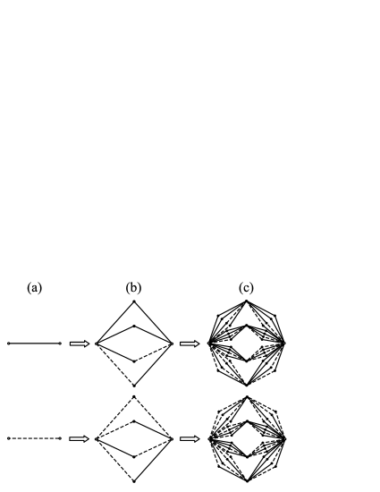
Figure 1: Construction of the hierarchical model in Section II.B. Solid lines correspond to $xy$ bonds, while dashed lines correspond to $z$ bonds.

III.2 Hierarchical Lattice Model for Anisotropy

A one-to-one correspondance exists between Migdal-Kadanoff and other approximate renormalization-group transformations on the one hand, and exact renormalization-group transformations of corresponding hierarchical lattices on the other hand, through the sharing of identical recursion relations.ABerkerOstlund ; AGriffithsKaufman ; Kaufman2 The correspondance guarantees the fulfilment of general physical preconditions on the results of approximate renormalization-group transformations, since the latter are thus “physically realizable”.ABerkerOstlund This correspondance has recently been exploited to develop renormalization-group transformations for spatially anisotropic Ising, XY magnetic and percolation systems.AErbasTuncerYucesoyBerker Similarly, to derive an approximate renormalization-group transformation for the anisotropic $tJ$ Hamiltonian, consider the nonuniform hierarchical model depicted in Fig. 1. The two types of bonds in the lattice, corresponding to $xy$ and $z$ bonds, are drawn with solid and dashed lines respectively. The hierarchical model is constructed by replacing each single bond of a given type with the connected cluster of bonds shown in Fig. 1(b), and repeating this step an arbitrary number of times. Fig. 1(c) shows the next stage in the construction for the two graphs in column (b). The renormalization-group transformation on this hierarchical lattice consists of decimating over the four inner sites in each cluster, to generate a renormalized interaction between the two outer sites, thus reversing the construction process, going from the graphs in column (b) of Fig. 1 to those in column (a). This renormalization-group transformation has the desired feature that in all three of the cases described above, it reproduces the various isotropic recursion relations of Eqs. (5)-(7).

III.3 Renormalization-Group Equations for Anisotropic System

The hierarchical lattice can be subdivided into individual clusters of bonds shown in Fig. 1(b). We label these two types of clusters the “$xy$ cluster” (Fig. 1(b) top) and the “$z$ cluster” (Fig. 1(b) bottom). The sum over $\langle ij\rangle_{\text{$xy$ clus}}$ denotes a sum over the outer sites of all the $xy$ clusters, and analogously $\langle ij\rangle_{\text{$z$ clus}}$ denotes a sum over the outer sites of all $z$ clusters. For a given cluster with outer sites $ij$, the associated inner sites are labeled $k^{(ij)}_{1},\ldots,k^{(ij)}_{4}$. Then the $tJ$ Hamiltonian on the anisotropic lattice has the form

$$\begin{split}-\beta H&=\sum_{\langle ij\rangle_{\text{$xy$ clus}}}\Bigl{[}-\beta H_{xy}(i,k^{(ij)}_{1})-\beta H_{xy}(k^{(ij)}_{1},j)-\beta H_{xy}(i,k^{(ij)}_{2})-\beta H_{xy}(k^{(ij)}_{2},j)\\ &\qquad-\beta H_{xy}(i,k^{(ij)}_{3})-\beta H_{z}(k^{(ij)}_{3},j)-\beta H_{z}(i,k^{(ij)}_{4})-\beta H_{xy}(k^{(ij)}_{4},j)\Bigr{]}\\ &+\sum_{\langle ij\rangle_{\text{$z$ clus}}}\Bigl{[}-\beta H_{z}(i,k^{(ij)}_{1})-\beta H_{z}(k^{(ij)}_{1},j)-\beta H_{z}(i,k^{(ij)}_{2})-\beta H_{xy}(k^{(ij)}_{2},j)\\ &\qquad-\beta H_{xy}(i,k^{(ij)}_{3})-\beta H_{z}(k^{(ij)}_{3},j)-\beta H_{z}(i,k^{(ij)}_{4})-\beta H_{xy}(k^{(ij)}_{4},j)\Bigr{]}\,.\end{split}$$ (8)

The renormalization-group transformation consists of finding a thermodynamically equivalent Hamiltonian $-\beta^{\prime}H^{\prime}$ that involves only the outer sites of each cluster. Since we are dealing with a quantum system, the non-commutation of the operators in the Hamiltonian means that this decimation, tracing over the degrees of freedom at the $k$ sites, can only be carried out approximately ASuzTak ; ATakSuz :

$$\begin{split}\text{Tr}_{\text{$k$ sites}}\,e^{-\beta H}&\simeq\prod_{\langle ij\rangle_{\text{$xy$ clus}}}\Bigl{[}\text{Tr}_{k^{(ij)}_{1}}\,e^{-\beta H_{xy}(i,k^{(ij)}_{1})-\beta H_{xy}(k^{(ij)}_{1},j)}\,\text{Tr}_{k^{(ij)}_{2}}\,e^{-\beta H_{xy}(i,k^{(ij)}_{2})-\beta H_{xy}(k^{(ij)}_{2},j)}\\ &\qquad\qquad\text{Tr}_{k^{(ij)}_{3}}\,e^{-\beta H_{xy}(i,k^{(ij)}_{3})-\beta H_{z}(k^{(ij)}_{3},j)}\,\text{Tr}_{k^{(ij)}_{4}}\,e^{-\beta H_{z}(i,k^{(ij)}_{4})-\beta H_{xy}(k^{(ij)}_{4},j)}\Bigr{]}\\ &\quad\cdot\prod_{\langle ij\rangle_{\text{$z$ clus}}}\Bigl{[}\text{Tr}_{k^{(ij)}_{1}}\,e^{-\beta H_{z}(i,k^{(ij)}_{1})-\beta H_{z}(k^{(ij)}_{1},j)}\,\text{Tr}_{k^{(ij)}_{2}}\,e^{-\beta H_{z}(i,k^{(ij)}_{2})-\beta H_{xy}(k^{(ij)}_{2},j)}\\ &\qquad\qquad\text{Tr}_{k^{(ij)}_{3}}\,e^{-\beta H_{xy}(i,k^{(ij)}_{3})-\beta H_{z}(k^{(ij)}_{3},j)}\,\text{Tr}_{k^{(ij)}_{4}}\,e^{-\beta H_{z}(i,k^{(ij)}_{4})-\beta H_{xy}(k^{(ij)}_{4},j)}\Bigr{]}\\ &=\prod_{\langle ij\rangle_{\text{$xy$ clus}}}\Bigl{[}e^{-\beta^{\prime}H^{\prime}_{xy,xy}(i,j)}e^{-\beta^{\prime}H^{\prime}_{xy,xy}(i,j)}e^{-\beta^{\prime}H^{\prime}_{xy,z}(i,j)}e^{-\beta^{\prime}H^{\prime}_{z,xy}(i,j)}\Bigr{]}\\ &\quad\cdot\prod_{\langle ij\rangle_{\text{$z$ clus}}}\Bigl{[}e^{-\beta^{\prime}H^{\prime}_{z,z}(i,j)}e^{-\beta^{\prime}H^{\prime}_{xy,z}(i,j)}e^{-\beta^{\prime}H^{\prime}_{z,xy}(i,j)}e^{-\beta^{\prime}H^{\prime}_{z,xy}(i,j)}\Bigr{]}\\ &\simeq e^{\sum_{\langle ij\rangle_{\text{$xy$ clus}}}\left[-2\beta^{\prime}H^{\prime}_{xy,xy}(i,j)-\beta^{\prime}H^{\prime}_{xy,z}(i,j)-\beta^{\prime}H^{\prime}_{z,xy}(i,j)\right]+\sum_{\langle ij\rangle_{\text{$z$ clus}}}\left[-\beta^{\prime}H^{\prime}_{z,z}(i,j)-\beta^{\prime}H^{\prime}_{xy,z}(i,j)-2\beta^{\prime}H^{\prime}_{z,xy}(i,j)\right]}\\ &=e^{\sum_{\langle ij\rangle_{\text{$xy$ clus}}}\left[-\beta^{\prime}H_{xy}^{\prime}(i,j)\right]+\sum_{\langle ij\rangle_{\text{$z$ clus}}}\left[-\beta^{\prime}H^{\prime}_{z}(i,j)\right]}\ =e^{-\beta^{\prime}H^{\prime}}\,.\end{split}$$ (9)

Here $-\beta^{\prime}H^{\prime}_{A,B}(i,j)$, where $A$, $B$ can each be either $xy$ or $z$, is

$$e^{-\beta^{\prime}H^{\prime}_{A,B}(i,j)}=\text{Tr}_{k}\,e^{-\beta H_{A}(i,k)-\beta H_{B}(k,j)}\,.$$ (10)

In the two approximate steps, marked by $\simeq$ in Eq. (9), we ignore the non-commutation of operators outside three-site segments of the unrenormalized system. (On the other hand, anticommutation rules are correctly accounted for within the three-site segments, at all successive length scales in the iterations of the renormalization-group transformation.) These two steps involve the same approximation but in opposite directions, which gives some mutual compensation. This approach has been shown to successfully predict finite-temperature behavior in earlier studies ASuzTak ; ATakSuz .

Derivation of the renormalization-group equations involves extracting the algebraic form of the operators $-\beta^{\prime}H^{\prime}_{A,B}(i,j)$ from Eq. (10). Since $e^{-\beta^{\prime}H^{\prime}_{A,B}(i,j)}$ and $e^{-\beta H_{A}(i,k)-\beta H_{B}(k,j)}$ act on the space of two-site and three-site states respectively, Eq. (10) can be rewritten in terms of matrix elements as

$$\begin{split}&\langle u_{i}v_{j}|e^{-\beta^{\prime}H^{\prime}_{A,B}(i,j)}|\bar{u}_{i}\bar{v}_{j}\rangle\\ &\qquad=\sum_{w_{k}}\langle u_{i}w_{k}v_{j}|e^{-\beta H_{A}(i,k)-\beta H_{B}(k,j)}|\bar{u}_{i}w_{k}\bar{v}_{j}\rangle\,,\end{split}$$ (11)

where $u_{i},w_{k},v_{j},\bar{u}_{i},\bar{v}_{j}$ are single-site state variables. Eq.(11) is the contraction of a $27\times 27$ matrix on the right into a $9\times 9$ matrix on the left. We block-diagonalize the left and right sides of Eq.(11) by choosing basis states which are the eigenstates of total particle number, total spin magnitude, total spin $z$-component, and parity. We denote the set of 9 two-site eigenstates by $\{|\phi_{p}\rangle\}$ and the set of 27 three-site eigenstates by $\{|\psi_{q}\rangle\}$, and list them in Tables I and II. Eq.(11) is rewritten as

$$\begin{split}&\langle\phi_{p}|e^{-\beta^{\prime}H_{A,B}^{\prime}(i,j)}|\phi_{\bar{p}}\rangle=\\ &\sum_{\begin{subarray}{c}u,v,\bar{u},\\ \bar{v},w\end{subarray}}\sum_{\begin{subarray}{c}q,\bar{q}\end{subarray}}\langle\phi_{p}|u_{i}v_{j}\rangle\langle u_{i}w_{k}v_{j}|\psi_{q}\rangle\\ &\quad\cdot\langle\psi_{q}|e^{-\beta H_{A}(i,k)-\beta H_{B}(k,j)}|\psi_{\bar{q}}\rangle\langle\psi_{\bar{q}}|\bar{u}_{i}w_{k}\bar{v}_{j}\rangle\langle\bar{u}_{i}\bar{v}_{j}|\phi_{\bar{p}}\rangle\>.\end{split}$$ (12)

Eq. (12) yields six independent elements for the matrix $\langle\phi_{p}|e^{-\beta^{\prime}H_{A,B}^{\prime}(i,j)}|\phi_{\bar{p}}\rangle$, labeled $\gamma_{p}$ as follows:

$$\begin{split}\gamma_{p}&\equiv\langle\phi_{p}|e^{-\beta^{\prime}H_{A,B}^{\prime}(i,j)}|\phi_{p}\rangle\quad\text{for}\>p=1,2,4,6,7,\\ \gamma_{0}&\equiv\langle\phi_{2}|e^{-\beta^{\prime}H_{A,B}^{\prime}(i,j)}|\phi_{4}\rangle\,.\end{split}$$ (13)

The number of $\gamma_{p}$ is also the number of interaction strengths that are independently fixed in the Hamiltonian $-\beta^{\prime}H_{A,B}^{\prime}(i,j)$, which consequently must have a more general form than the two-site Hamiltonians in Eq. (2). The generalized form of the pair Hamiltonian is

$$\begin{split}-\beta H(i,j)&=P\biggl{[}-t\sum_{\sigma}\left(c^{\dagger}_{i\sigma}c_{j\sigma}+c^{\dagger}_{j\sigma}c_{i\sigma}\right)\\ &\qquad-J\mathbf{S}_{i}\cdot\mathbf{S}_{j}+Vn_{i}n_{j}\\ &\qquad+\mu(n_{i}+n_{j})+\nu(n_{i}-n_{j})+G\biggr{]}P\end{split}$$ (14)

The new terms here are: $G$, the additive constant that appears in all renormalization-group calculations, does not affect the flows, but enters the determination of expectation values; and $\nu(n_{i}-n_{j})$, a staggered term arising from decimation across two consecutive bonds of different strengths. Provisions for handling the $\nu$ term will be described later in this section.

To calculate the $\gamma_{p}$, we determine the matrix elements of $-\beta H_{A}(i,k)-\beta H_{B}(k,j)$ in the three-site basis $\{\psi_{q}\}$. $-\beta H_{A}$ and $-\beta H_{B}$ have the form of Eq. (14), with interaction constants $\{t_{A},$ $J_{A},$ $V_{A},$ $\mu_{A},$ $\nu_{A},$ $G_{A}\}$ and $\{t_{B},$ $J_{B},$ $V_{B},$ $\mu_{B},$ $\nu_{B},$ $G_{B}\}$ respectively. The resulting matrix elements are listed in Table III. We exponentiate the matrix blocks to find the elements $\langle\psi_{q}|e^{-\beta H_{A}(i,k)-\beta H_{B}(k,j)}|\psi_{\bar{q}}\rangle$ which enter on the right-hand side of Eq. (12). In this way the $\gamma_{p}$ are obtained as functions of the interaction constants in the unrenormalized two-site Hamiltonians, $\gamma_{p}=\gamma_{p}(\{t_{A},J_{A},\ldots\},\{t_{B},J_{B},\ldots\})$.

$n$	$p$	$s$	$m_{s}$	Two-site basis states
$0$	$+$	$0$	$0$	$|\phi_{1}\rangle=|\circ\circ\rangle$
$1$	$+$	$1/2$	$1/2$	$|\phi_{2}\rangle=\frac{1}{\sqrt{2}}\{|\uparrow\circ\rangle+|\circ\uparrow\rangle\}$
$1$	$-$	$1/2$	$1/2$	$|\phi_{4}\rangle=\frac{1}{\sqrt{2}}\{|\uparrow\circ\rangle-|\circ\uparrow\rangle\}$
$2$	$-$	$0$	$0$	$|\phi_{6}\rangle=\frac{1}{\sqrt{2}}\{|\uparrow\downarrow\rangle-|\downarrow\uparrow\rangle\}$
$2$	$+$	$1$	$1$	$|\phi_{7}\rangle=|\uparrow\uparrow\rangle$
$2$	$+$	$1$	$0$	$|\phi_{9}\rangle=\frac{1}{\sqrt{2}}\{|\uparrow\downarrow\rangle+|\downarrow\uparrow\rangle\}$

Table I: The two-site basis states, with the corresponding particle number ($n$), parity ($p$), total spin ($s$), and total spin $z$-component ($m_{s}$) quantum numbers. The states $|\phi_{3}\rangle$, $|\phi_{5}\rangle$, and $|\phi_{8}\rangle$ are obtained by spin reversal from $|\phi_{2}\rangle$, $|\phi_{4}\rangle$, and $|\phi_{7}\rangle$, respectively.

$n$	$p$	$s$	$m_{s}$	Three-site basis states
$0$	$+$	$0$	$0$	$|\psi_{1}\rangle=|\circ\circ\,\circ\rangle$
$1$	$+$	$1/2$	$1/2$	$|\psi_{2}\rangle=|\circ\uparrow\circ\rangle,\>|\psi_{3}\rangle=\frac{1}{\sqrt{2}}\{|\uparrow\circ\,\circ\rangle+|\circ\,\circ\uparrow\rangle\}$
$1$	$-$	$1/2$	$1/2$	$|\psi_{6}\rangle=\frac{1}{\sqrt{2}}\{|\uparrow\circ\,\circ\rangle-|\circ\,\circ\uparrow\rangle\}$
$2$	$+$	$0$	$0$	$|\psi_{8}\rangle=\frac{1}{2}\{|\uparrow\downarrow\circ\rangle-|\downarrow\uparrow\circ\rangle-|\circ\uparrow\downarrow\rangle+|\circ\downarrow\uparrow\rangle\}$
$2$	$-$	$0$	$0$	$|\psi_{9}\rangle=\frac{1}{2}\{|\uparrow\downarrow\circ\rangle-|\downarrow\uparrow\circ\rangle+|\circ\uparrow\downarrow\rangle-|\circ\downarrow\uparrow\rangle\},$
				$|\psi_{10}\rangle=\frac{1}{\sqrt{2}}\{|\uparrow\circ\downarrow\rangle-|\downarrow\circ\uparrow\rangle\}$
$2$	$+$	$1$	$1$	$|\psi_{11}\rangle=|\uparrow\circ\uparrow\rangle,\>|\psi_{12}\rangle=\frac{1}{\sqrt{2}}\{|\uparrow\uparrow\circ\rangle+|\circ\uparrow\uparrow\rangle\}$
$2$	$+$	$1$	$0$	$|\psi_{13}\rangle=\frac{1}{2}\{|\uparrow\downarrow\circ\rangle+|\downarrow\uparrow\circ\rangle+|\circ\uparrow\downarrow\rangle+|\circ\downarrow\uparrow\rangle\},$
				$|\psi_{14}\rangle=\frac{1}{\sqrt{2}}\{|\uparrow\circ\downarrow\rangle+|\downarrow\circ\uparrow\rangle\}$
$2$	$-$	$1$	$1$	$|\psi_{17}\rangle=\frac{1}{\sqrt{2}}\{|\uparrow\uparrow\circ\rangle-|\circ\uparrow\uparrow\rangle\}$
$2$	$-$	$1$	$0$	$|\psi_{18}\rangle=\frac{1}{2}\{|\uparrow\downarrow\circ\rangle+|\downarrow\uparrow\circ\rangle-|\circ\uparrow\downarrow\rangle-|\circ\downarrow\uparrow\rangle\}$
$3$	$+$	$1/2$	$1/2$	$|\psi_{20}\rangle=\frac{1}{\sqrt{6}}\{2|\uparrow\downarrow\uparrow\rangle-|\uparrow\uparrow\downarrow\rangle-|\downarrow\uparrow\uparrow\rangle\}$
$3$	$-$	$1/2$	$1/2$	$|\psi_{22}\rangle=\frac{1}{\sqrt{2}}\{|\uparrow\uparrow\downarrow\rangle-|\downarrow\uparrow\uparrow\rangle\}$
$3$	$+$	$3/2$	$3/2$	$|\psi_{24}\rangle=|\uparrow\uparrow\uparrow\rangle$
$3$	$+$	$3/2$	$1/2$	$|\psi_{25}\rangle=\frac{1}{\sqrt{3}}\{|\uparrow\downarrow\uparrow\rangle+|\uparrow\uparrow\downarrow\rangle+|\downarrow\uparrow\uparrow\rangle\}$

Table II: The three-site basis states, with the corresponding particle number ($n$), parity ($p$), total spin ($s$), and total spin $z$-component ($m_{s}$) quantum numbers. The states $|\psi_{4-5}\rangle$, $|\psi_{7}\rangle$, $|\psi_{15-16}\rangle$, $|\psi_{19}\rangle$, $|\psi_{21}\rangle$, $|\psi_{23}\rangle$, $|\psi_{26-27}\rangle$ are obtained by spin reversal from $|\psi_{2-3}\rangle$, $|\psi_{6}\rangle$, $|\psi_{11-12}\rangle$, $|\psi_{17}\rangle$, $|\psi_{20}\rangle$, $|\psi_{22}\rangle$, $|\psi_{24-25}\rangle$, respectively.

$$\begin{array}[]{|c||c|}\hline\cr&\psi_{1}\\ \hline\cr\psi_{1}&0\\ \hline\cr\end{array}$$

$$\begin{array}[]{|c||c|c|c|}\hline\cr&\psi_{2}&\psi_{3}&\psi_{6}\\ \hline\cr\psi_{2}&\parbox{36.135pt}{$\mu_{A}+\mu_{B}-\nu_{A}+\nu_{B}$}&-\frac{1}{\sqrt{2}}(t_{A}+t_{B})&\frac{1}{\sqrt{2}}(t_{B}-t_{A})\\ \hline\cr\psi_{3}&-\frac{1}{\sqrt{2}}(t_{A}+t_{B})&\parbox{50.58878pt}{$\frac{1}{2}(\mu_{A}+\mu_{B}+\nu_{A}-\nu_{B})$}&\parbox{50.58878pt}{$\frac{1}{2}(\mu_{A}-\mu_{B}+\nu_{A}+\nu_{B})$}\\ \hline\cr\psi_{6}&\frac{1}{\sqrt{2}}(t_{B}-t_{A})&\parbox{50.58878pt}{$\frac{1}{2}(\mu_{A}-\mu_{B}+\nu_{A}+\nu_{B})$}&\parbox{50.58878pt}{$\frac{1}{2}(\mu_{A}+\mu_{B}+\nu_{A}-\nu_{B})$}\\ \hline\cr\end{array}$$

$$\begin{array}[]{|c||c|c|c|}\hline\cr&\psi_{8}&\psi_{9}&\psi_{10}\\ \hline\cr\psi_{8}&\parbox{65.04256pt}{$\frac{1}{2}(\frac{3}{4}J_{A}+\frac{3}{4}J_{B}+V_{A}+V_{B}+3\mu_{A}+3\mu_{B}-\nu_{A}+\nu_{B})$}&\parbox{65.04256pt}{$\frac{1}{2}(\frac{3}{4}J_{A}-\frac{3}{4}J_{B}+V_{A}-V_{B}+\mu_{A}-\mu_{B}+\nu_{A}+\nu_{B})$}&\frac{1}{\sqrt{2}}(t_{A}-t_{B})\\ \hline\cr\psi_{9}&\parbox{65.04256pt}{$\frac{1}{2}(\frac{3}{4}J_{A}-\frac{3}{4}J_{B}+V_{A}-V_{B}+\mu_{A}-\mu_{B}+\nu_{A}+\nu_{B})$}&\parbox{65.04256pt}{$\frac{1}{2}(\frac{3}{4}J_{A}+\frac{3}{4}J_{B}+V_{A}+V_{B}+3\mu_{A}+3\mu_{B}-\nu_{A}+\nu_{B})$}&-\frac{1}{\sqrt{2}}(t_{A}+t_{B})\\ \hline\cr\psi_{10}&\frac{1}{\sqrt{2}}(t_{A}-t_{B})&-\frac{1}{\sqrt{2}}(t_{A}+t_{B})&\parbox{36.135pt}{$\mu_{A}+\mu_{B}+\nu_{A}-\nu_{B}$}\\ \hline\cr\end{array}$$

$$\begin{array}[]{|c||c|c|c|}\hline\cr&\psi_{11}&\psi_{12}&\psi_{17}\\ \hline\cr\psi_{11}&\parbox{36.135pt}{$\mu_{A}+\mu_{B}+\nu_{A}-\nu_{B}$}&-\frac{1}{\sqrt{2}}(t_{A}+t_{B})&\frac{1}{\sqrt{2}}(t_{A}-t_{B})\\ \hline\cr\psi_{12}&-\frac{1}{\sqrt{2}}(t_{A}+t_{B})&\parbox{65.04256pt}{$\frac{1}{2}(-\frac{1}{4}J_{A}-\frac{1}{4}J_{B}+V_{A}+V_{B}+3\mu_{A}+3\mu_{B}-\nu_{A}+\nu_{B})$}&\parbox{65.04256pt}{$\frac{1}{2}(-\frac{1}{4}J_{A}+\frac{1}{4}J_{B}+V_{A}-V_{B}+\mu_{A}-\mu_{B}+\nu_{A}+\nu_{B})$}\\ \hline\cr\psi_{17}&\frac{1}{\sqrt{2}}(t_{A}-t_{B})&\parbox{65.04256pt}{$\frac{1}{2}(-\frac{1}{4}J_{A}+\frac{1}{4}J_{B}+V_{A}-V_{B}+\mu_{A}-\mu_{B}+\nu_{A}+\nu_{B})$}&\parbox{65.04256pt}{$\frac{1}{2}(-\frac{1}{4}J_{A}-\frac{1}{4}J_{B}+V_{A}+V_{B}+3\mu_{A}+3\mu_{B}-\nu_{A}+\nu_{B})$}\\ \hline\cr\end{array}$$

$$\begin{array}[]{|c||c|c|c|}\hline\cr&\psi_{13}&\psi_{14}&\psi_{18}\\ \hline\cr\psi_{13}&\parbox{65.04256pt}{$\frac{1}{2}(-\frac{1}{4}J_{A}-\frac{1}{4}J_{B}+V_{A}+V_{B}+3\mu_{A}+3\mu_{B}-\nu_{A}+\nu_{B})$}&-\frac{1}{\sqrt{2}}(t_{A}+t_{B})&\parbox{65.04256pt}{$\frac{1}{2}(-\frac{1}{4}J_{A}+\frac{1}{4}J_{B}+V_{A}-V_{B}+\mu_{A}-\mu_{B}+\nu_{A}+\nu_{B})$}\\ \hline\cr\psi_{14}&-\frac{1}{\sqrt{2}}(t_{A}+t_{B})&\parbox{36.135pt}{$\mu_{A}+\mu_{B}+\nu_{A}-\nu_{B}$}&\frac{1}{\sqrt{2}}(t_{A}-t_{B})\\ \hline\cr\psi_{18}&\parbox{65.04256pt}{$\frac{1}{2}(-\frac{1}{4}J_{A}+\frac{1}{4}J_{B}+V_{A}-V_{B}+\mu_{A}-\mu_{B}+\nu_{A}+\nu_{B})$}&\frac{1}{\sqrt{2}}(t_{A}-t_{B})&\parbox{65.04256pt}{$\frac{1}{2}(-\frac{1}{4}J_{A}-\frac{1}{4}J_{B}+V_{A}+V_{B}+3\mu_{A}+3\mu_{B}-\nu_{A}+\nu_{B})$}\\ \hline\cr\end{array}$$

$$\begin{array}[]{|c||c|c|}\hline\cr&\psi_{20}&\psi_{22}\\ \hline\cr\psi_{20}&\parbox{72.26999pt}{$\frac{1}{2}J_{A}+\frac{1}{2}J_{B}+V_{A}+V_{B}+2\mu_{A}+2\mu_{B}$}&\frac{\sqrt{3}}{4}(J_{B}-J_{A})\\ \hline\cr\psi_{22}&\frac{\sqrt{3}}{4}(J_{B}-J_{A})&\parbox{65.04256pt}{$V_{A}+V_{B}+2\mu_{A}+2\mu_{B}$}\\ \hline\cr\end{array}$$

$$\begin{array}[]{|c||c|}\hline\cr&\psi_{24}\\ \hline\cr\psi_{24}&\parbox{72.26999pt}{$-\frac{1}{4}J_{A}-\frac{1}{4}J_{B}+V_{A}+V_{B}+2\mu_{A}+2\mu_{B}$}\\ \hline\cr\end{array}\quad\begin{array}[]{|c||c|}\hline\cr&\psi_{25}\\ \hline\cr\psi_{25}&\parbox{72.26999pt}{$-\frac{1}{4}J_{A}-\frac{1}{4}J_{B}+V_{A}+V_{B}+2\mu_{A}+2\mu_{B}$}\\ \hline\cr\end{array}$$

Table III: Diagonal matrix blocks of the unrenormalized three-site Hamiltonian $-\beta H_{A}(i,k)-\beta H_{B}(k,j)$. The Hamiltonian being invariant under spin-reversal, the spin-flipped matrix elements are not shown. The additive constant contribution $G_{A}+G_{B}$, occurring at the diagonal terms, is also not shown.

$$\begin{array}[]{|c||c|c|c|c|c|c|}\hline\cr&\parbox{5.78172pt}{$\phi_{1}$}&\phi_{2}&\phi_{4}&\phi_{6}&\phi_{7}&\phi_{9}\\ \hline\cr\parbox{7.22743pt}{$\phi_{1}$}&\parbox{5.78172pt}{$G^{\prime}$}&\lx@intercol\hfil\hfil\lx@intercol\vrule\lx@intercol\\ \cline{1-4}\cr\parbox{7.22743pt}{$\phi_{2}$}&&\parbox{28.90755pt}{\centering$-t^{\prime}+\mu^{\prime}+G^{\prime}$\@add@centering}&\nu^{\prime}&\lx@intercol\hfil 0\hfil\lx@intercol\vrule\lx@intercol\\ \cline{1-1}\cr\cline{3-4}\cr\parbox{7.22743pt}{$\phi_{4}$}&\lx@intercol\hfil\hfil\lx@intercol\vrule\lx@intercol&\nu^{\prime}&\parbox{28.90755pt}{\centering$t^{\prime}+\mu^{\prime}+G^{\prime}$\@add@centering}&\lx@intercol\hfil\hfil\lx@intercol\vrule\lx@intercol\\ \cline{1-1}\cr\cline{3-5}\cr\parbox{7.22743pt}{$\phi_{6}$}&\lx@intercol\hfil\hfil\lx@intercol\vrule\lx@intercol&\lx@intercol\hfil\parbox{41.55502pt}{\centering$\frac{3}{4}J^{\prime}+V^{\prime}+2\mu^{\prime}+G^{\prime}$\@add@centering}\hfil\lx@intercol\vrule\lx@intercol&\lx@intercol\hfil\hfil\lx@intercol\vrule\lx@intercol\\ \cline{1-1}\cr\cline{5-6}\cr\parbox{7.22743pt}{$\phi_{7}$}&\lx@intercol\hfil 0\hfil\lx@intercol\vrule\lx@intercol&\lx@intercol\hfil\parbox{35.05098pt}{\centering$-\frac{1}{4}J^{\prime}+V^{\prime}+2\mu^{\prime}+G^{\prime}$\@add@centering}\hfil\lx@intercol\vrule\lx@intercol&\\ \cline{1-1}\cr\cline{6-7}\cr\parbox{7.22743pt}{$\phi_{9}$}&\lx@intercol\hfil\hfil\lx@intercol\vrule\lx@intercol&\parbox{35.05098pt}{\centering$-\frac{1}{4}J^{\prime}+V^{\prime}+2\mu^{\prime}+G^{\prime}$\@add@centering}\\ \hline\cr\end{array}$$

Table IV: Block-diagonal matrix of the renormalized two-site Hamiltonian $-\beta^{\prime}H^{\prime}(i,j)$. The Hamiltonian being invariant under spin-reversal, the spin-flipped matrix elements are not shown.

The matrix elements of $-\beta^{\prime}H_{A,B}^{\prime}(i,j)$ in the $\{\phi_{p}\}$ basis are shown in Table IV. Exponentiating this matrix, we solve for the renormalized interaction constants $(t^{\prime}$, $J^{\prime}$, $V^{\prime}$, $\mu^{\prime}$, $\nu^{\prime}$, $G^{\prime})$ in terms of the $\gamma_{p}$:

$$t^{\prime}=u,\qquad J^{\prime}=\ln\frac{\gamma_{6}}{\gamma_{7}},$$

$$V^{\prime}=\frac{1}{4}\left\{\ln(\gamma_{1}^{4}\gamma_{6}\gamma_{7}^{3})-8v\right\},\qquad\mu^{\prime}=v-\ln\gamma_{1},$$

$$\nu^{\prime}=\frac{2u\gamma_{0}}{\gamma_{4}-\gamma_{2}},\qquad G^{\prime}=\ln\gamma_{1},$$ (15)

where

$$v=\frac{1}{2}\ln\left(\gamma_{2}\gamma_{4}-\gamma_{0}^{2}\right)\,,$$

$$u=\frac{\gamma_{4}-\gamma_{2}}{\sqrt{\left(\gamma_{4}-\gamma_{2}\right)^{2}+4\gamma_{0}^{2}}}\cosh^{-1}\left(\frac{\gamma_{4}+\gamma_{2}}{2e^{v}}\right).$$

The renormalization-group transformation described by Eqs. (12)-(15) can be expressed as a mapping of a three-site Hamiltonian with bonds having interaction constants $\mathbf{K}_{A}=\{t_{A},J_{A},V_{A},\mu_{A},\nu_{A},G_{A}\}$ and $\mathbf{K}_{B}=\{t_{B},J_{B},V_{B},\mu_{B},\nu_{B},G_{B}\}$ onto a two-site Hamiltonian with interaction constants

$$\mathbf{K}^{\prime}=\mathbf{R}(\mathbf{K}_{A},\mathbf{K}_{B})\,.$$ (16)

When $\nu_{A}=\nu_{B}=0$, this mapping has the property that if $\mathbf{R}(\mathbf{K}_{A},\mathbf{K}_{B})=\{t^{\prime},J^{\prime},V^{\prime},\mu^{\prime},\nu^{\prime},G^{\prime}\}$, then $\mathbf{R}(\mathbf{K}_{B},\mathbf{K}_{A})$ gives the same result, except that the sign of $\nu^{\prime}$ is switched. So $\mathbf{R}(\mathbf{K}_{A},\mathbf{K}_{A})$ has a zero $\nu^{\prime}$ component when $\nu_{A}=0$.

¿From Eq. (9), the renormalized $xy$- and $z$-bond interaction constants are

$$\begin{split}\mathbf{K}^{\prime}_{xy}&=2\mathbf{R}(\mathbf{K}_{xy},\mathbf{K}_{xy})+\mathbf{R}(\mathbf{K}_{xy},\mathbf{K}_{z})+\mathbf{R}(\mathbf{K}_{z},\mathbf{K}_{xy})\,,\\ \mathbf{K}^{\prime}_{z}&=\mathbf{R}(\mathbf{K}_{z},\mathbf{K}_{z})+\mathbf{R}(\mathbf{K}_{xy},\mathbf{K}_{z})+2\mathbf{R}(\mathbf{K}_{z},\mathbf{K}_{xy})\,.\end{split}$$ (17)

The staggered $\nu^{\prime}$ term cancels out in $\mathbf{K}^{\prime}_{xy}$. In constructing the anisotropic hierarchical lattice, we could have used a graph in which the lowest two bonds in Fig. 1(b) are interchanged. Averaging over these two realizations,

$$\begin{split}\mathbf{K}^{\prime}_{z}&=\mathbf{R}(\mathbf{K}_{z},\mathbf{K}_{z})+\frac{3}{2}\mathbf{R}(\mathbf{K}_{xy},\mathbf{K}_{z})+\frac{3}{2}\mathbf{R}(\mathbf{K}_{z},\mathbf{K}_{xy})\,,\end{split}$$ (18)

the $\nu^{\prime}$ term cancels out in $\mathbf{K}^{\prime}_{z}$ as well.

IV Phase Diagrams and Expectation Values as a Function of Anisotropy

Thermodynamic properties of the system, including the global phase diagram and expectation values of operators occurring in the Hamiltonian, are obtained from the analysis of the renormalization-group flows ABOP . The initial conditions for the flows are the interaction constants in the original anisotropic $tJ$ Hamiltonian. For the numerical results presented below, we use the following initial form: $t_{xy}=t$, $t_{z}=\alpha_{t}t$, $J_{xy}=J$, $J_{z}=\alpha_{J}J$, $V_{xy}=J_{xy}/4$, $V_{z}=J_{z}/4$, where $0\leq\alpha_{t},\alpha_{J}\leq 1$. For the anisotropy parameters $\alpha_{t}$ and $\alpha_{J}$, we use $\alpha_{J}=\alpha_{t}^{2}$, as dictated from the derivation of the $tJ$ Hamiltonian from the large-$U$ limit of the Hubbard model AShankarSingh .

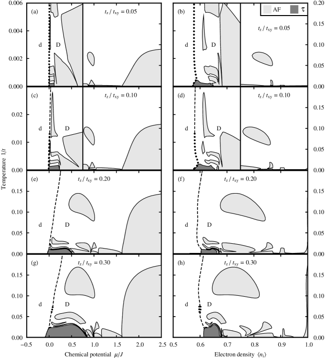
Figure 2: Phase diagrams of the anisotropic $tJ$ model with $J/t=0.444$ in temperature vs. chemical potential (first column) and temperature vs. electron density (second column). The degree of anisotropy varies from $t_{z}/t_{xy}=0.05$ in Fig. 2(a)-(b) to $t_{z}/t_{xy}=0.30$ in Fig. 2(g)-(h). Note the expanded temperature scales on the left panels of Fig. 2(a)-(d). The dense disordered (D), dilute disordered (d), antiferromagnetic (A), and $\tau$ phases are shown. The A and $\tau$ regions are colored light and dark gray respectively. Second-order phase transitions are drawn with full curves, first-order transitions with dotted curves. The unmarked areas within the dotted curves in the temperature vs. electron density figures are narrow coexistence regions between the two phases at either side. Dashed curves are not phase transitions, but disorder lines between the dense disordered and dilute disordered phases.

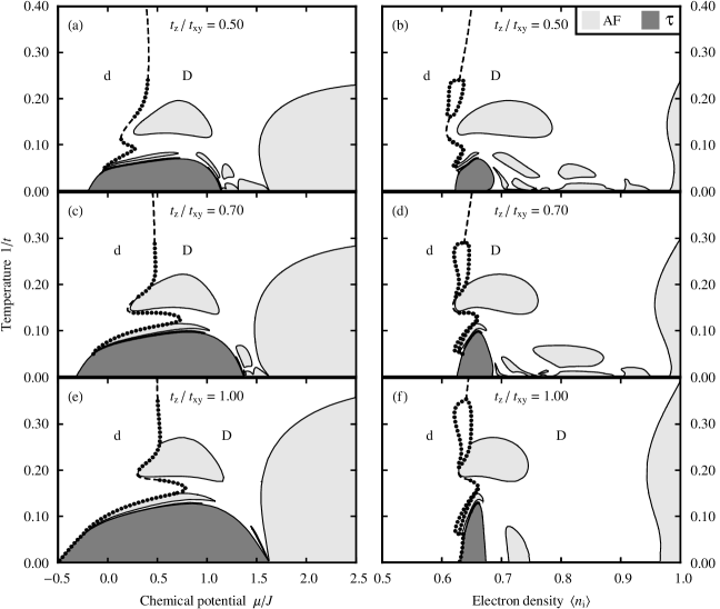
Figure 3: The continuation of the phase diagrams in Fig. 2 for $t_{z}/t_{xy}$ between 0.5 and 1.

Phase diagrams for the coupling $J/t=0.444$ and various values of $\alpha_{t}=t_{z}/t_{xy}$ are shown in Figs. 2 and 3. The temperature variable is $1/t$, and the diagrams are plotted both in terms of chemical potential $\mu/J$ and electron density $\langle n_{i}\rangle$. The phases in the diagrams are those found in earlier studies of the isotropic $d=3$ $tJ$ model AFalicovBerkerT ; AFalicovBerker , which can be consulted for a more detailed description. Here we summarize the salient features of the phases.

Each phase is associated with a completely stable fixed point (sink) of the renormalization-group flows, and thermodynamic densities calculated at the fixed point epitomize (and determine AHinczBerker2 , e.g., as seen in the results displayed in Fig. 4) characteristics of the entire phase. The results are shown in Table V. The dilute disordered (d) and dense disordered (D) phases have $\langle n_{i}\rangle=0$ and 1 at their respective phase sinks, so the electron densities in these phases are accordingly small in the one case and close to 1 in the other. Both phases lack long-range spin order, since $\langle\mathbf{S}_{i}\cdot\mathbf{S}_{j}\rangle=0$ at the sinks. On the other hand, the antiferromagnetic (A) phase has $\langle n_{i}\rangle=1$ and a nonzero nearest-neighbor spin-spin correlation $\langle\mathbf{S}_{i}\cdot\mathbf{S}_{j}\rangle=1/4$ at the phase sink. Since nearest-neighbor spins at the sink are distant members of the same sublattice in the unrenormalized system, this positive value for $\langle\mathbf{S}_{i}\cdot\mathbf{S}_{j}\rangle$ is expected, and leads to $\langle\mathbf{S}_{i}\cdot\mathbf{S}_{j}\rangle<0$ for nearest neighbors of the original system, as seen in the last row of Fig. 4.

Phase sink	Expectation values
	$-\sum_{\sigma}\langle c^{\dagger}_{i\sigma}c_{j\sigma}+c^{\dagger}_{j\sigma}c_{i\sigma}\rangle$	$\langle n_{i}\rangle$	$\langle\mathbf{S}_{i}\cdot\mathbf{S}_{j}\rangle$	$\langle n_{i}n_{j}\rangle$
d	0	0	0	0
D	0	1	0	1
A	0	1	$\frac{1}{4}$	1
$\tau$	$\frac{2}{3}$	$\frac{2}{3}$	$-\frac{1}{4}$	$\frac{1}{3}$

Table V: Expectation values at the phase-sink fixed points.

In the antiferromagnetic and the two disordered phases, the electron hopping strengths $t_{xy}$ and $t_{z}$ tend to zero after repeated rescalings. The system is either completely empty or filled in this limit, and the expectation value of the kinetic energy operator $\langle K\rangle\equiv-\sum_{\sigma}\langle c^{\dagger}_{i\sigma}c_{j\sigma}+c^{\dagger}_{j\sigma}c_{i\sigma}\rangle$ is zero at the sink. The $\boldsymbol{\tau}$ phase is interesting in contrast because the magnitudes of $t_{xy}$ and $t_{z}$ both tend to $\infty$, and we find partial filling, $\langle n_{i}\rangle=2/3$, and a nonzero kinetic energy $\langle K\rangle=2/3$ at the phase sink. It should be recalled that we have shown in a previous work AHinczBerker2 that the superfluid weight has a pronounced peak in the $\tau$ phase, there is evidence of a gap in the quasiparticle spectrum, and the free carrier density in the vicinity of the $\tau$ phase has properties seen experimentally in cuprates ABernhard2 ; APuchkov .

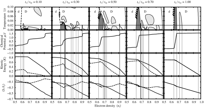
Figure 4: Thermodynamic properties along slices of the phase diagrams at the constant temperature $1/t=0.02$. The degree of anisotropy varies from $t_{z}/t_{xy}=0.10$ in the first column to $t_{z}/t_{xy}=1.00$ in the last column. The top row contains the temperature vs. electron density phase diagrams and a thin horizontal line marking the slice. The antiferromagnetic and $\tau$ phases are colored light and dark gray respectively. The rows below this show the chemical potential $\mu/J$, kinetic energy $\langle K\rangle=-\sum_{\sigma}\langle c^{\dagger}_{i\sigma}c_{j\sigma}+c^{\dagger}_{j\sigma}c_{i\sigma}\rangle$, and nearest-neighbor spin-spin correlation $\langle\mathbf{S}_{i}\cdot\mathbf{S}_{j}\rangle$. For the $\langle K\rangle$ and $\langle\mathbf{S}_{i}\cdot\mathbf{S}_{j}\rangle$ graphs, full curves denote results for nearest neighbors along the $xy$ plane, while dashed curves denote those for nearest neighbors along the $z$ direction. (In the $t_{z}/t_{xy}=1$ column, these two curves overlap.) Thin vertical lines mark the location of phase transitions.

Figs. 2 and 3 clearly demonstrate that the $\tau$ phase is not unique to the isotropic $d=3$ case, but exists at all values of $t_{z}/t_{xy}$, even persisting in the weak interplane coupling limit. Fig. 2 shows the evolution of the phase diagram in the strongly anisotropic regime, for $t_{z}/t_{xy}$ between 0.05 and 0.30, while Fig. 3 completes the evolution from $t_{z}/t_{xy}=0.5$ to the fully isotropic case where $t_{z}/t_{xy}=1$. The $\tau$ phase is present even for $t_{z}/t_{xy}=0.05$ and 0.10, but only at very low temperatures close to the d/D first-order phase transition that itself is distinct by its very narrow coexistence region. As the interplane coupling is increased, the $\tau$ phase transition temperatures also get larger, but the density range in which the phase occurs, namely $\langle n_{i}\rangle$ around 0.65, remains unchanged.

As expected, the antiferromagnetic transition temperatures also increase with the interplane coupling. The phase diagrams all share an antiferromagnetic region near $\langle n_{i}\rangle=1$, which is confined to $\langle n_{i}\rangle$ very close to 1 in the strongly anisotropic limit, but becomes more stable to hole doping as $t_{z}/t_{xy}$ gets larger. Away from $\langle n_{i}\rangle=1$, in the range of 5-35% hole doping, there are thin slivers and islands of antiferromagnetism separated by regions of the dense disordered phase. For $t_{z}/t_{xy}=1$, we see these mostly around the $\tau$ phase, but as anisotropy is introduced into the system, the structure of the antiferromagnetic regions becomes more complex, and spread out over a wider range of densities. The lamellar structure of A and D phases here potentially indicates an underlying incommensurate order AFalicovBerkerT . The physical significance of this possibility will be discussed below.

Further insight into the nature of the $\tau$ phase can be gained by looking at thermodynamic densities on a constant-temperature slice of the phase diagram. Fig. 4 plots the chemical potential $\mu/J$, kinetic energy $\langle K\rangle$, and nearest-neighbor spin-spin correlation $\langle\mathbf{S}_{i}\cdot\mathbf{S}_{j}\rangle$ at the temperature $1/t=0.02$ for several values of $t_{z}/t_{xy}$. Averages over the $xy$ bonds, $\langle\>\rangle_{xy}$ are drawn with full curves in the figure, and averages taken over the $z$ bonds, $\langle\>\rangle_{z}$ are drawn with dashed curves.

Consider first the kinetic energy expectation value $\langle K\rangle=-\sum_{\sigma}\langle c^{\dagger}_{i\sigma}c_{j\sigma}+c^{\dagger}_{j\sigma}c_{i\sigma}\rangle$. The $xy$ bond kinetic energy $\langle K\rangle_{xy}$ grows with hole doping until the density range where the $\tau$ phase occurs, and then levels off. This behavior is seen for the whole range of $t_{z}/t_{xy}$. We can compare our calculational result here with experimental results in cuprates, by relating the kinetic energy expectation value in the $tJ$ model to the density of free carriers as follows AHinczBerker2 . $\langle K\rangle$ and the total weight of $\sigma_{1}(\omega,T)$, the real part of the optical conductivity, satisfy the sum rule ATan

$$\int_{0}^{\infty}d\omega\,\sigma_{1}(\omega,T)=\frac{\pi e^{2}}{2}\langle K\rangle\,.$$ (19)

To understand this sum rule, we keep in mind that the $tJ$ Hamiltonian describes a one-band system, so cannot account for interband transitions. For real materials, the full conductivity sum rule has the form

$$\int_{0}^{\infty}d\omega\,\sigma_{1}(\omega,T)=\frac{\pi e^{2}n}{2m}\,,$$ (20)

where $n$ is the total density of electrons and $m$ is the free electron mass. The right-hand side of Eq. (20) is independent of electron-electron interactions, in contrast to the right-hand side of Eq. (19), where $\langle K\rangle$ varies with the interaction strengths in the Hamiltonian. The optical conductivity of actual materials incorporates both transitions within the conduction band and those to higher bands, while the $tJ$ model contains only the conduction band. We can look at Eq. (19) as a partial sum rule ABaeriswyl ; ATan , which reflects the spectral weight of the free carriers in the conduction band.

The experimental quantity we are interested in is the density of free carriers, which in actual materials is calculated from the low-frequency spectral weight AOrenstein ,

$$n_{\text{free}}(T)=\frac{2m_{b}}{\pi e^{2}}\int_{0}^{\omega_{0}}d\omega\,\sigma_{1}(\omega,T)\,,$$ (21)

where $m_{b}$ is the effective band mass of the electrons. For cuprates, the cut-off frequency is typically chosen around $\hbar\omega_{0}\approx 1$ eV so as to include only intraband transitions. In comparison with the $tJ$ model, we identify the right-hand side of Eq. (19) with

$$\frac{\pi e^{2}}{2}\langle K\rangle=\frac{\pi e^{2}n_{\text{free}}(T)}{2m_{b}}\,.$$ (22)

Puchkov et al.  APuchkov have studied the in-plane optical conductivity of a variety of cuprates, and found that the low-frequency spectral weight increases with doping until the doping level optimal for superconductivity is reached, and then remains approximately constant in the overdoped regime. This behavior of $n_{\text{free}}/m_{b}$ is qualitatively reproduced in our results for $\langle K\rangle_{xy}$.

As for $\langle K\rangle_{z}$, it is significantly reduced with increasing anisotropy, since interplane hopping is suppressed. $\langle K\rangle_{z}$ peaks in the $\tau$ phase, and decreases for larger dopings. This small peak in $\langle K\rangle_{z}$, which is most pronounced in the strongly anisotropic regime, is accompanied by an enhancement in the $\tau$ phase of the $z$-bond antiferromagnetic nearest-neighbor spin-spin correlation, $\langle\mathbf{S}_{i}\cdot\mathbf{S}_{j}\rangle_{z}$. For the $xy$ planes, $\langle\mathbf{S}_{i}\cdot\mathbf{S}_{j}\rangle_{xy}$ generally increases (i.e., becomes less negative) with hole doping from a large negative value near $\langle n_{i}\rangle=1$, as additional holes weaken the antiferromagnetic order. This increase becomes much less pronounced when the $\tau$ phase is reached, and $\langle\mathbf{S}_{i}\cdot\mathbf{S}_{j}\rangle_{xy}$ becomes nearly constant for large hole dopings in the strongly anisotropic limit. Rather than increasing with hole doping, $\langle\mathbf{S}_{i}\cdot\mathbf{S}_{j}\rangle_{z}$ shows the opposite behavior in the 10-35% doping range, decreasing and reaching a minimum within the $\tau$ phase.

The final aspect of the $\tau$ phase worth noting is the large change in chemical potential $\mu/J$ over the narrow density range where this phase occurs. This is in contrast to broad regions at smaller hole dopings where the chemical potential change is much shallower, and which correspond to those parts of the phase diagram where A and D alternate. We can see this directly in the phase diagram topology in Figs. 2 and 3, particularly for larger $t_{z}/t_{xy}$. The $\tau$ phase has a very wide extent in terms of chemical potential, but becomes very narrow in the corresponding electron density diagram. The converse is true for the complex lamellar structure of A and D phases sandwiched between the $\tau$ phase and the main antiferromagnetic region near $\langle n_{i}\rangle=1$. We shall return to this point in our discussion of the purely two-dimensional results.

One can compare our phase diagram results for the $tJ$ model in the strongly anisotropic limit to the large body of work done on the square-lattice $tJ$ model. Here a primary focus has been on the possibility of a superconducting ground-state (or other types of order) away from half-filling, with the presumption that a zero-temperature long-range ordered state in the two-dimensional system would develop a finite transition temperature with the addition of interplanar coupling. Numerical studies using exact diagonalization of finite clusters and variational calculations with trial ground-state wavefunctions have shown enhanced $d_{x^{2}-y^{2}}$ pair-pair correlation for $J/t\sim 3$ near $\langle n\rangle=1/2$ DagottoRiera ; DagottoRiera2 , and variational approaches have yielded indications of $d$-wave superconductivity for more realistic parameters like $J/t=0.4-0.5$ over a range of densities $0.6<\langle n_{i}\rangle<1$ Kohno ; YokoyamaOgata ; Sorella . Slave-boson mean-field theory of the $tJ$ model has also predicted a phase diagram with a $d$-wave superconducting phase within this same doping range away from half-filling LeeReview . The least biased approach, through high-temperature series expansions, has given mixed signals on this issue. Pryadko et al.  PryadkoKivelsonZachar , using a series through ninth order in inverse temperature, did not observe an increase in the $d$-wave superconducting susceptibility for the doped system at low temperatures for $J/t<1$. On the other hand, Koretsune and Ogata KoretsuneOgata , using a series up to twelfth order, did see a rapid rise in the correlation length for $d$-wave pairing with decreasing temperature for densities $0.5<\langle n_{i}\rangle<0.9$, with the largest correlations around $\langle n_{i}\rangle\sim 0.6$. A similar calculation by Puttika and Luchini PutikkaLuchini also gave a broad, growing peak in the low-temperature $d$-wave correlation length, but with the maximum shifted to smaller dopings around $\langle n_{i}\rangle\sim 0.75$. Thus the fact that we see the $\tau$ phase emerge near these densities for any non-zero interplanar coupling in the anisotropic $tJ$ model, fits with prevailing evidence for an instability toward $d$-wave superconductivity away from half-filling in the two-dimensional system.

V The Two-Dimensional Isotropic $tJ$ Model and Chemical Potential Shift

The above analysis leads to a basic question: how do results for a strongly anisotropic $d=3$ $tJ$ model compare to results obtained directly through a renormalization-group approach for the isotropic $d=2$ system? The latter was studied in Refs. AFalicovBerker ; AFalicovBerkerT , which yielded a phase diagram with only dense and dilute disordered phases, separated by a first-order transition at low temperatures, ending in a critical point, but only for low values of $t/J$. The absence of any antiferromagnetic order is consistent with the Mermin-Wagner theorem AMerminWagner . As seen above, at least a weak coupling in the $z$ direction is required for a finite Néel temperature. What about the absence in $d=2$ of the $\tau$ phase? It turns out that there is a pre-signature of the $\tau$ phase in $d=2$, and it appears exactly where we find the actual phase upon adding the slightest interplane coupling.

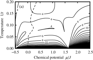
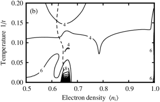
Figure 5: Contour diagrams showing the number of iterations required to reach a disordered phase sink in the $d=2$ isotropic $tJ$ model with $J/t=0.444$. Fig. 5(a) is plotted in terms of temperature vs. chemical potential, while Fig. 5(b) is in terms of temperature vs. electron density. Note the accumulation of contours towards the $\tau$ ranges of the chemical potential and density. The disorder line, along which the trajectories eventually cross over from the $\tau$ region to disorder, is shown as dashed.

Figure 6: Number of iterations required to reach a disordered phase sink in the $d=2$ isotropic $tJ$ model, plotted as a function of temperature for two different values of $\langle n_{i}\rangle$. The value $<n_{i}>=0.65$ is in the $\tau$ range.

In contrast to $d=3$ even with the weakest coupling between planes, in $d=2$ the $\tau$ phase sink is not a true sink fixed point of the recursion relations, but it is a ”quasisink” in the sense that renormalization-group flows come close, stay in its vicinity for many iterations, before crossing over along the disorder line to one of the disordered sinks. We thus find a zero-temperature $\tau$ critical point (which emerges from zero temperature with the slightest inclusion of interplanar coupling, leaving behind a true sink). The quasisink behavior is particularly true for trajectories initiating at low temperatures, where the quasisink that is reached is, numerically, essentially indistinguishable from a real one. Since regions of the phase diagram that are approximately basins of attraction of the quasisink are characterized by a sharp rise in the number of iterations required to eventually reach the disordered sinks, we can extract useful information by counting these iterations.

We choose a numerical cutoff for when the interaction constants in the rescaled Hamiltonian have come sufficiently close to their limiting values at any of the high-temperature disordered fixed points (the dilute disordered sink, the dense disordered sink, or the null fixed point in-between). We then count the number of iterations required to meet this cutoff condition for a given initial Hamiltonian. Fig. 5 shows the results as contour diagrams, plotted in terms of temperature vs. chemical potential and temperature vs. electron density. There are two clear regions in Fig. 5(a) where the number of iterations blows up at low temperatures. The region for $\mu/J$ approximately between -0.5 and 1.6 flows to the $\tau$ phase quasisink. When expressed in terms of electron density in Fig. 5(b), this region is centered around a narrow range of densities near $\langle n_{i}\rangle=0.65$, which is where the $\tau$ phase actually emerges for finite $t_{z}/t_{xy}$. The low-temperature region for $\mu/J\gtrsim 1.6$ flows to an antiferromagnetic quasisink, but does not appear in the electron density contour diagram because the entire region is mapped to $\langle n_{i}\rangle$ infinitesimally close to 1. This is similar to what we see in the anisotropic model for low $t_{z}/t_{xy}$, where the antiferromagnetic region is stable to only very small hole doping away from $\langle n_{i}\rangle=1$, but gradually spreads to larger doping values as the interplane coupling is increased. Fig. 6 shows the zero-temperature $\tau$ fixed point behavior in another way, by plotting the number of renormalization-group iterations as a function of temperature, for two different $\langle n_{i}\rangle$. For $\langle n_{i}\rangle=0.65$, in the $\tau$ phase range, the number of iterations diverges as temperature is decreased. In contrast, for $\langle n_{i}\rangle=0.75$, not in the $\tau$ phase range, the number is nearly constant at all temperatures. In summary, we see that the $d=2$ results are compatible with the small $t_{z}/t_{xy}$ limit of the anisotropic model. A weak interplane coupling stabilizes both the $\tau$ and antiferromagnetic phases, yielding finite transition temperatures.

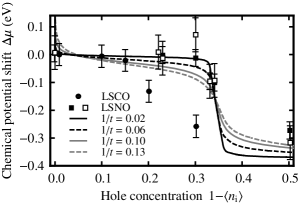
Figure 7: The calculated chemical potential shift $\Delta\mu$ is plotted as a function of hole concentration $1-\langle n_{i}\rangle$ for the isotropic $d=2$ $tJ$ model, at four different temperatures. For comparison with experimental results, the energy scale $\tilde{t}=0.1$ eV is chosen. With this scale, the temperatures $1/t=0.02$, $0.06$, $0.10$ and $0.13$ correspond to 23, 70, 116, and 151 K respectively. Experimental values for $\Delta\mu$ determined from x-ray photoemission spectra at $\sim 80$ K are shown for the cuprate La_2-xSr_xCuO₄ (LSCO, filled circles) AIno and the nickelate La_2-xSr_xNiO₄ (LSNO, filled squares) ASatake . For LSNO we also show another experimental estimate based on ultraviolet photoemission spectra (open squares), taken at 150 K, except for the datapoint at zero hole concentration, which was taken at 230 K ASatake .

We mentioned earlier that the lamellar structure of A and D phases which appears in the anisotropic $tJ$ phase diagram for hole dopings up to the $\tau$ phase might be an indicator of incommensurate ordering. One possible form this incommensurate ordering could take is the appearance of stripes, the segregation of the holes into D-like stripes where the hole kinetic energy is minimized, alternating with A-like stripes of antiferromagnetic order. Depending on the arrangement of such stripes with respect to the underlying lattice, the system could flow under repeated renormalization-group transformations either to the antiferromagnetic or dense disordered sink. Since the arrangement of the stripes will vary as we change the temperature or density in the system, this could lead to a lamellar structure of A and D phases in the resulting phase diagram. Though we cannot probe the existence of such stripes directly in our approach, an observable consequence of stripe formation would be the suppression of the chemical potential shift when additional holes are added to the system, since we effectively have a phase separation on a microscopic scale into hole-rich and hole-poor regions. Indeed, inquiries into stripe formation in experimental systems doped away from half-filling often look for this tell-tale pinning of the chemical potential. For example, in the cuprate superconductor La_2-xSr_xCuO₄ (LSCO), photoemission measurements of core levels have shown that the chemical potential shifts by a small amount ($<0.2$ eV/hole) in the underdoped region, $\delta\equiv 1-\langle n_{i}\rangle\lesssim 0.15$, compared to a large shift ($\sim 1.5$ eV/hole) in the overdoped region, $\delta\gtrsim 0.15$, an observation which has been interpreted as a possible signature of stripes AIno . In non-superconducting systems where the existence of stripes is clearly established, like the nickelate La_2-xSr_xNiO₄ (LSNO), we see a qualitatively similar behavior, with the chemical potential shifting significantly only for high-doping ($\delta\gtrsim 0.33$ for LSNO) ASatake . For the $tJ$ model, we take the chemical potential shift as $\Delta\mu=\tilde{\mu}-\tilde{\mu}_{0}$, where $\tilde{\mu}_{0}$ is the chemical potential below which $\langle n_{i}\rangle$ begins to the decrease noticeably from 1 in the low temperature limit. Fig. 7 shows our calculated $\Delta\mu$ vs. hole concentration for the $d=2$ $tJ$ model at four different temperatures. In order to compare with the experimental data for LSCO and LSNO, we choose an energy scale $\tilde{t}=0.1$ eV. For the low-doping region, where interplane coupling generates a lamellar structure of A and D phases, the slope of the $\Delta\mu$ curve remains small. On the other hand, for high-doping, in the range of densities corresponding to the $\tau$ phase, $\Delta\mu$ turns steeply downward. The similarities between this behavior and the experimental data supports the idea of stripe formation in the low-doping region.

- (1) E. Dagotto, Rev. Mod. Phys. 66, 763 (1994).
- (2) M. Imada, A. Fujimori, and Y. Tokura, Rev. Mod. Phys. 70, 1039 (1998).
- (3) S. Chakravarty, H.-Y. Kee, and K. Völker, Nature 428, 53 (2004).
- (4) L.P. Pryadko, S.A. Kivelson, and O. Zachar, Phys. Rev. Lett. 92, 067002 (2004).
- (5) T. Koretsune and M. Ogata, J. Phys. Soc. Japan 74, 1390 (2005).
- (6) W.O. Putikka and M.U. Luchini, cond-mat/0507430.
- (7) G. Su, Phys. Rev. B 72, 092510 (2005).
- (8) A. Falicov and A.N. Berker, Phys. Rev. B 51, 12458 (1995).
- (9) A. Falicov and A.N. Berker, Turk. J. Phys. 19, 127 (1995).
- (10) M. Hinczewski and A.N. Berker, Eur. Phys. J. B 48, 1 (2005).
- (11) M. Hinczewski and A.N. Berker, cond-mat/0503631; cond-mat/0607171.
- (12) A. Erbaş, A. Tuncer, B. Yücesoy, and A.N. Berker, Phys. Rev. E 72, 026129 (2005).
- (13) A.A. Migdal, Zh. Eksp. Teor. Fiz. 69, 1457 (1975) [Sov. Phys. JETP 42, 743 (1976)].
- (14) L.P. Kadanoff, Ann. Phys. (N.Y.) 100, 359 (1976).
- (15) A.N. Berker and S. Ostlund, J. Phys. C 12, 4961 (1979).
- (16) R.B. Griffiths and M. Kaufman, Phys. Rev. B 26, 5022 (1982).
- (17) M. Kaufman and R.B. Griffiths, Phys. Rev. B 30, 244 (1984).
- (18) M. Suzuki and H. Takano, Phys. Lett. A 69, 426 (1979).
- (19) H. Takano and M. Suzuki, J. Stat. Phys. 26, 635 (1981).
- (20) A.N. Berker, S. Ostlund, and F.A. Putnam, Phys. Rev. B 17, 3650 (1978).
- (21) R. Shankar and V.A. Singh, Phys. Rev. B 43, 5616 (1991).
- (22) C. Bernhard, J.L. Tallon, T. Blasius, A. Golnik, and C. Niedermayer, Phys. Rev. Lett. 86, 1614 (2001).
- (23) A.V. Puchkov, P. Fournier, T. Timusk, and N.N. Kolesnikov, Phys. Rev. Lett. 77, 1853 (1996).
- (24) L. Tan and J. Callaway, Phys. Rev. B 46, 5499 (1992).
- (25) D. Baeriswyl, C. Gros, and T.M. Rice, Phys. Rev. B 35, 8391 (1987).
- (26) J. Orenstein, G.A. Thomas, A.J. Millis, S.L. Cooper, D.H. Rapkine, T. Timusk, L.F. Schneemeyer, and J.V. Waszczak, Phys. Rev. B 42, 6342 (1990).
- (27) E. Dagotto and J. Riera, Phys. Rev. Lett. 70, 682 (1993).
- (28) E. Dagotto, J. Riera, Y.C. Chen, F. Alcaraz, and F. Ortolani, Phys. Rev. B 49, 3548 (1994).
- (29) M. Kohno, Phys. Rev. B 55, 1435 (1997).
- (30) H. Yokoyama and M. Ogata, J. Phys. Soc. Jap. 65, 3615 (1996).
- (31) S. Sorella, G.B. Martins, F. Becca, C. Gazza, L. Capriotti, A. Parola, and E. Dagotto, Phys. Rev. Lett. 88, 117002 (2002).
- (32) P.A. Lee, N. Nagaosa, and X.-G. Wen, Rev. Mod. Phys. 78, 17 (2006).
- (33) N.D. Mermin and H. Wagner, Phys. Rev. Lett. 17, 1133 (1966).
- (34) A. Ino, T. Mizokawa, A. Fujimori, K. Tamasaku, H. Eisaki, S. Uchida, T. Kimura, T. Sasagawa, and K. Kishio, Phys. Rev. Lett. 79, 2101 (1997).
- (35) M. Satake, K. Kobayashi, T. Mizokawa, A. Fujimori, T. Tanabe, T. Katsufuji, and Y. Tokura, Phys. Rev. B 61, 15515 (2000).