Supersonic rupture of rubber

Abstract

The rupture of rubber differs from conventional fracture. It is supersonic, and the speed is determined by strain levels ahead of the tip rather than total strain energy as for ordinary cracks. Dissipation plays a very important role in allowing the propagation of ruptures, and the back edges of ruptures must toughen as they contract, or the rupture is unstable. This article presents several levels of theoretical description of this phenomenon: first, a numerical procedure capable of incorporating large extensions, dynamics, and bond rupture; second, a simple continuum model that can be solved analytically, and which reproduces several features of elementary shock physics; and third, an analytically solvable discrete model that accurately reproduces numerical and experimental results, and explains the scaling laws that underly this new failure mode. Predictions for rupture speed compare well with experiment.

March 8, 2024

1 Introduction

The theory of fracture was originally developed to explain the failure of brittle materials, where cracks have a number of common features (Irwin, 1957; Kanninen and Popelar, 1985; Thomson, 1986). A stress singularity builds up in the vicinity of the tip. Stresses diverge as $1/\sqrt{r}$, where $r$ is the distance to the tip. The displacement of material near the tip behaves as $\sqrt{r},$ which means that the tip viewed closely has the shape of a sideways parabola. Energy flows in towards the crack from far away and concentrates itself at the tip in just the amount needed to snap bonds and feed other dissipative processes. Partly for this reason, cracks in tension cannot travel faster than the Rayleigh wave speed, which is the speed at which sound travels across a free surface(Broberg, 1999; Freund, 1990).

Experimental evidence has accumulated showing that the rapid rupture of rubber sheets, such as when one pops a balloon, is different. If one cuts a horizontal slit in a rubber sheet and stretches it up, the opening profile is a sideways parabola, as expected for static cracks. Once the rupture begins to run, however, the characteristic $\sqrt{r}$ opening displacement disappears, and is replaced by a wedge-like shape (Deegan et al., 2002). Furthermore, the rupture speed exceeds the shear wave speed in advance of the tip (Petersan et al., 2004). However the extensions in rubber when it ruptures are very large. The ordinary theory of fracture begins with the assumption that strains are very small, typically on the order of a fraction of a percent far ahead of the crack. In rubber, rupture initiates when strains are on the order of several hundred percent. Therefore it is not clear how much of fracture mechanics ought to apply to rubber, and whether the violations of rules about rupture speed are simply the natural result for a material that breaks for very large extensions, or whether the mode of failure is something new.

In this article I will explain the case first outlined in Marder (2005) that the rupture of rubber is different from conventional fracture. It is a tensile failure. The ruptures always travel faster than the shear wave speed. The opening is a wedge that obeys a simple relation that applies to Mach cones. Stress is singular near the tip, but strain is not, and material in front of the tip must be brought rather near the point of failure for ruptures to propagate.

Buehler, Gao, and Abraham (2003) have proposed that hyperelasticity plays a critical role in dynamic fracture, and that in particular an increase of sound speed near a crack tip can allow cracks to travel faster than the distant shear wave speed. In the analysis of this paper, there is an increase of elastic modulus near the tip of the rupture, but it is not in the form that Buehler, Gao, and Abraham proposed. The theory here relies upon an increase in the modulus of rubber with frequency, rather than upon the increase in modulus of rubber with extension. The low-frequency modulus of real rubber certainly increases as rubber stretches towards the breaking point (Treloar, 1975, p. 2). However, I found in numerical investigations that the behavior of ruptures does not change appreciably whether such stiffening prior to breakage is included or not. In the computations of this paper, Lagrangean sound speeds are either independent of extension (Sections 5 and 6), or else increase as the rubber contracts (Section 4.3). In view of the fairly detailed comparison of theory, numerical work, and experiment obtained in this work, the conclusion is that static hyperelasticity is not relevant to the supersonic rupture of rubber.

The theory comes in several forms. I begin with a numerical model of rubber that is fairly realistic and includes most of the physical features of rubber indicated by experiment. There are only three parameters in this model not determined directly from experiment, and of those there is only one to which the fracture dynamics are particularly sensitive. Next, I note that after stripping some of the realistic complexity out of the numerical model, the dynamics of ruptures scarcely change. The resulting theory is so simple that it can be solved analytically. The analytical solution takes two forms. The first is a continuum model with a simple failure criterion that leads to compact closed-form expressions for rupture speed and opening angle. The expressions for rupture velocity agree with laboratory data within experimental error, although they disagree with rupture speeds from numerical modeling by around 10%. Finally, the discrete rupture theory has a complete analytical solution. This solution enables one to see the relation between the conventional theory of fracture and supersonic ruptures, and is particular how these two types of solution scale in the macroscopic limit.

The structure of the paper is as follows: Section 2 presents some elementary physical ideas to describe rubber rupture. Section 3 lays out the continuum energy functional for rubber on which much of the subsequent discussion will be based. Section 4 develops a computational method that makes it possible to obtain numerical solutions that mimic the main features of experimental ruptures. Section 5 extracts from the numerical model a simple continuum theory and presents its solution. Section 6 proceeds further to obtain an exact analytical solution of the full numerical model, after some simplifications. Section 7 compares theoretical predictions with the experimental results. There are also five appendices, which discuss (A) how to obtain an effective two–dimensional theory from the original three–dimensional theory, (B) the computation of sound speeds from the two–dimensional continuum theory, (C) the computation of forces for the numerical model, (D) a lattice instability found in some of the numerical models, and (E) the solution of the discrete model by Wiener-Hopf techniques.

2 Elementary considerations

Much of this paper will be concerned with the speed of ruptures in rubber. Therefore it is necessary to begin by describing precisely how speed will be defined. Suppose that a sound wave or a rupture travels through a highly stretched rubber sheet. One can choose either to describe its speed in the laboratory (Eulerian sound speed) or back in a coordinate system tied to the original location of mass points (Lagrangean sound speed). To be more explicit, consider a sheet of rubber lying relaxed in some initial material reference configuration. Describe the sheet in this configuration with the variable $\vec{r,}$ which serves as a label for mass points. Once the rubber is stretched and begins to move, the new locations of mass points will be given by the variable $\vec{u.}$ Now consider some deformation or bump moving through the rubber at constant speed. The maximum amplitude of the bump is located at some point $\vec{u}(t)$ which changes in time, and the speed at which it moves is the laboratory velocity. However, there is another velocity, which from a theoretical point of view is much more natural to employ, and which helps assemble the experimental results into a compact scaling form. Whenever the bump is located at $\vec{u,}$ one can identify the original location $\vec{r}$ of the mass point now at the center of the bump, and $\vec{r(t)}$ also evolves in time. The speed at which $\vec{r(t)}$ travels is the Lagrangean speed, and unless otherwise specified, sound and rupture speeds will always be measured in this Lagrangean reference system. For example, if one considers a bump of small amplitude moving along $x$ in rubber that has been stretched by a factor of $\lambda_{x}$ above its original length, then the speed of the bump in the laboratory frame exceeds that in the reference frame by a factor of $\lambda_{x}$ .

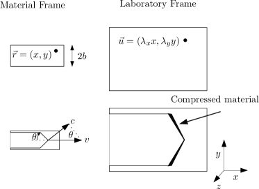
Figure 1: Illustration of material and laboratory frames used to describe rupture of rubber. The top left panel shows a rubber sheet before it has been stretched, and the top right shows it stretched by amounts $\lambda_{x}$ and $\lambda_{y}$ in the $x$ and $y$ directions. The lower right panel shows a traveling rupture as seen in the laboratory, while the lower left shows the same rupture back in the material frame. If the normal velocity of the rupture is $c,$ then the forward velocity of the rupture must be $v\sin\theta.$ The shock lines shown in the lower left panel correspond to the leading edge of compressed material in the lower right panel.

Now consider a thin sheet of rubber that is stretched by factors of $\lambda_{x}$ and $\lambda_{y}$ in the $x$ and $y$ directions respectively, as shown in Figure 1. Stick a pin into the sheet on the left hand side so that a rupture runs to the right along the $x$ direction. One sees in experiment (Petersan et al., 2004; Deegan et al., 2002) that the rupture consists in two straight fronts that meet at a point, forming a wedge. Suppose that the two straight fronts are shock fronts, traveling at the Lagrangean wave speed $c.$ As is customary for the elementary theory of shocks (Serway and Beichner, 2000, p. 534), the speed $v$ of the tip of the rupture must obey

$$\frac{c}{v}=\sin\theta,$$ (1)

where $\theta$ is the opening angle of the rupture, as shown in Figure 1. The slope of the upper face of the shock line is $-\tan\theta,$ which is

$$\textrm{material frame slope }=-\frac{1}{\sqrt{v^{2}/c^{2}-1}}.$$ (2)

In the laboratory, where distances are stretched by factors of $\lambda_{x}$ and $\lambda_{y}$, the slope will intead be

$$\textrm{laboratory slope = }-\frac{\lambda_{y}}{\lambda_{x}\sqrt{v^{2}/c^{2}-1}},$$ (3)

since if one draws a line of slope $\alpha$ on a sheet of rubber and stretches it along $x$ by a factor of $\lambda_{x}$, the slope decreases by a factor of $\lambda_{x}.$

Eq. (3) will re-emerge from detailed calculations as Eq. (69). The main physical quantity left undetermined is the rupture velocity $v$. A decent approximate relation, obtained as Eq. (79) that closes the theory is

$$\lambda_{f}^{2}=\frac{1}{4}\lambda_{x}^{2}+\frac{3}{4}\lambda_{y}^{2}/(1-c^{2}/v^{2}),$$

where $\lambda_{f}$ is an extension at which polymers in rubber snap. Far ahead of the rupture, the bonds that will eventually be brought to the snapping point are already stretched an amount $\sqrt{\frac{1}{4}\lambda_{x}^{2}+\frac{3}{4}\lambda_{y}^{2}}$ over their original length. In simple physical terms, then, the assertion is that just in front of the tip of the rupture, material stretches by an additional factor of $1/(1-c^{2}/v^{2})$ in the vertical direction. However, I have not found an elementary argument to produce this relation.

3 Continuum Energy Functional

3.1 Coordinate system and definition of energy functional

Strains in rubber are several hundred percent at rupture and one must use nonlinear elastic theory to describe the situation (Atkin and Fox, 1980; Ogden, 1984). I state just enough of the theory to establish notation. Adopt a description of a highly deformed rubber sheet with

$$\vec{r}=(r_{x},r_{y})=(x,y)\mapsto\vec{u}=(u^{x},u^{y}).$$ (4)

The original location of all mass points is given by $\vec{r}$ and the location of points after the rubber is moved and stretched is given by $\vec{u}.$ Note that $\vec{u}$ is measured from the origin, not from the original location of the mass point $\vec{r}.$ Define the Lagrangean strain tensor

$$E_{\alpha\beta}\equiv\mbox{$\frac{1}{2}$}\left[\sum_{\gamma}\frac{\partial u^{\gamma}}{\partial r_{\alpha}}\frac{\partial u^{\gamma}}{\partial r_{\beta}}-\delta_{\alpha\beta}\right].$$ (5)

From this strain tensor one can define three rotationally invariant quantities. These are

$$I_{1}^{3D} = {\rm Tr\,}E$$ (6a)

$$I_{2}^{3D} = \sum_{\alpha<\beta}\left[E_{\alpha\alpha}E_{\beta\beta}-E_{\alpha\beta}^{2}\right]$$ (6b)

$$I_{3}^{3D} = {\rm det}\,E,$$ (6c)

Rubber is highly incompressible (Treloar, 1975, p. 61). Accordingly, for a thin sheet of rubber, one can express the thickness at every point in terms of the strains in the $x-y$ plane, and project the theory into two dimensions, as discussed in Appendix A. In two dimensions one has only the two invariants,

$$I_{1}={\rm Tr}\,E;\quad I_{2}=E_{xx}E_{yy}-E_{xy}^{2},$$ (7)

and using the incompressibility of rubber to solve for $E_{zz}$ one finds

$$E_{zz}=\mbox{$\frac{1}{2}$}\left(\frac{1}{4I_{2}+2I_{1}+1}-1\right),$$ (8)

in terms of which the first two of the three–dimensional strain invariants take the form

$$I_{1}^{3D} = I_{1}+E_{zz}$$

$$I_{2}^{3D} = I_{2}+E_{zz}I_{1}$$ (9)

The energy density of a thin sheet of rubber is then taken to be given by some function $e$ of $I_{1}$ and $I_{2},$ and the total energy $U$ is

$$U=\rho\int d\vec{r^{\prime}}\>e\left(I_{1}(\vec{r^{\prime}}),I_{2}(\vec{r^{\prime}})\right).$$ (10)

The integral is performed in the material frame, and the mass density $\rho$ is also measured in the material frame.

An energy-conserving equation of motion for this theory is

$$0=\frac{\delta}{\delta u^{\gamma}(\vec{r)}}\left[\int d\vec{r}^{\prime}\ {\textstyle\frac{1}{2}}\rho\left|\dot{\vec{u}}\right|^{2}-\rho e\right],$$ (11)

where $\rho$ is the mass per area, again measured in the material frame. Performing the functional derivatives, one has

$$\rho\ddot{u}^{\gamma}=-\frac{\delta U}{\delta u^{\gamma}(\vec{r})}.$$ (12)

Appendix A demonstrates that this equation of motion for a two-dimensional sheet obtained by calculating $E_{zz}$ through Eq. (8) is the same one obtains from the Piola-Kirkhoff stress tensor after imposing incompressibility and requiring that the Cauchy stress $T_{zz}$vanish.

3.2 Sound Speeds

The experiments by Petersan et al. (2004) that stimulated this study obtained detailed information about the speed of sound in rubber under a range of loading conditions. For a while, we found the results puzzling, but eventually realized that they could all easily be explained by the Mooney-Rivlin theory. Appendix B contains a sketch of how to obtain sound speeds from the equation of motion (12). Here I record only the final results, all of which are standard(Eringen and Suhubi, 1974, v. 1, pp. 120, 263). Suppose that a rubber sheet is strained uniformly with displacement field

$$\vec{u}=(\lambda_{x}x+s_{xy}y,\lambda_{y}y+s_{yx}x).$$ (13)

Look for the speed of sound along the $x$ and $y$ axes of a sample that is extended by the two factors $\lambda_{x}$ and $\lambda_{y}$; $s_{xy}$ and $s_{yx}$ are included in Eq. (13) only because one must be able to perform calculations involving small virtual shears around this base state. Then there is a longitudinal sound wave along the $x$ axis whose speed with $s_{xy}=s_{yx}=0$ is

$$c_{xl}^{2}=\frac{\partial^{2}e}{\partial\lambda_{x}^{2}}.$$ (14a)

Similarly, the speed of longitudinal waves in the $y$ direction is

$$c_{yl}^{2}=\frac{\partial^{2}e}{\partial\lambda_{y}^{2}}.$$ (14b)

There is also a shear wave that travels along $x$ and is polarized along $y$ with speed

$$c_{xs}^{2}=\frac{\partial^{2}e}{\partial s_{yx}^{2}}.$$ (14c)

Similarly a wave traveling along $y$ and polarized along $x$ has speed

$$c_{ys}^{2}=\frac{\partial^{2}e}{\partial s_{xy}^{2}}.$$ (14d)

Alternatively, one can express sounds speeds in terms of derivatives with respect to strain tensor components. One has for the longitudinal wave speed along $x$,

$$c_{lx}^{2}=\frac{\partial e}{\partial E_{xx}}+\lambda_{x}^{2}\frac{\partial^{2}e}{\partial E_{xx}^{2}}$$ (15a)

while for the shear wave speed (setting $E_{yx}=E_{xy}$ before taking the derivatives)

$$c_{sx}^{2}=\frac{\partial e}{\partial E_{xx}}+\frac{\lambda_{y}^{2}}{4}\frac{\partial^{2}e}{\partial E_{xy}^{2}}.$$ (15b)

All of these speeds are Lagrangean speeds, as described in Section 3.1.

Sound speeds provide a convenient way to assemble experimental data about the constitutive behavior of rubber. In some cases, sound speeds are measured directly through time of flight, while in other cases they are measured through small extensions of the sample around a base state as suggested by Eqs. (3.2). The results of Petersan et al. (2004) are quite simple. Over a range of biaxial states where $\lambda_{x}\in[2,3.5]$ and $\lambda_{y}\in[2,3.5]$ the Lagrangean wave speeds appear to be constant, with the longitudinal wave speed around 20% greater than the shear wave speed. From Eqs. (15b) one finds that this is not possible. The only way for the longitudinal and shear wave speeds both to be constant is to adopt $e(I_{1},I_{2})\propto I_{1},$ and in this case the longitudinal and shear wave speeds must be equal.

This apparent difficulty is resolved by examining a bit more carefully the free energy functional due to Mooney and Rivlin(Treloar, 1975; Mooney, 1940; Rivlin, 1948a, b). The Mooney–Rivlin theory says that the free energy density of rubber is

$$U/\rho\equiv e=A(I_{1}^{3D}+BI_{2}^{3D}),$$ (16)

where $U$ has units of energy per volume, $\rho$ is mass density, $A$ is a constant with units of velocity squared, and $B$ is dimensionless. Using Eq. (9) one obtains an effective two–dimensional Mooney–Rivlin theory

$$e(I_{1},I_{2})=A\left(I_{1}+BI_{2}+E_{zz}(1+BI_{2})\right)$$ (17)

For extensions $\lambda_{x}$ and $\lambda_{y}$ on the order of 2 or greater, $E_{zz}+1/2$ is of order $1/(\lambda_{x}^{2}\lambda_{y}^{2})$ and is at least 64 times smaller than $E_{xx}$ or $E_{yy}$. Therefore, for the purpose of examining the experiments, it is sufficient to use

$$e(I_{1},I_{2})=A(I_{1}+BI_{2})=A\left[(E_{xx}+E_{yy})+B\left(E_{xx}E_{yy}-E_{xy}^{2}\right)\right]$$ (18)

Employing Eqs. (15b) and (18)one finds for longitudinal and shear wave speeds

$$c_{xl}^{2} = A\left[1+\frac{B}{2}(\lambda_{y}^{2}-1)\right];\ \$$ (19a)

$$c_{yl}^{2} = A\left[1+\frac{B}{2}(\lambda_{x}^{2}-1)\right];$$ (19b)

$$c_{xs}^{2} = c_{ys}^{2}=A\left[1-\frac{B}{2}\right].$$ (19c)

Thus for a Mooney–Rivlin material the shear wave speed is constant, and the longitudinal speed along $x$ is independent of $\lambda_{x}$ but depends quadratically on $\lambda_{y}$. Turning to the experimental data, one finds that they are consistent with these observations as shown in Fig. 2, and that one can fix the constants $A$ and $B$.

(A)

(B)

Figure 2: (A) Sound speed data for various values of $\lambda_{x},$ and $\lambda_{y}=3.2.$ Experimental longitudinal ($c_{xl}=\square)$ and shear ($c_{xs}=\blacksquare$) speeds are shown in the material frame. They are roughly constant, and can be fit by (19a) (—) and (19c) ($\dots\dots$), using $A=501\ \mbox{(m/s})^{2},$ $\ B=0.106$. The shear wave speed comes out to 21.8 m/s and the longitudinal wave speed for $\lambda_{y}=3.2$ is 27.3. (B) Using the constants $A$ and $B$ obtained from the data in (A), calculate longitudinal wave speeds in the $y$ direction $c_{yl}$. According to Eq. 3.2, this is the only speed that varies as a function of $\lambda_{x}$. The agreement with the data is satisfactory.

For studying the rupture of rubber, the energy density in Eq. (17) is both too simple and too complicated. It is too simple because it does not account for the fact that when rubber is stretched enough, the polymers pull apart and the force between adjacent regions drops irreversibly to zero. It is too complicated because the terms involving $I_{2}$ and $E_{zz}$ produce nonlinear equations of motion that are impossible to solve analytically. Therefore, to analyze the problem, I will pursue two different routes. First, I will discuss numerical routines that supplement Eq. (17) with information about rupture, toughening, and dissipation, and produce supersonic solutions. Second, I will isolate from Eq. (17) terms that are sufficient to produce good agreement with numerics and experiment, while simplifying matters enough to permit analytical solution.

4 Numerical methodology

For the problem of fracture, there are great advantages to thinking in terms of molecular dynamics. From a continuum viewpoint, it is difficult to understand how to construct a physically sensible theory where material gives way. From an atomic viewpoint it is easy; when two atoms are separated by more than a certain distance, they stop applying force to one another. Therefore, I have found a simple set of microscopic interactions that produces the Mooney–Rivlin theory of Eq. (17) in the continuum limit. The interacting mass-points that appear in the theory should not be thought of as atoms. To describe rubber, they should be thought of as nodes in a cross-linked polymer network, with a characteristic spacing of around a micron. There are some possible objections to this approach. Rubber is much more complex than a triangular lattice, mass is distributed rather than being concentrated at nodes, and one might worry about the fact that the two-dimensional array of nodes has been engineered to reproduce dynamics that derive from projections into two dimensions of three-dimensional equations of motion. There is no complete answer to these objections; the best response is to show that the resulting theory provides detailed correspondence with experiment, and allows much analytical and numerical progress.

Similar numerical techniques have been used before; for example by Seung and Nelson (1988). The techniques of that paper must be extended to include bond snapping and dissipation, which I carry out here. The philosophy is also similar to the Virtual Internal Bond method (Gao and Klein, 1998; Klein and Gao, 1998) and the Peridynamic Model (Silling and Bobaru, 2005; Silling, 2000), which also focus on a collection of discrete interacting mass points considerably larger than atoms in order to obtain rules for fracture. However, all details of the implementation of this idea are different; the formulation presented here has the advantage of leading in one case to a discrete model of nonlinear materials with a complete analytical solution.

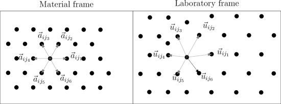
Figure 3: Diagram showing triangular lattice of lattice spacing $a$ and nearest-neighbor vectors $\vec{a_{ij}}$ used in this section. The original locations of particles at rest are given by $\vec{a,}$ while their location in the laboratory after deformation is given by $\vec{u}.$

4.1 Low-order polynomial terms for microscopic theory

Consider the triangular lattice depicted in Fig. 3. The figure shows the original locations of all particles prior to any distortion, denoted by $\vec{a}_{i},$ and the lattice spacing is $a.$ After distortion, the position of particles in the laboratory is given by $\vec{u_{i}}$The goal is to construct a theory for the energy required to displace particles on this lattice that involves $I_{1}$ and $I_{2}$, and employs quadratic and quartic functions of displacements $u.$ It is possible to construct such a theory by considering simple combinations of rotationally invariant operations on nearest-neighbor vectors. Let $\vec{u_{ij}}\equiv\vec{u_{j}}-\vec{u}_{i},$ let $n(i)$ refer to the nearest neighbors of $i$, and define

$$F_{i}=\frac{1}{6}\sum_{j\in n(i)}\begin{cases}\left(\vec{u}_{ij}\cdot\vec{u}_{ij}-a^{2}\right)&\textrm{if }u_{ij}<\lambda_{f}\\ \lambda_{f}^{2}-a^{2}&\textrm{else}\end{cases}$$ (20a)

$$G_{i}=\frac{1}{9}\sum_{j\in n(i)}\begin{cases}\left(\vec{u}_{ij}\cdot\vec{u}_{ij}-a^{2}\right)^{2}&\textrm{if }u_{ij}<\lambda_{f}\\ \left(\lambda_{f}^{2}-a^{2}\right)^{2}&\textrm{else}\end{cases}$$ (20b)

$$H_{i}=\frac{1}{27}\sum_{j\neq k\in n(i)}h(u_{ij})h(u_{ik})\left(\vec{u}_{ij}\cdot\vec{u}_{ik}+2a^{2}\right)^{2},$$ (20c)

$$\mbox{and}\quad h(u)=1/(1+e^{(u-\lambda_{f})/u_{s}}).$$ (20d)

The sums are carried out over the 6 nearest neighbors of point $i$ shown in Fig. 3. The terms are constructed so as to become constant and therefore describe breaking bonds when $u_{ij}$ increases to more than $\lambda_{f}$. The final term requires a cutoff function $h$ since this is the only way to ensure both that $H_{i}$ be continuous, and that it settle down to a constant value when $u_{ij}$ or $u_{ik}$ are large; the constant $u_{s}$ describes the scale over which $h$ vanishes. Terms of this form are standard in molecular dynamics (e.g. Stillinger and Weber (1985)). To form a correspondence with continuum theory, suppose that no bonds are stretched past the breaking point ($u_{ij}<\lambda_{f})$, and approximate the position of neighbors of point $i$ by

$$u_{ij}^{\alpha}\approx\sum_{\beta}a_{ij}^{\beta}\frac{\partial}{\partial x^{\beta}}u^{\alpha}(\vec{r})$$ (21)

Insert Eq. (21) into Eqs. (20a) to obtain (using Eq. (5))

$$F_{i} \approx \frac{1}{6}\sum_{j\in n(i)}\left(\sum_{\alpha\beta\gamma}a_{ij}^{\beta}\frac{\partial u^{\alpha}}{\partial x_{\beta}}\frac{\partial u^{\alpha}}{\partial x_{\gamma}}a_{ij}^{\gamma}-a^{2}\right)$$

$$= \frac{1}{6}\sum_{j\in(i)}\left(\sum_{\beta\gamma}a_{ij}^{\beta}\left[2E_{\beta\gamma}+\delta_{\beta\gamma}\right]a_{ij}^{\gamma}-a^{2}\right)$$

$$= (E_{xx}+E_{yy})a^{2}=I_{1}a^{2},$$ (23)

$$G_{i} \approx \frac{1}{9}\sum_{j\in n(i)}\left(\sum_{\alpha\beta\gamma}a_{ij}^{\beta}\frac{\partial u^{\alpha}}{\partial x_{\beta}}\frac{\partial u^{\alpha}}{\partial x_{\gamma}}a_{ij}^{\gamma}-a^{2}\right)^{2}$$ (24)

$$=\frac{1}{9} \sum_{j\in n(i)}\left(\sum_{\alpha\beta\gamma}a_{ij}^{\beta}\left[2E_{\beta\gamma}+\delta_{\beta\gamma}\right]a_{ij}^{\gamma}-a^{2}\right)^{2}$$

$$= \left[(E_{xx}+E_{yy})^{2}+\frac{4}{3}\left(E_{xy}^{2}-E_{xx}E_{yy}\right)\right]a^{4}$$

$$= \left[I_{1}^{2}-\frac{4}{3}I_{2}\right]a^{4}$$

$$H_{i} \approx {\textstyle\frac{1}{27}}\sum_{j\neq k\in n(i)}\left(\sum_{\alpha\beta\gamma}a_{ij}^{\beta}\frac{\partial u^{\alpha}}{\partial x_{\beta}}\frac{\partial u^{\alpha}}{\partial x_{\gamma}}a_{ik}^{\gamma}+2a^{2}\right)^{2}$$

$$=\frac{1}{27} \sum_{j\neq k\in n(i)}\left(\sum_{\alpha\beta\gamma}a_{ij}^{\beta}\left[2E_{\beta\gamma}+\delta_{\beta\gamma}\right]a_{ik}^{\gamma}+2a^{2}\right)^{2}$$

$$= \left[(E_{xx}+E_{yy})^{2}+\frac{20}{9}\left(E_{xy}^{2}-E_{xx}E_{yy}\right)+4\right]a^{4}$$

$$= \left[I_{1}^{2}-\frac{20}{9}I_{2}+4\right]a^{4}.$$ (26)

Comparing Eqs. (24), (4.1), and (4.1) with Eq. (7) gives

$$I_{1}^{i}=\frac{F_{i}}{a^{2}}$$ (27)

$$I_{2}^{i}=\frac{3}{4}\frac{1}{a^{4}}\left(F_{i}^{2}-G_{i}\right),$$ (28)

or alternatively,

$$I_{2}^{i}=\frac{9}{8}\frac{1}{a^{4}}\left(G_{i}-H_{i}+4\right).$$ (29)

Numerically, Eq. (28) is much less costly to compute than Eq. (29). However, Eq. (28) has the unfortunate property that under biaxial strain, spatially uniform states are unstable when this representation of $I_{2}$ is employed. Particles bunch up in a non–uniform way within each unit cell, forming stripes on a microscopic scale, as shown in Appendix C. It could be that this behavior is related to the physical phenomenon of strain crystallization (Treloar, 1975, p. 20). However, as strain crystallization does not occur experimentally in the range of extensions where ruptures are observed, I have largely employed Eq. (29) in preference to Eq. (28).

4.2 Specification of numerical energy functional

To form a numerical representation of Eq. (10), take

$$U=m\sum_{i}e(I_{1}^{i},I_{2}^{i}),$$ (30)

where $m$ is the mass in a unit cell. Then if $\Omega$ is the volume of a unit cell,

$$U\approx\frac{m}{\Omega}\int d\vec{r}\ e\big{(}I_{1}(\vec{r}),I_{2}(\vec{r})\big{)},$$ (31)

so since $m/\Omega=\rho,$ $e$ in Eq. (30)corresponds to $e$ in the continuum theory, and has units of velocity squared. In particular, for the Mooney–Rivlin theory, one has

$$e(I_{1}^{i},I_{2}^{i})=A(I_{1}^{i}+BI_{2}^{i}+E_{zz}^{i}(1+BI_{2}^{i}),$$ (32)

where $I_{1}^{i}$ is given by Eq. (27), $I_{2}^{i}$ is given either by Eqs. (28) or (29) , and $E_{zz}^{i}$ is given by(8), with $I_{1}^{i}$ and $I_{2}^{i}$ substituted for $I_{1}$ and $I_{2}$ .

4.3 Equation of Motion

Given the energy functional (30) one can obtain the force on every particle and therefore an equation of motion. In addition to the conservative force resulting from derivatives of the energy, add Kelvin dissipation, so that the complete equation of motion reads

$$m\ddot{u}_{i}^{\alpha}=-\partial U/\partial u_{i}^{\alpha}+\sum_{j\in n(i)}\frac{2mA\beta}{3a^{2}}\dot{u}_{ij}^{\alpha}\theta(\lambda_{f}-u_{ij}).$$ (33)

The final term in Eq. (33) represents the Kelvin dissipation, and is the simplest dissipative term permitted by symmetry. The motion of each mass point dissipates some energy in proportion to its velocity relative to each neighbor. This dissipation vanishes when the bond between two neighbors breaks.

The computation of $\partial U/\partial u_{i}^{\alpha}$ is not particularly difficult as force computations go. A formalism that makes it easy to exploit symmetry to reduce the amount of computation is briefly described in Appendix C.

One final rule is employed in the numerical runs, although it is not indicated explicitly in Eq. (33). Whenever some bond $u_{ij}$ drops to a length less than $1.5a$, the failure extension $\lambda_{f}$ for the remaining bonds attached to nodes $i$ and $j$ increases. Without some rule of this type, the back faces of the crack disintegrate. The reason for this rule will be explained in Section 5.3.

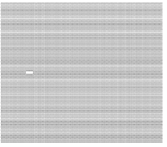
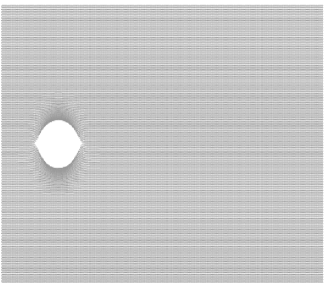
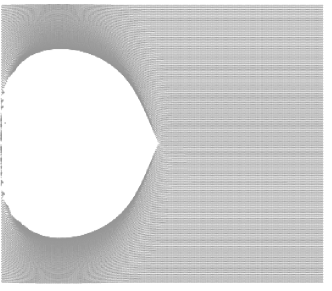
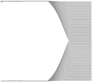
Figure 4: Four panels showing initiation of rupture in numerical sheet of rubber. The numerical system contains around 70,000 particles, and solves Eq. (33), using Eqs. (30) and (32) with $A=501$m${}^{2}/$s${}^{2},$ $B=.106,$ $\lambda_{f}=5.5,$ and $\beta=3.$ The first panel shows the initial pop, the second shows the system 12.5 time units later, the third after 25 time units, and the final panel after 250 time units, where the time unit is $a/\sqrt{A}$ .

Figure 4 shows characteristic panels from a numerical solution of Eq. (33). First, one prepares a uniformly strained sheet, in this case with extensions $\lambda_{x}=2.2,$ $\lambda_{y}=3.2.$ Next, two rows of particles are selected near the left hand side of the sample: the rows are five particles wide, and they sit right on top of one another. The upper particles are given a large upward velocity, and the lower particles are given a large downward velocity. This initial condition has the effect of popping a hole in the strip. As shown in the subsequent panels of Figure 4, the hole initially develops in a circular fashion, but as it senses the upper and lower boundaries, it begins to run sideways, and eventually turns into a shock-like rupture front that travels in steady state indefinitely to the right.

Figure 5 shows a comparison of experimental rupture velocities once steady state has been reached with results from numerical simulations. The agreement is satisfactory. However, the figure also contains the results of a different set of simulations. In these, Eq. (33) is solved not with the Mooney-Rivlin energy function in Eq. (32), but with a much simplified Neo–Hookean energy functional

$$e_{NH}(I_{1}^{i},I_{2}^{i})=c^{2}I_{1}^{i}.$$ (34)

The velocity of ruptures described by this very simple theory is indistinguishable from the velocity of ruptures described by the more elaborate Mooney-Rivlin theory. This observation opens the way to accurate analytical descriptions of the rupture of rubber, both at the continuum and discrete levels.

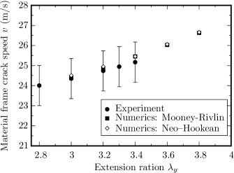
Figure 5: Comparison of experimental crack speeds and speeds in simulation. Simulations and experiments are conducted with $\lambda_{x}=2.2,$ and a range of vertical extensions $\lambda_{y}$ .The parameters describing the properties of the continuum nonlinear elastic theory are $A=501\ \mbox{(m/s})^{2},$ $\ B=0.106$, as in Figure 2. Bonds in the simulation fail when extended an amount $\lambda_{f}=5.5$ above their original length. The magnitude of Kelvin dissipation is $\beta=3$. In addition, the figure displays results from a substantially simplified numerical model where $B=0,$ and where $E_{zz}$ is set to zero as well. Stripping most of the complexity from the numerics has little effect on the results.

5 Continuum Neo–Hookean theory

5.1 Cracks in the Neo–Hookean theory

The continuum Neo–Hookean energy is

$$e_{NH}=AI_{1}=\frac{A}{2}\left[\left(\frac{\partial u^{x}}{\partial x}\right)^{2}+\left(\frac{\partial u^{x}}{\partial y}\right)^{2}+\left(\frac{\partial u^{y}}{\partial x}\right)^{2}+\left(\frac{\partial u^{y}}{\partial y}\right)^{2}\right].$$ (35)

This energy functional was first employed for the study of rubber by Mooney (1940), and was employed for the study of fractures by Klingbeil and Shield (1966). It has a number of interesting properties. Because it is quadratic in displacements, it leads to a linear equation of motion for $\vec{u,}$ which is easy to approach analytically. Nevertheless, it describes very large displacements of rubber, and in that sense is still a nonlinear theory. According to Eq. (3.2), there is only one sound speed for this theory,

$$c^{2}=A.$$ (36)

The equation of motion of the Neo–Hookean theory follows from Eqs (4.1), (30), and (33), and is

$$m\ddot{u}_{i}^{\alpha}=\sum_{j\in n(i)}\frac{2mc^{2}}{3a^{2}}\left(u_{ij}^{\alpha}+\beta\dot{u}_{ij}^{\alpha}\right)\theta(\lambda_{f}-u_{ij}).$$ (37)

In the continuum limit, overlooking bond rupture, one has

$$m\ddot{u_{i}}^{\alpha} = \frac{2mc^{2}}{3a^{2}}\sum_{j\in n(i)}(u_{j}^{\alpha}-u_{i}^{\alpha})+\beta(\dot{u}_{j}^{\alpha}-\dot{u}_{i}^{\alpha})$$

$$= \frac{mc^{2}}{3a^{2}}\sum_{\vec{a}\alpha\gamma}\frac{\partial^{2}(u^{\alpha}+\beta\dot{u}^{\alpha})}{\partial r_{\alpha}\partial r_{\gamma}}a_{ij}^{\alpha}a_{ij}^{\gamma}$$

$$= mc^{2}\nabla^{2}(u^{\alpha}+\beta\dot{u}^{\alpha})$$

For the study of fracture, there are some additional simplifications that arise in simple geometries. Consider a semi-infinite crack moving along the center line of an infinitely long strip as illustrated in Figure 1. The bottom of the strip is held at height $-b\lambda_{y}$, while the top of the strip is raised rigidly to height $\lambda_{y}b,$ where $2b$ is the original height of the strip. Suppose that the rubber is initially stretched by a factor $\lambda_{x}$ everywhere in the horizontal direction. Dropping for the moment Kelvin dissipation, the equation of motion is

$$\ddot{u}^{x}=c^{2}\nabla^{2}u^{x}$$ (39a)

$$\ddot{u}^{y}=c^{2}\nabla^{2}u^{y}$$ (39b)

and the boundary conditions for a crack with tip at $vt$ are

$$u^{y}(x,-b) = -\lambda_{y}b;\ u^{y}(x,b)=\lambda_{y}b;\$$ (40a)

$$\partial u^{y}/\partial y|_{y=0} = 0\quad\mbox{for }x<vt$$ (40b)

$$u^{y}(x,0) = 0\quad\mbox{for }x>vt$$ (40c)

The main point to make here is that the boundary conditions nowhere involve $u^{x},$ nor do the equations of motion couple $u^{x}$ and $u^{y}$. Therefore, one can take $u^{x}(x,y)=\lambda_{x}x$ for all time, and the problem reduces to one involving only $u^{y}.$ This problem is mathematically identical to the problem of crack motion in anti-plane shear, which is discussed in textbooks. For example, (Broberg, 1999, p. 127) provides the solution of a stationary crack in this geometry, and the solution for a crack moving at steady velocity $v$ can be obtained from the static solution by a simple change of variables $\tilde{x}=x/\sqrt{1-v^{2}/c^{2}}.$ The solutions become increasingly blunt as they approach the sound speed $c.$

I have not included Kelvin dissipation in Eq. (39b). The reason is that this term would destroy the conventional $\sqrt{r}$ singularity expected for cracks. If one supposes there exists a solution where $u^{y}(r,)\sim\sqrt{r}$, then Kelvin dissipation produces an infinite amount of energy dissipation in the vicinity of the tip(Marder, 2004). We will see, however, that for supersonic solutions where the mathematical structure near the tip is different, Kelvin dissipation is not only permitted but required.

5.2 Shocks in Neo–Hookean material

I now proceed to study supersonic solutions of the Neo–Hookean theory in the presence of dissipation. Adopting once again the geometry of Figure 1, one can conclude that $u^{x}(x,y)=\lambda_{x}x$ at all times, and focus only upon $u^{y}.$ Since this is the only variable to consider in the following discussion, $u$ will refer to $u^{y}.$ The vertical displacement $u=u^{y}$ obeys the equation of motion

$$\ddot{u}=c^{2}\nabla^{2}u+c^{2}\beta\nabla^{2}\dot{u},$$ (41)

with boundary conditions at the top and bottom of the strip still given by Eq. (40a), but now at $y=0$

$$\frac{\partial u}{\partial y}=-\beta\frac{\partial^{2}u}{\partial t\partial y}\quad\textrm{for}\quad\ x<0;\quad u=0\quad\textrm{for}\quad x>0.$$ (42)

The boundary condition is obtained heuristically by discretizing the derivatives in the $y$ direction, and eliminating the near-neighbor interactions for $y<0.$ That is, write

$$\nabla^{2}u\approx\begin{array}[]{cc}[&u(x+a,y+u(x-a,y)\\ &+u(x,y+a)+u(x,y-a)\\ &-4u(x,y)]/a^{2}\hfill\end{array}.$$ (43)

On the boundary there are no particles located at $y-a,$ then one has there instead

$$\nabla^{2}u\approx\begin{array}[]{cc}[&u(x+a,y+u(x-a,y)-2u(x,y)\\ &+\left\{u(x,y+a)-u(x,y)\right\}]/a^{2}\hfill\end{array}.$$ (44)

The term in curly brackets must vanish, or it produces contributions of order $1/a.$ Analyzing also the last term of Eq. (41) in this way produces Eq. (42).

In steady state, the equation of motion and boundary condition become

$$v^{2}\frac{\partial^{2}u}{\partial x^{2}}=c^{2}\nabla^{2}u-v\beta c^{2}\nabla^{2}\frac{\partial u}{\partial x},$$ (45)

with boundary condition at $y=0$

$$\frac{\partial u}{\partial y}=v\beta\frac{\partial^{2}u}{\partial x\partial y}\quad\textrm{for}\quad\ x<0;\quad u=0\quad\textrm{for}\quad x>0.$$ (46)

This system can be solved by the Wiener–Hopf technique. Consider Eq. (45) for $y>0.$ Subtract out the asymptotic behavior far ahead of the rupture, with

$$w(x,y)\equiv u(x,y)-\lambda_{y}y.$$ (47)

Then

$$v^{2}\frac{\partial^{2}w}{\partial x^{2}}=c^{2}\nabla^{2}w-v\beta c^{2}\nabla^{2}\frac{\partial w}{\partial x},$$ (48)

with boundary condition at $y=0$

$$\frac{\partial w}{\partial y}+\lambda_{y} = v\beta\frac{\partial^{2}w}{\partial x\partial y}\quad\textrm{for}\quad\ x<0;$$ (49)

$$w = 0\quad\textrm{for}\quad x>0.$$ (50)

Next, Fourier transform along $x$ with

$$W(k,y)\equiv\int dx\,\exp[ikx]w(x,y).$$ (51)

Then

$$-k^{2}v^{2}W = c^{2}(\frac{\partial^{2}}{\partial y^{2}}-k^{2})(1+ikv\beta)W$$ (52)

$$\frac{\partial^{2}W}{\partial y^{2}} = k^{2}\left(1-\frac{v^{2}}{c^{2}(1+ikv\beta)}\right)W$$ (53)

$$\Rightarrow W = W_{0}(k)e^{-gy},$$ (54)

$$g(k) = k\sqrt{\frac{c^{2}-v^{2}+ikv\beta c^{2}}{c^{2}(1+ikv\beta)}}\textrm{with}\ \Re(g)>0$$ (55)

When $v<c,$ in order to insure that the real part of $g$ is positive, one should write it as

$$g(k)=\sqrt{k^{2}+\epsilon^{2}}\sqrt{\frac{c^{2}-v^{2}+ikv\beta c^{2}}{c^{2}(1+ikv\beta)}},$$

where $\epsilon$ is small. However, when $v>c,$ one must write instead

$$g(k)=ik\sqrt{\frac{v^{2}-c^{2}-ikv\beta c^{2}}{c^{2}(1+ikv\beta)}}.$$ (56)

Note that there is a branch of $g(k)$ with positive real part everywhere as $k$ moves along the real axis. The problem reduces to finding $W_{0}(k).$ This function may be determined from the boundary conditions. To do so, write

$$w_{0}(x)=w(x,y=0)$$

$$W_{0}(k)=\int dx\ w_{0}(x)e^{ikx}=\int_{-\infty}^{0}dx\>w_{0}(x)e^{ikx}\equiv W_{0}^{-}(k).$$ (57)

The superscript $-$ indicates that $W_{0}^{-}$ has no poles in the lower half plane. Next, introducing a convergence factor $\exp[-\epsilon|x|]$ to keep the constant $\lambda_{y}$ under control, sending $\epsilon$ to zero at the end of the calculation, write the boundary condition (49) as

$$\int dx\ \left(\frac{\partial w}{\partial y}+\lambda_{y}e^{-\epsilon|x|}-v\beta\frac{\partial^{2}w}{\partial x\partial y}\right)e^{ikx}=-gW_{0}+\frac{\lambda_{y}}{\epsilon-ik}+\frac{\lambda_{y}}{\epsilon+ik}-v\beta ikgW_{0}$$ (58)

$$= \int_{0}^{\infty}dx\ \left(\frac{\partial w}{\partial y}+\lambda_{y}e^{-\epsilon|x|}-v\beta\frac{\partial^{2}w}{\partial x\partial y}\right)e^{ikx}\equiv Q^{+}(k),$$

where the superscript $+$ indicates that $Q^{+}$ has no poles in the upper half plane. Therefore, using Eq. (57) one can write

$$-g(1+iv\beta k)W_{0}^{-}+\frac{\lambda_{y}}{\epsilon-ik}+\frac{\lambda_{y}}{\epsilon+ik}=Q^{+}.$$ (59)

Define

$$G(k) = g(k)(1+iv\beta k)/ik$$ (60)

$$= \sqrt{(1+iv\beta k)(v^{2}/c^{2}-1-ivk\beta)}=G^{+}(k)G^{-}(k),$$

$$\mbox{with}\quad G^{+}(k) = \sqrt{v^{2}/c^{2}-1-ivk\beta};\quad G^{-}(k)=\sqrt{1+iv\beta k}.$$ (61)

Note that $G^{+}$ is free of poles or zeroes in the upper half plane (it has a zero in the lower half plane) while $G^{-}$ is free of poles or zeroes in the lower half plane (it has a zero in the upper half plane). On the real axis, one takes the branch of both $G^{+}$ and $G^{-}$ that is positive when $k=0;$ this ensures that the real part of $g(k)$ is positive as required. Therefore, write Eq. (59) as

$$Q^{+} = -ikG^{+}G^{-}W_{0}^{-}+\frac{\lambda_{y}}{\epsilon-ik}+\frac{\lambda_{y}}{\epsilon+ik}$$

$$\Rightarrow \frac{Q^{+}}{G^{+}}-\frac{\lambda_{y}}{\epsilon-ik}\frac{1}{G^{+}(0)}=\frac{\lambda_{y}}{(\epsilon+ik)G^{+}(0)}-ikG^{-}W_{0}^{-}.$$ (62)

The two sides of Eq. 62 have poles on opposite sides of the real axis, and must separately equal a constant. If the constant is nonzero, then $w_{0}$ will be discontinuous at the origin, while it if is zero, $w_{0}$ is continuous although $\partial w_{0}/\partial x$ is discontinuous. Therefore, take the constant to be zero. One has

$$ikW_{0}^{-} = \frac{\lambda_{y}}{(\epsilon+ik)\sqrt{1+iv\beta k}\sqrt{v^{2}/c^{2}-1}}$$

$$\Rightarrow \sqrt{v^{2}/c^{2}-1}\frac{\partial^{2}w_{0}}{\partial x^{2}}=\int\frac{dk}{2\pi}\,\frac{\lambda_{y}e^{-ikx}}{\sqrt{1+iv\beta k}}=\int_{0}^{\infty}\frac{dk}{2\pi}\>\frac{\lambda_{y}e^{-ikx}}{\sqrt{1+iv\beta k}}+{\rm c.c.}$$

There is a nonzero result only when $x<0.$ In this case, one must deform the contour so that $k$ travels along the positive imaginary axis; $k\rightarrow ik^{\prime}.$ The branch of the square root is one that has positive imaginary part on the right side of the imaginary axis as one deforms the contour. Making this change of variables, one has

$$\int_{0}^{\infty}\frac{i\,dk^{\prime}}{2\pi}\>\frac{\lambda_{y}e^{k^{\prime}x}}{\sqrt{1-v\beta k^{\prime}}}+{\rm c.c.}.$$ (64)

From 0 to $1/\beta v$, the integrand is purely imaginary and cancels with the complex conjugate. For the remainder of the contour, the square root is taken on the branch with positive imaginary part and gives

$$\int_{1/v\beta}^{\infty}\frac{dk^{\prime}}{2\pi}\>\frac{\lambda_{y}e^{k^{\prime}x}}{\sqrt{v\beta k^{\prime}-1}}+{\rm c.c.}=2\int_{0}^{\infty}\frac{dk^{\prime}}{2\pi}\>\frac{\lambda_{y}e^{k^{\prime}x+x/v\beta}}{\sqrt{v\beta k^{\prime}}}$$ (65)

$$= \frac{\lambda_{y}e^{x/v\beta}}{\sqrt{-\pi v\beta x}}.$$

Thus one has

$$\sqrt{v^{2}/c^{2}-1}\frac{\partial^{2}w_{0}}{\partial x^{2}} = \begin{cases}\frac{\lambda_{y}e^{x/v\beta}}{\sqrt{-\pi v\beta x}}&\textrm{for }x<0\\ 0&\textrm{else}\end{cases}$$ (66)

$$\Rightarrow\sqrt{v^{2}/c^{2}-1}\frac{\partial w_{0}}{\partial x} = -\int_{x}^{0}dx^{\prime}\>\frac{\lambda_{y}e^{x/v\beta}}{\sqrt{-\pi v\beta x}}.$$ (67)

In particular, the slope of the face of the rupture as $x\rightarrow-\infty$ is given by

$$\frac{\partial w_{0}(-\infty)}{\partial x}=-\frac{\lambda_{y}}{\sqrt{v^{2}/c^{2}-1}}.$$ (68)

In the lab, the slope of the crack face will be

$$-\frac{\lambda_{y}}{\lambda_{x}\sqrt{v^{2}/c^{2}-1}}$$ (69)

and the opening angle $\theta$ will be

$$\theta=2\,\tan^{-1}\left[\frac{\lambda_{y}}{\lambda_{x}\sqrt{v^{2}/c^{2}-1}}\right].$$ (70)

A peculiar aspect of the neo-Hookean theory once terms involving $E_{zz}$ have been discarded is that it describes material which in its lowest energy state shrinks down into a point. This unphysical feature provides an advantage in this calculation, since it means that the slope of the crack face is also the same as the slope of the line along which material begins to deform as the rupture approaches. As predicted in Section 2, Eq. (69) is exactly

In order to determine the velocity of the rupture, one needs a criterion to describe when material fails. Consider a bond lying on the center line just before the tip of the rupture which in the material frame points along $(1/2\ \ \sqrt{3}/2).$ In the numerical model studied in this paper, the bonds that snap are all of this sort. Experiments are carried out in amorphous materials, and it would remain to be shown that this type of bond is sufficiently representative of those that snap. Within a continuum framework, it is natural to suppose that this bond snaps when

$$\lambda_{f}^{2}=\frac{1}{4}\lambda_{x}^{2}+\frac{3}{4}\left(\left.\frac{\partial u}{\partial y}\right|_{{x=0\atop y=0}}\right)^{2}.$$ (71)

It is easy to come up with more elaborate criteria, but this one has the virtue of simplicity, and accounts reasonably well both for experimental and numerical results. In order to compute the quantity on the right side of Eq. (71), note that

$$\int dx\left.\frac{\partial w}{\partial y}\right|_{y=0}e^{ikx} = -gW_{0}=-ik\frac{G^{+}}{G^{-}}W_{0}$$ (72)

$$= -\frac{\lambda_{y}G^{+}}{(1+ikv\beta)(\epsilon+ik)\sqrt{{v^{2}/c^{2}-1}}}$$

$$\left.\frac{\partial w}{\partial y}\right|_{y=0}=-\int\frac{dk}{2\pi}\>e^{-ikx}\frac{\lambda_{y}\sqrt{v^{2}/c^{2}-1-ivk\beta}}{(1+ikv\beta)(\epsilon+ik)\sqrt{{v^{2}/c^{2}-1}}}.$$ (73)

For $x<0,$ one must close the contour in the upper half plane, where there are two poles, one at $i/v\beta,$ and one at $i\epsilon$. These contribute

$$\Rightarrow\left.\frac{\partial w}{\partial y}\right|_{y=0} = -\frac{2\pi i}{2\pi}\frac{\lambda_{y}e^{x/v\beta}G^{+}(i/v\beta)}{iv\beta(-1/v\beta)\sqrt{{v^{2}/c^{2}-1}}}-\frac{2\pi i}{2\pi}\frac{\lambda_{y}G^{+}(0)}{i\sqrt{v^{2}/c^{2}-1}}$$ (74)

$$= \frac{\lambda_{y}e^{x/v\beta}v/c}{\sqrt{v^{2}/c^{2}-1}}-\lambda_{y}\Rightarrow\left.\frac{\partial u}{\partial y}\right|_{y=0}=\frac{\lambda_{y}e^{x/v\beta}v/c}{\sqrt{v^{2}/c^{2}-1}},$$

and in particular at $x=0$ one has

$$\left.\frac{\partial u}{\partial y}\right|_{{{x=0\atop y=0}}}=\frac{\lambda_{y}v/c}{\sqrt{v^{2}/c^{2}-1}}.$$ (75)

Similarly, for $x>0$ one finds that

$$\frac{\partial u}{\partial y} \Big{|}_{y=0}= \lambda_{y}+\int\frac{\lambda_{y}dt}{\pi}\frac{t^{2}e^{-(t^{2}+v^{2}/c^{2}-1)x/v\beta}}{(t^{2}+\frac{v^{2}}{c^{2}})(t^{2}+\frac{v^{2}}{c^{2}}-1)\sqrt{\frac{v^{2}}{c^{2}}-1}}.$$ (76)

It is also interesting to compute the vertical stress ahead of the rupture, which is

$$\sigma_{y}/\rho c^{2}\Big{|}_{y=0} = \partial u/\partial y+\beta\partial\dot{u}/\partial y$$ (77)

$$= \lambda_{y}+\frac{\lambda_{y}e^{-(v^{2}/c^{2}-1)x/(\beta v)}}{\sqrt{\pi x/(\beta v)}\sqrt{v^{2}/c^{2}-1}}$$

$$-\lambda_{y}\sqrt{v^{2}/c^{2}-1}\int_{x}^{\infty}\frac{dx^{\prime}}{v\beta}\,\frac{e^{-(v^{2}/c^{2}-1)x^{\prime}/(\beta v)}}{\sqrt{\pi x/(\beta v)}}.$$

Note that while the displacement gradient and strain are finite in front of the rupture, the stress does have an inverse square root singularity at the origin. This singularity is due to the Kelvin dissipation, and does not indicate that there is a finite energy flux to the tip as in conventional fracture.

Returning now to Eq. (75), the rupture criterion (71) becomes

$$\lambda_{f}^{2} = \frac{1}{4}\lambda_{x}^{2}+\frac{3}{4}\frac{\lambda_{y}^{2}v^{2}/c^{2}}{v^{2}/c^{2}-1}$$ (78)

$$\Rightarrow\tilde{\lambda}_{y} \equiv \frac{\lambda_{y}}{\sqrt{(4\lambda_{f}^{2}-\lambda_{x}^{2})/3}}=\sqrt{1-c^{2}/v^{2}}$$ (79)

Note that this expression predicts a specific way of assembling samples with different values of $\lambda_{x}$ and $\lambda_{y}$ that all should travel at the same speed $v.$ For the exact solution of a discrete theory presented in the next section, the final result is of exactly this same form, with the same quantity $\tilde{\lambda}_{y}$ appearing, but related to a more complicated function of $v/c$.

5.3 Disintegration of back face

To obtain a final lesson from the continuum solutions, return to Eq. (69). Consider two mass points that before the arrival of the rupture lie on the central axis at horizontal distance $dx$ from each other. According to this expression, on the back face of the rupture, they are now separated by the squared distance

$$dx^{2}+dx^{2}\frac{\lambda_{y}^{2}}{\lambda_{x}^{2}(v^{2}/c^{2}-1)},$$

which means that material along the back end of the rupture is stretched by amount $\lambda_{{\rm back}}$ where

$$\lambda_{{\rm back}}^{2}=\lambda_{x}^{2}+\frac{\lambda_{y}^{2}}{(v^{2}/c^{2}-1)}.$$

Employing Eq. (79), one has that

$$\lambda_{{\rm back}}^{2}=\lambda_{x}^{2}(1-\frac{c^{2}}{3v^{2}})+\frac{4}{3}\frac{c^{2}}{v^{2}}\lambda_{f}^{2}.$$ (80)

Inspection of Eq. (80) makes it plausible that extensions along the back end of the rupture can be greater than $\lambda_{f}:$ that is, they are generally greater than the extension at which rubber near the tip is supposed to give way. This is the reason that material must toughen behind the rupture tip. Otherwise, no steady solution is possible and the back end of the rupture disintegrates. To emphasize this point, Figure 6 shows a numerical rupture solution with bonds in bold when they have stretched beyond $\lambda_{f}.$ As predicted by Eq. (80), the entire back surface of the rupture is in this state.

This calculation explains the need for the toughening rule described after Eq. (33). Without such a rule, no supersonic solutions appear in numerical calculations. With it they become generic.

Figure 6: Close-up view of top half of rupture with $\lambda_{y}=3.4,$ $\lambda_{x}=2.2,$ $\lambda_{f}=5.5$, $\beta=3,$ traveling at $v/c=1.09.$ Bonds stretched beyond $\lambda_{f}$ are drawn much thicker than other bonds. As predicted by (80), a line of bonds along the back edge of the rupture has been stretched beyond $\lambda_{f},$ and they remain intact only because of the rule that toughens all bonds connected to a node where at least one bond has shrunk below 1.5 times its equilibrium length. Note that several bonds off the main crack line snap as the tip progresses, but not enough to destroy the integrity of the material. Without some sort of toughening rule, however, the entire back edge of the rupture must disintegrate.

6 Discrete Neo-Hookean theory

The main weakness in the continuum theory of the previous Section is that the rupture criterion is approximate. It is possible to do much better, since one can solve analytically the equations of motion for the discrete Neo–Hookean theory given by Eq. (37). Recall that this equation was obtained with the following assumptions:

1. The coefficient $B$ in (32) vanishes.

2. $E_{zz}$ can be set to zero. Because of this assumption, the energy functional is quadratic, and the equations of motion are linear.

3. Mass points move only vertically. In fact, the horizontal forces on all mass points balance, except during a brief time when only one of the bonds has snapped for a mass point lying on the crack line. Comparison of analytical solutions with direct numerical integration of the equations of motion indicates that errors introduced by this approximation are on the order of no more than one percent, and a snapshot from a numerical solution of the Neo–Hookean theory shown in Figure 7 demonstrates that this approximation is obeyed well in the vicinity of the tip.

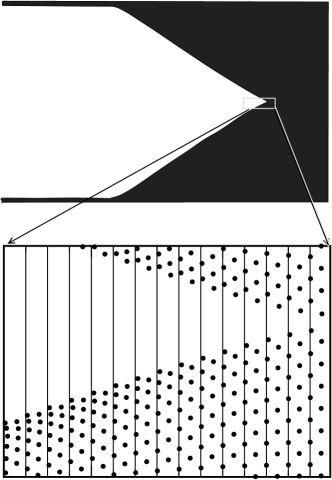
Figure 7: Snapshot of supersonic rupture in Neo–Hookean theory taken from numerical time evolution of Eq. (37). Note that particles do move almost purely vertically, as shown by comparing particle positions with the vertical lines.

The calculation of steady states for Eq. (37) is lengthy, and relegated to Appendix E. The final results are as follows:

Begin by specifying the dimensionless velocity and damping

$$\tilde{v}=v/c,\,\,\tilde{\beta}=\beta c/a,$$ (81)

and compute

$$\zeta=\frac{3-\cos(\omega/\tilde{v})-3\omega^{2}/[4(1-i\tilde{\beta}\omega)]}{2\cos(\omega/2\tilde{v})}$$ (82)

$$\phi=\zeta+\sqrt{\zeta^{2}-1}\mbox{with }\quad\textrm{abs}(\phi)>1,$$ (83)

$$F(\omega)=\left\{\frac{\phi^{[N-1]}-\phi^{-[N-1]}}{\phi^{N}-\phi^{-N}}-2\zeta\right\}\cos(\omega/2\tilde{v})+1,$$

$$\mbox{and}\quad Q(\omega) = \frac{F}{F-1-\cos(\omega/2\tilde{v})}.$$ (84)

Then the scaled extension $\tilde{\lambda}_{y}$ defined in Eq. (79) by $\tilde{\lambda_{y}}=\lambda_{y}/\sqrt{(4\lambda_{f}^{2}-\lambda_{x}^{2})/3}$ is given as a function of $\tilde{v}$ by

$$\tilde{\lambda}_{y} = \frac{1}{\sqrt{2N+1}}\exp\left[-\int\frac{d\omega^{\prime}}{4\pi}\left\{\frac{\left[\ln Q(\omega^{\prime})-\overline{\ln Q(\omega^{\prime})}\right]}{i\omega^{\prime}(1+\tilde{\beta}^{2}\omega^{\prime 2})}+\frac{\tilde{\beta}\ln|Q(\omega^{\prime})|^{2}}{1+\tilde{\beta}^{2}\omega^{\prime 2}}\right\}\right].$$ (85)

7 Results

7.1 Macroscopic Limit

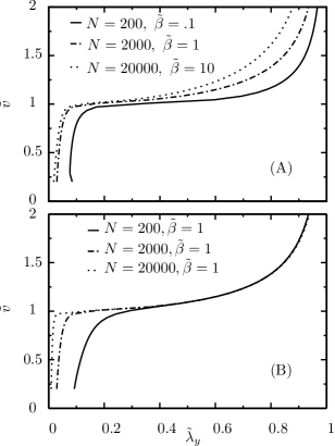
Figure 8: Sequence of velocity versus loading curves showing approaches to the continuum limit. Curves in (A) correspond to systems of fixed height and fixed continuum dissipation $\beta$, but sending the lattice spacing $a=L/N$ to zero. This is achieved through solutions of Eq. (85) where $N$ increases and $\tilde{\beta}=\beta c/a$ scales as $N.$ As $a$ goes to zero, the subsonic branch of solutions approaches a definite limiting value, but the velocity of supersonic solutions increases continually as $N$ increases. Note that on this approach to the continuum limit, the fracture energy diminishes as $a^{2}.$ Curves in (B) correspond to systems of fixed lattice spacing and fixed continuum dissipation $\beta$. As the height $L$ goes to infinity, the supersonic solutions approach a limiting value, but the branch of subsonic solutions is squeezed into a smaller and smaller region near the origin.

Eq. (85) provides a complete expression for the collection of extensions $\lambda_{x}$ and $\lambda_{y}$ that result in a rupture moving at velocity $v.$ Apart from the scaled velocity $\tilde{v}=v/c,$ the result depends upon three parameters; the system height $N$, the extension $\lambda_{f}$ at which bonds snap, and the coefficient of Kelvin dissipation $\tilde{\beta}=c\beta/a.$ One can now search for the conditions under which one should expect subsonic fractures, and the conditions under which one should expect supersonic ruptures. First, consider systems of fixed height and fixed level of dissipation $\beta$ as the lattice spacing tends to zero. This situation is described by fixing $L$ and taking the limit as $N\rightarrow\infty$ of Eq. (85) with $\tilde{\beta}=c\beta N/L$ also scaling as $N.$ Figure 8 (A) shows that in this limit, there is a narrow band of subsonic solutions followed by a broad band of supersonic solutions. Note that since the failure extension $\lambda_{f}$ remains fixed while the lattice spacing $a=L/N$ vanishes, the fracture energy vanishes as $a^{2}$ during this limiting procedure. Thus, this limiting procedure, which at first seems the most sensible, corresponds to something physically rather odd. Alternatively, one can set $\beta$ to a constant and send $N$ to $\infty$ so that the sample becomes infinitely high. In this limit, plotting solutions versus $\tilde{\lambda_{y}}$, the subsonic ruptures disappear, and only supersonic solutions survive, as shown in Fig. 8 (B). However, ones conclusions about the true nature of this macroscopic limit depend upon how one scales the solutions, as illustrated in Fig. 9. For a system of any given height, there are both subsonic and supersonic solutions. The subsonic solutions are found at small strain, and as $N$ becomes large, the range of extensions $\tilde{\lambda}_{y}$ that produces them becomes progressively smaller. There is a plateau near the wave speed that becomes wider and wider as $N$ increases. Finally, supersonic ruptures appear for extensions $\lambda_{y}$ on the order of $\lambda_{f}.$ The point to emphasize is that depending how extensions are scaled, either the supersonic or subsonic branches can be viewed as the macroscopic limit. In most brittle materials it is impossible for cracks to reach the wave speed because they become unstable to side-branching before this point is reached (Fineberg and Marder, 1999). One of the things that appears to make rubber different is that the ruptures are so stable that it is possible for them to pass the wave speed and move beyond it without instabilities intervening.

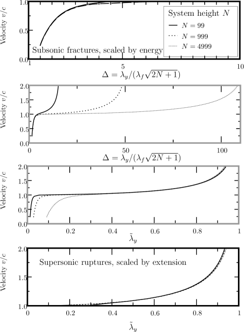
Figure 9: Four different views of Neo–Hookean crack velocities, showing that depending upon how they are scaled and displayed, one focuses either upon conventional subsonic fractures, or supersonic ruptures. The definition of $\tilde{\lambda_{y}}$ is given in Eq. (79). In the limit of infinite system height $N$, the two different types of solutions are separated by an infinitely long plateau at the wave speed.

7.2 Comparison with Experiment

To close this investigation, I compare the results with experiments on rupture of rubber sheets. It was already demonstrated in Figure 2 that the Mooney-Rivlin theory adequately captures the variation of sound speed with extension. The remaining two quantities measured by Petersan et al. (2004) are rupture speeds and opening angles. Before making the comparison, two reasons to view the comparison with a bit of skepticism should be noted. First, rubber is an entangled polymer network, not a triangular lattice. Second, although the Kelvin dissipation proportional to $\beta$ plays a very important role in the theory, no estimate of its value from experiment has been provided. The reason is that dissipation in real amorphous solids is not of the form employed here, nor is there any simple way to correct the deficiency. The spatial decay rate of sound waves in rubber over frequencies ranging from kilohertz to megahertz is almost perfectly linear in $\omega$ (Mott et al., 2002):

$$\alpha=C\omega,$$ (86)

where $C$ is a constant. However, given the form of Kelvin dissipation employed in this paper, sound decays at the rate

$$\alpha=\mbox{Im}(k)=\mbox{Im}\left[\omega/\left(c\sqrt{1-i\beta\omega}\right)\right].$$ (87)

It is impossible to find a value of $\beta$ that makes Eq. (87) a good fit to Eq. (86). A more realistic rule for Kelvin dissipation would provide a frequency-dependent sound speed according to

$$\frac{1}{c^{2}(\omega)}=\frac{1}{c_{\infty}^{2}}+\left(\frac{1}{c_{0}^{2}}-\frac{1}{c_{\infty}^{2}}\right)\frac{1}{1-i\beta\omega};$$ (88)

the form of dissipation used in Eq. (41) corresponds to sending to the high-frequency sound speed $c_{\infty}$ to infinity. However, the frequency dependence of sound attenuation does not resemble experiment any better after inclusion of $c_{\infty}.$ Thus I will simply continue to use the simplest form of Kelvin dissipation, as it is familiar and conventional (Fradkin et al., 2003) and take the dimensionless measure of dissipation, $\tilde{\beta}=\beta c/a$ to be of order unity. Fortunately, none of the final results depend much on the value of $\tilde{\beta}$.

Figure 10 assembles experimental and theoretical results. According to the theory for triangular lattices, samples with extensions $\lambda_{x}$ and $\lambda_{y}$ depend only upon the scaled variable $\tilde{\lambda}_{y}$ given by Eq. (79). This scaling of the velocity is compatible with all the data. Thirteen experimental trials where ruptures ran straight collapse onto five points, with rather little variation in the scaled velocity. The scatter in the data is rather large, and therefore consistent both with the simplified results of Section 5, as well as the more elaborate results of Section 6. The figure also shows a comparison of direct integration of the equations of motion, Eq. (33). For the equations of motion in this figure, the Mooney–Rivlin parameter $B$ has been set to zero, but $E_{zz}$ has not been eliminated from Eq. (17). Agreement with the analytical results from Eq. (85) is excellent, showing that details of how rubber relaxes behind the tip of the rupture do not have much effect on the dynamics. As already shown in Figure 5, rupture speeds are not measurably affected by including $B.$ Therefore, the analytical results of Eq. (85) capture rupture speeds, experimental and numerical, rather completely. The simple result of Eq. (79) is adequate for a first pass. In fact, the value $\lambda_{f}=5.5$ of the bond failure extension was obtained by fitting (79) to the experimental data, and this value of $\lambda_{f}$ was then used unchanged in all numerical runs.

Finally, Figure 11 compares experimental results for crack opening angles with predictions based upon numerical solutions of the most realistic numerical system, (33). That is, the nonlinear terms from $E_{zz}$ that appear as rubber shrinks towards its equilibrium relaxed state, and Rivlin’s nonlinear contribution to the Mooney-Rivlin energy are all included. Agreement between theory and experiment for the opening angle is still not completely satisfactory. The experimental points are widely scattered, indicating that the reduction to the variable $\tilde{\lambda_{y}}$ may not be appropriate, and experimental values lie systematically below theoretical predictions. Either the simplistic form of the dissipation, or the simplistic triangular microstructure might be to blame for this discrepancy.

There is one final potential discrepancy with experiment that should be mentioned. According to the theory, the dynamical solutions do include subsonic ruptures at small extensions. Many rubbers are well known to creep (Hui et al., 2003), and tear slowly in trouser tests, but in our biaxially loaded samples of natural latex rubber we never observed cracks to creep, or to travel slower than the sound speed at all.

Figure 10: Comparison of theory, experiment, and numerics for rubber rupture velocities. Experimental velocities are scaled by $c\lambda_{x}$, with $c=$22 m/s, while the vertical extension $\lambda_{y}$ is scaled by $\sqrt{(4\lambda_{f}^{2}-\lambda_{x}^{2})/3}$. The continuum approximation is given in Eq. (79). Direct integration of Eq. (33) is carried out in triangular lattices $N=$200 rows high in the Neo–Hookean limit where $B=0,$ with Kelvin dissipation $\beta=3,$ and retaining $E_{zz}$ as in Eq. (17). The Discrete Solution is an exact solution of the same system using the Wiener-Hopf technique,with the three differences. First, $E_{zz}$ is neglected in the analytical solution. Second, the analytical system is infinitely long in the horizontal direction, while the numerical system is finite. Third, in the numerical system there is a brief time when only one of two crack-line bonds has snapped, and horizontal forces on crack-line atoms do not balance to zero, while in the analytical solutions, all forces in the horizontal direction are ignored. Analytical solutions for systems both 200 and 2000 rows high are displayed to show how the continuum limit is achieved.

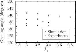
Figure 11: Rupture opening angles obtained from simulations and compared with experiment. The agreement is not very satisfactory; the experimental results are widely scattered, but lie systematically below the numerical predictions. For prediction of this quantity, it may be that treating rubber as a triangular lattice is not adequate.

8 Conclusions

The main points established by this theory for the rupture of rubber are the following:

1. The rupture of rubber is a shock phenomenon, with the back edges traveling at a wave speed, and the tip of the rupture consisting in the place where two shocks meet at a point.

2. The essential physical ingredients are dissipation and some toughening that allows the back end of the rupture to retain its integrity. Static hyperelasticity appears not to be relevant.

3. Predictions for rupture velocity are in satisfactory agreement with experiment. Predictions for opening angle are less so, perhaps because the computations have been performed in a triangular lattice, and with a very simple form of dissipation.

Additional physical question that have not yet been resolved are

1. Under what conditions do cracks in rubber creep, and when instead are they supersonic?

2. What is the origin of rupture path oscillations reported by Deegan et al. (2002)?

Appendix A Reduction to 2 dimensions

This Appendix shows in two different ways how to obtain an effective two-dimensional equation of motion for a rubber sheet. In the first, method, the incompressibility of rubber is used to calculate the thickness of the sheet at every point, thus expressing displacements across the thickness of the sheet ($z$ direction) in terms of the extensions along $x$ and $y$ (Figure 1).

A.1 First method

Rubber is highly incompressible, so one can set

$$\det\left|\frac{\partial\vec{u}}{\partial\vec{r}}\right|=0.$$ (89)

For a thin sheet, assume that one can neglect $\partial u^{y}/\partial z$ and $\partial u^{x}/\partial z$, on the grounds that $u^{x}$ and $u^{y}$ should be uniform through the thickness of the sheet. Then Eq. (89) becomes

$$\frac{\partial u^{z}}{\partial r_{z}}\left(\frac{\partial u^{x}}{\partial r_{x}}\frac{\partial u^{y}}{\partial r_{y}}-\frac{\partial u^{x}}{\partial r_{y}}\frac{\partial u^{y}}{\partial r_{x}}\right)=1.$$ (90)

Since $u^{x}$ and $u^{y}$ are assumed to be independent of $z$, one can write

$$u^{z}=r_{z}\,\left(\frac{\partial u^{x}}{\partial r_{x}}\frac{\partial u^{y}}{\partial r_{y}}-\frac{\partial u^{x}}{\partial r_{y}}\frac{\partial u^{y}}{\partial r_{x}}\right)^{-1}$$

which is odd in $r_{z}$ In moving to a two–dimensional theory, replace all quantities by their averages across the sheet. That is, if the sheet has thickness $t$ in the reference frame, then for example,

$$E_{xz}(r_{x},r_{y})\equiv\int_{-t/2}^{t/2}\frac{dr_{z}}{t}\,E_{xz}(r_{x},r_{y},r_{z}).$$ (91)

Consider now

$$E_{xz}(\vec{r})=\frac{1}{2}\left(\frac{\partial u^{x}}{\partial r_{x}}\frac{\partial u^{x}}{\partial r_{z}}+\frac{\partial u^{y}}{\partial r_{x}}\frac{\partial u^{y}}{\partial r_{z}}+\frac{\partial u^{z}}{\partial r_{x}}\frac{\partial u^{z}}{\partial r_{z}}\right).$$

To obtain the two–dimensional version of this quantity, note that the first two terms vanish because of the derivatives with respect to $r_{z}$ while the last term is odd in $r_{z}$, and vanishes when averaged across the sheet thickness in (91) . Therefore, in the two–dimensional theory, one can take $E_{xz}=E_{yz}=0.$ Finally, consider

$$E_{zz}=\frac{1}{2}\left(\left[\frac{\partial u^{z}}{\partial r_{z}}\right]^{2}-1\right)=\frac{1}{2}\left(\left(\frac{\partial u^{x}}{\partial r_{x}}\frac{\partial u^{y}}{\partial r_{y}}-\frac{\partial u^{x}}{\partial r_{y}}\frac{\partial u^{y}}{\partial r_{x}}\right)^{-2}-1\right).$$ (92)

The derivatives appearing in the denominator of (92) can be expressed in terms of the two–dimensional invariants in Eq. (7) as

$$E_{zz}=\frac{1}{2}\left(\frac{1}{4I_{2}+2I_{1}+1}-1\right),$$

which is Eq. (8).

A.2 Second Method

Specialize to the case of a Neo–Hookean material. Note that raised indices are employed on $u$ because elsewhere in the manuscript subscripts are needed to index the locations of multiple particles; raised indices are just ordinary Cartesian components of the vector $\vec{u}$. For an incompressible solid the Cauchy stress tensor is (Ogden, 1984)

$$T_{\alpha\beta}=\rho c^{2}\frac{\partial u^{\alpha}}{\partial r_{\gamma}}\frac{\partial u^{\beta}}{\partial r_{\gamma}}-p\delta_{\alpha\beta},$$ (93)

where $p$ is a pressure that must be determined by the condition of incompressibility. To find an equation of motion, one needs the Piola-Kirkhoff stress tensor, which for an incompressible material takes the form

$$S_{\alpha\beta}=\frac{\partial r_{\alpha}}{\partial u^{\lambda}}T_{\lambda\beta}=\rho c^{2}\frac{\partial u^{\beta}}{\partial r_{\alpha}}-p\frac{\partial r_{\alpha}}{\partial u^{\beta}}.$$ (94)

Writing out the equation of motion gives

$$\rho\frac{\partial^{2}u^{\alpha}}{\partial t^{2}}=\frac{\partial}{\partial r_{\lambda}}S_{\lambda\alpha}=\frac{\partial}{\partial r_{\lambda}}\left[\rho c^{2}\frac{\partial u^{\alpha}}{\partial r_{\lambda}}-p\frac{\partial r_{\lambda}}{\partial u^{\alpha}}\right].$$ (95)

From Eq. (90) one can write $\partial r_{\alpha}/\partial u^{\beta}$ as

$$\left(\begin{array}[]{cc}\frac{\partial r_{x}}{\partial u^{x}}&\frac{\partial r_{y}}{\partial u^{x}}\\ \frac{\partial r_{x}}{\partial u^{y}}&\frac{\partial r_{y}}{\partial u^{y}}\end{array}\right)=\left(\begin{array}[]{cc}\frac{\partial u^{x}}{\partial r_{x}}&\frac{\partial u^{y}}{\partial r_{x}}\\ \frac{\partial u^{x}}{\partial r_{y}}&\frac{\partial u^{y}}{\partial r_{y}}\end{array}\right)^{-1}=\frac{\partial u^{z}}{\partial r_{z}}\left(\begin{array}[]{cc}\frac{\partial u^{y}}{\partial r_{y}}&-\frac{\partial u^{y}}{\partial r_{x}}\\ -\frac{\partial u^{x}}{\partial r_{y}}&\frac{\partial u^{x}}{\partial r_{x}}\end{array}\right).$$ (96)

Now examine the equation of motion for $u^{x}$,

$$\rho\frac{\partial^{2}u^{x}}{\partial t^{2}}=\left(\frac{\partial}{\partial r_{\lambda}}\rho c^{2}\frac{\partial u^{\alpha}}{\partial r_{\lambda}}\right)-\frac{\partial}{\partial r_{x}}\left(p\frac{\partial u^{z}}{\partial r_{z}}\frac{\partial u^{y}}{\partial r_{y}}\right)+\frac{\partial}{\partial r_{y}}\left(p\frac{\partial u^{z}}{\partial r_{z}}\frac{\partial u^{y}}{\partial r_{x}}\right).$$ (97)

Compare this result with the one that would come by inserting the constraint at the outset: Using Eq. (92) one finds

$$\rho\frac{\partial^{2}u^{x}}{\partial t^{2}} = -\frac{\delta}{\delta u^{x}(\vec{r)}}\int d\vec{r}\>\rho c^{2}(E_{xx}+E_{yy}+E_{zz})$$

$$= \left(\frac{\partial}{\partial r_{\lambda}}\rho c^{2}\frac{\partial u^{\alpha}}{\partial r_{\lambda}}\right)-\frac{\partial}{\partial r_{x}}\left[\rho c^{2}\left(\frac{\partial u^{z}}{\partial r_{z}}\right)^{3}\frac{\partial u^{y}}{\partial r_{y}}\right]$$

$$\quad\quad\quad\quad\quad\quad\>\>+\frac{\partial}{\partial r_{y}}\left[\rho c^{2}\left(\frac{\partial u^{z}}{\partial r_{z}}\right)^{3}\frac{\partial u^{y}}{\partial r_{x}}\right]$$

Eqs. (97) and (A.2) are the same provided that

$$p=\rho c^{2}\left(\frac{\partial u^{z}}{\partial r_{z}}\right)^{2}.$$ (99)

Thus the equation of motion obtained by employing the constraint in Eq. (8) is compatible with the equation of motion one obtains from the Piola-Kirkhoff stress tensor so long as one uses Eq. (99) for the pressure. Furthermore, this expression for the pressure is precisely what is needed so that $T_{zz}$ vanishes in Eq. (93), and that in turn is what one would expect as the appropriate boundary condition for a thin sheet.

Appendix B Sound Speeds

Given an energy functional

$$U = \rho\int d\vec{r}\>e(I_{1},I_{2}),$$

where $\rho$ is the mass per area measured in the reference frame, the aim of this appendix is to calculate sound speeds. The same results are found for example in (Eringen and Suhubi, 1974, v. 1, pp. 120, 263), but to obtain the simple expressions for longitudinal and shear waves needed here, it may be easier to begin again than to work backwards through so much notation. To begin, find how $U$ varies when there is a small change in $u$:

$$\frac{1}{\rho}\frac{\delta U}{\delta u^{\gamma}(\vec{r})}=-\sum_{\alpha,\beta}\left[\frac{\partial^{2}u^{\gamma}}{\partial r_{\alpha}\partial r_{\beta}}\frac{\partial e}{\partial E_{\alpha\beta}}+\frac{1}{2}\left\{\frac{\partial u^{\gamma}}{\partial r_{\alpha}}\frac{\partial}{\partial r_{\beta}}+\frac{\partial u^{\gamma}}{\partial r_{\beta}}\frac{\partial}{\partial r_{\alpha}}\right\}\frac{\partial e}{\partial E_{\alpha\beta}}\right]$$

Take $\partial e/\partial E_{\alpha\beta}$ to be symmetric under interchange of $\alpha$ and $\beta$. This is only true if from now on whenever one sees $E_{xy}$ in some term in the free energy, one replaces it by $\left(E_{xy}+E_{yx}\right)$/2, and we will have to be careful to do that. However, assuming this symmetry, one can write

$$\frac{1}{\rho}\frac{\delta U}{\delta u^{\gamma}(\vec{r})} = -\sum_{\alpha,\beta}\left[\frac{\partial^{2}u^{\gamma}}{\partial r_{\alpha}\partial r_{\beta}}\frac{\partial e}{\partial E_{\alpha\beta}}+\sum_{\alpha^{\prime}\beta^{\prime}}\frac{\partial u^{\gamma}}{\partial r_{\alpha}}\frac{\partial E_{\alpha^{\prime}\beta^{\prime}}}{\partial r_{\beta}}\frac{\partial^{2}e}{\partial E_{\alpha\beta}\partial E_{\alpha^{\prime}\beta^{\prime}}}\right]$$

$$\!\!\!\!\!\!\!\ \!\!\!\!\!\!\!\ \!\!\!\!\!\!\!\ \!\!\!\!\!\!\!\ \!\!\!\!\!\!\!\ \!\!\!\!\!\!\!\ \!\!\!\!\!\!\!\ \!\!\!\!\!\!\!\ \!\!\!\!\!\!\!\ \!\!\!\!\!\!\!\ =-\sum_{\alpha,\beta}\left[\frac{\partial^{2}u^{\gamma}}{\partial r_{\alpha}\partial r_{\beta}}\frac{\partial e}{\partial E_{\alpha\beta}}+\sum_{\alpha^{\prime}\beta^{\prime}\gamma^{\prime}}\frac{1}{2}\frac{\partial u^{\gamma}}{\partial r_{\alpha}}\left({\displaystyle\frac{\partial}{\partial r_{\beta}}\left[\frac{\partial u^{\gamma^{\prime}}}{\partial r_{\alpha^{\prime}}}\frac{\partial u^{\gamma^{\prime}}}{\partial r_{\beta^{\prime}}}\right]}\right)\frac{\partial^{2}e}{\partial E_{\alpha\beta}\partial E_{\alpha^{\prime}\beta^{\prime}}}\right]$$

$$=-\sum_{\alpha,\beta}\left[\frac{\partial^{2}u^{\gamma}}{\partial r_{\alpha}\partial r_{\beta}}\frac{\partial e}{\partial E_{\alpha\beta}}+\sum_{\alpha^{\prime}\beta^{\prime}\gamma^{\prime}}\frac{\partial u^{\gamma}}{\partial r_{\alpha}}\frac{\partial u^{\gamma^{\prime}}}{\partial r_{\alpha^{\prime}}}\frac{\partial^{2}u^{\gamma^{\prime}}}{\partial r_{\beta^{\prime}}\partial r_{\beta}}\frac{\partial^{2}e}{\partial E_{\alpha\beta}\partial E_{\alpha^{\prime}\beta^{\prime}}}\right]$$

Now take $u$ to represent a sheet loaded up in biaxial strain, and superpose a small amplitude wave with polarization $\vec{\epsilon}$ traveling with wave vector $\vec{k}$. Take $\lambda_{\gamma}$to be the extension factor along direction $\gamma$, and $r_{\gamma}$ to be a position coordinate in the material frame. Keep only terms of order $\epsilon$. Inserting such a plane wave into Eq. (B), the result is

$$\frac{1}{\rho}\frac{\delta U}{\delta u^{\gamma}(\vec{r)}} \approx \sum_{\alpha,\beta}\left[k_{\alpha}k_{\beta}\epsilon_{\gamma}\frac{\partial e}{\partial E_{\alpha\beta}}+\sum_{\alpha^{\prime}\beta^{\prime}\gamma^{\prime}}\lambda_{\gamma}\delta_{\gamma\alpha}\>\lambda_{\gamma^{\prime}}\delta_{\gamma^{\prime}\alpha^{\prime}}k_{\beta^{\prime}}k_{\beta}\epsilon_{\gamma^{\prime}}\frac{\partial^{2}e}{\partial E_{\alpha\beta}\partial E_{\alpha^{\prime}\beta^{\prime}}}\right]$$ (101)

$$= \sum_{\alpha,\beta}\left[k_{\alpha}k_{\beta}\epsilon_{\gamma}\frac{\partial e}{\partial E_{\alpha\beta}}\right]+\left[\sum_{{{\beta\atop\beta^{\prime}\gamma}}}\lambda_{\gamma}\>\lambda_{\gamma^{\prime}}k_{\beta^{\prime}}k_{\beta}\epsilon_{\gamma^{\prime}}\frac{\partial^{2}e}{\partial E_{\gamma\beta}\partial E_{\gamma^{\prime}\beta^{\prime}}}\right]$$

$$= \sum_{\beta\beta^{\prime}\gamma^{\prime}}\left[k_{\beta}k_{\beta^{\prime}}\epsilon_{\gamma}\frac{\partial e}{\partial E_{\beta\beta^{\prime}}}+\lambda_{\gamma}\>\lambda_{\gamma^{\prime}}k_{\beta^{\prime}}k_{\beta}\epsilon_{\gamma^{\prime}}\frac{\partial^{2}e}{\partial E_{\gamma\beta}\partial E_{\gamma^{\prime}\beta^{\prime}}}\right]$$

$$= \sum_{\beta\beta^{\prime}\gamma^{\prime}}\left[\delta_{\gamma\gamma^{\prime}}\frac{\partial e}{\partial E_{\beta\beta^{\prime}}}+\lambda_{\gamma}\lambda_{\gamma^{\prime}}\frac{\partial^{2}e}{\partial E_{\gamma\beta}\partial E_{\gamma^{\prime}\beta^{\prime}}}\right]k_{\beta^{\prime}}k_{\beta}\epsilon_{\gamma^{\prime}}.$$

Therefore, one has an equation of motion for sound waves

$$\rho\omega^{2}\epsilon_{\gamma} = \frac{\delta U}{\delta u^{\gamma}(\vec{r})}$$

$$\Rightarrow\omega^{2}\epsilon_{\gamma} = \sum_{\gamma^{\prime}\beta\beta^{\prime}}\left[\delta_{\gamma\gamma^{\prime}}\frac{\partial e}{\partial E_{\beta\beta^{\prime}}}+\lambda_{\gamma}\lambda_{\gamma^{\prime}}\frac{\partial^{2}e}{\partial E_{\gamma\beta}\partial E_{\gamma^{\prime}\beta^{\prime}}}\right]k_{\beta}k_{\beta^{\prime}}\epsilon_{\gamma^{\prime}}.$$ (102)

B.1 Specific expressions for longitudinal and shear waves

Take $\vec{k}=k(1,0)$. Assume that

$$\frac{\partial^{2}e}{\partial E_{xx}\partial E_{xy}}=\frac{\partial^{2}e}{\partial E_{yy}\partial E_{xy}}=0.$$ (103)

This will always be the case in biaxial strain just so long as the energy only depends upon strain through the combinations in $I_{1}$ and $I_{2}$. Longitudinal waves are found by looking for a wave polarized along $x$, which means that only $\epsilon_{x}$ is nonzero, so $\gamma=\gamma^{\prime}=x$. Note in addition that in Eq. (102) one can have $k_{\beta}=k_{\beta^{\prime}}=1$ only if $\beta=\beta^{\prime}=x$. Therefore

$$c_{lx}^{2}=\frac{\partial e}{\partial E_{xx}}+\lambda_{x}^{2}\frac{\partial^{2}e}{\partial E_{xx}^{2}}.$$ (104)

Next look for a wave polarized along $y.$ Now $\gamma=\gamma^{\prime}=y$. One still has to have $\beta=\beta^{\prime}=x$. Therefore for shear waves

$$c_{sx}^{2}=\frac{\partial e}{\partial E_{xx}}+\lambda_{y}^{2}\frac{\partial^{2}e}{\partial E_{xy}^{2}}\>\mbox{Assuming symmetry}$$ (105)

It is easy to use Eq. 105 improperly. It is only valid if $e$ is treated as a symmetrical function of $E_{xy}$ and $E_{yx}$, and if partial derivatives with respect to these two quantities are independent. It is hard to remember to retain this convention, and it is safer simply to set $E_{xy}=E_{yx}$ and treat $e$ just as a function of one of them. In this case, one must write

$$c_{sx}^{2}=\frac{\partial e}{\partial E_{xx}}+\frac{\lambda_{y}^{2}}{4}\frac{\partial^{2}e}{\partial E_{xy}^{2}}.$$ (106)

The analogous expressions for wave speeds along $y$ follow by flipping the roles of $x$ and $y$.

The expressions for sound speeds take much simpler forms if one establishes spatially uniform states in the rubber and considers small uniform disturbances. Return to Eqs. (15a) and (15b). Establish the displacement field

$$\vec{u}=(\lambda_{x}x+s_{xy}y,\lambda_{y}y+s_{yx}x).$$ (107)

Specialize now to the case where a sample is subject to uniform bi–axial strain, and sheared in the $y$ direction, so that $s_{xy}$ is zero. Then inserting Eq. (107) into Eq. 5 gives

$$E_{xx} = {\textstyle\frac{1}{2}}\left(\lambda_{x}^{2}+s_{yx}^{2}-1\right)$$ (108)

$$E_{yy} = {\textstyle\frac{1}{2}}\left(\lambda_{y}^{2}-1\right)$$ (109)

$$E_{xy} = {\textstyle E_{yx}=\frac{1}{2}}\lambda_{y}s_{yx}$$ (110)

Derivatives with respect to components of the strain tensor can all now be expressed in terms of the new variables $\lambda_{x}$, $\lambda_{y}$, and $s_{yx}$. Since these variables correspond exactly to quantities one controls experimentally, it is good to express sound speeds in terms of them. One has

$$\frac{\partial\left\{E_{xx}E_{yy}E_{xy}\right\}}{\partial\left\{\lambda_{x}\lambda_{y}s_{yx}\right\}}=\left(\begin{array}[]{ccc}\lambda_{x}&0&s_{yx}\\ 0&\lambda_{y}&0\\ 0&s_{yx}/2&\lambda_{y}/2\end{array}\right).$$ (111)

Inverting this matrix, one has

$$\frac{\partial\left\{\lambda_{x}\lambda_{y}s_{yx}\right\}}{\partial\left\{e_{xx}e_{yy}e_{xy}\right\}}=\left(\begin{array}[]{ccc}\frac{1}{\lambda_{x}}&\frac{s_{yx}^{2}}{\lambda_{x}\lambda_{y}^{2}}&-\frac{2s_{yx}}{\lambda_{x}\lambda_{y}}\\ 0&\frac{1}{\lambda_{y}}&0\\ 0&-\frac{s_{yx}}{\lambda_{y}^{2}}&\frac{2}{\lambda_{y}}\end{array}\right).$$ (112)

Therefore, one can write

$$\frac{\partial}{\partial E_{xx}} = \frac{1}{\lambda_{x}}\frac{\partial}{\partial\lambda_{x}}$$ (113)

$$\frac{\partial}{\partial E_{xy}} = -\frac{2s_{yx}}{\lambda_{y}\lambda_{y}}\frac{\partial}{\partial\lambda_{x}}+\frac{2}{\lambda_{y}}\frac{\partial}{\partial s_{yx}}.$$ (114)

Inserting Eq. (113) into Eq. (15a) and Eq. (114) into Eq. (15b) and evaluating at $s_{yx}=0$ gives Eqs. (3.2).

Appendix C Force computation

I record here some methods used to calculate forces in molecular dynamics that assist in writing computer code, and that may not have been published previously. The force on component $\alpha$ of particle $l$ is defined to be

$$F_{l}^{\alpha}\equiv-\frac{\partial U}{\partial u_{l}^{\alpha}}.$$ (115)

For the purposes of writing computer code, it is not efficient to proceed directly with this expression, because in the course of computing, say, $F_{1}$ one might calculate some quantities that will also appear in $F_{2}$ and efficient code will duplicate as little computation as possible. Therefore, define the insertion operator $\mathcal{I}_{l}$. Any term that is multiplied by $\mathcal{I}_{l}$ is to be inserted into the memory location that holds the force on particle $l$. So one computes

$$\sum_{l}F_{l}^{\alpha}I_{l}/m=-\sum_{li}\mathcal{I}_{l}\left[\frac{\partial w}{\partial I_{1}^{i}}\frac{\partial I_{1}^{i}}{\partial u_{l}^{\alpha}}+\frac{\partial w}{\partial I_{2}^{i}}\frac{\partial I_{2}^{i}}{\partial u_{l}^{\alpha}}\right]$$ (116)

Thus one must compute a sum of two terms. The first is

$$\sum_{li,j\in n(i)}\mathcal{I}_{l}\frac{\partial w}{\partial I_{1}^{i}}\frac{1}{3a^{2}}(\delta_{il}-\delta_{jl})u_{ij}^{\alpha}=\sum_{i,j\in n(i)}(\mathcal{I}_{i}-\mathcal{I}_{j})\frac{\partial w}{\partial I_{1}^{i}}\frac{1}{3a^{2}}u_{ij}^{\alpha}$$ (117)

(but this term vanishes if $u_{ij}>a\lambda_{f}$)

The second is

$$\sum_{ij\in n(i)}(\mathcal{I}_{i}-\mathcal{I}_{j})u_{ij}^{\alpha}\frac{\partial w}{\partial J_{2}^{i}}\frac{3}{4a^{4}}\left[\frac{2}{3}F_{i}-\frac{4}{9}(\vec{u}_{ij}\cdot\vec{u}_{ij}-a^{2})\right],$$ (118)

(but vanish if $u_{ij}>a\lambda_{f})$ or, if one takes the alternate representation of $I_{2}^{i},$

$$\sum_{ij\in n(i)}(\mathcal{I}_{i}-\mathcal{I}_{j})u_{ij}^{\alpha}\frac{\partial w}{\partial I_{2}^{i}}\frac{9}{8a^{4}}\left[\frac{4}{9}(\vec{u}_{ij}\cdot\vec{u}_{ij}-a^{2})\right]+\sum_{l}\mathcal{I}_{l}\frac{\partial w}{\partial I_{2}^{i}}\frac{9}{8a^{4}}\frac{\partial H_{i}}{\partial u_{l}^{\alpha}},$$ (119)

The final term to compute is (with $g_{ijk}\equiv(\vec{u}_{ij}\cdot\vec{u}_{ik}+2a^{2})^{2})$

$$H_{i}\equiv\frac{1}{27}\sum_{j\neq k\in n(i)}(\vec{u}_{ij}\cdot\vec{u}_{ik}+2a^{2})^{2}h(u_{ij})h(u_{ik})\equiv\frac{1}{27}\sum_{j\neq k\in n(i)}g_{ijk}h_{ij}h_{ik}$$ (120)

and derivatives of this object contribute to the force

$$-\sum_{{{i\atop j\neq k\in n(i)}}}\frac{\partial w}{\partial J_{2}^{i}}\frac{1}{27}\frac{9}{8a^{4}}\left\{\begin{array}[]{cc}&h^{\prime}_{ij}h_{ik}g_{ijk}\frac{u_{ij}^{\alpha}}{u_{ij}}\left(\mathcal{I}_{i}-\mathcal{I}_{j}\right)+h^{\prime}_{ik}h_{ij}g_{ijk}\frac{u_{ik}^{\alpha}}{u_{ik}}\left(\mathcal{I}_{i}-\mathcal{I}_{k}\right)\\ \vskip 0.0pt\cr\\ +&h{}_{ij}h_{ik}g^{\prime}_{ijk}\left(\mathcal{I}_{i}\left\{u_{ij}^{\alpha}+u_{ik}^{\alpha}\right\}-\mathcal{I}_{k}u_{ij}^{\alpha}-\mathcal{I}_{j}u_{ik}^{\alpha}\right)\end{array}\right\}.$$ (121)

Note in all these expression that various quantities need only be computed once and inserted into registers for particles $i$, $j,$ and $k.$ The insertion operators $\mathcal{I}_{i}$ , $\mathcal{I}_{j}$ , and $\mathcal{I}_{k}$ keep track of which quantities to put where.

Appendix D Lattice Instabilities

I found numerically that when I employed Eq. (28), the uniformly strained lattice would spontaneously develop a striped pattern when stretched beyond a critical value. To analyze this problem, I computed the phonon dynamical matrix (Marder, 2000, Eq. 13.8, p. 307). The calculation is a straightforward exercise in phonon physics, and no details need to be reported. Negative eigenvalues of this matrix indicate instability of the uniform state. As shown in Figure 12, for uniform biaxial strain a bit above $\lambda_{x}=\lambda_{y}=3,$ the spatially uniform lattice becomes unstable. However, if one employs instead Eq. (29), then as shown in Fig. 13, the lattice remains stable. For this reason, Eq. (29) was usually employed, despite its greater numerical cost. It would be interesting to see whether the instability in Fig. 12 is related to strain crystallization.

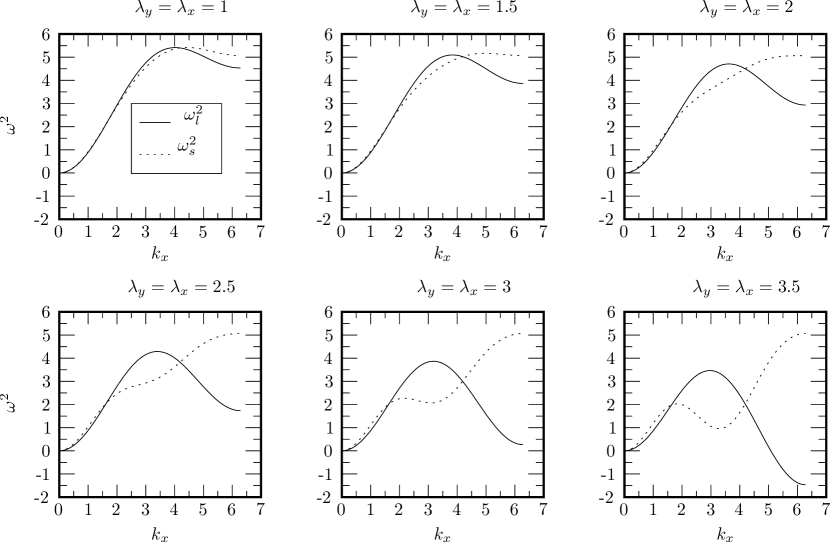
Figure 12: Frequency squared as a function of wave number for various levels of uniform biaxial strain, using the energy potential function in Eq. (28). As the strain increases, the lattice becomes unstable to a distortion in which every other column of atoms moves in opposite directions, similar to motions of atoms in optical modes, or the Peierls distortion.

Figure 13: Frequency squared as a function of wave number for various levels of uniform biaxial strain, using the energy potential function in Eq. (29). With this representation of the strain invariant, the uniform lattice remains stable against high-frequency distortions over the range of extensions employed experimentally.

Appendix E Solution of Discrete System

This Appendix contains the steady-state solution of

$$\ddot{u}_{i}^{\alpha}=\frac{2c^{2}}{3a^{2}}\sum_{j\in n(i)}\left(u_{ij}^{\alpha}+\beta\dot{u}_{ij}^{\alpha}\right)\theta(\lambda_{f}-u_{ij}).$$ (122)

The methods employed are those of Slepyan (1981, 1982, 2002); see also (Marder and Gross, 1995; Marder, 2004). Slepyan (2002, p. 478) notes the existence of supersonic solutions for a related problem. However, the steps below are worth recording in detail because the particular combination of Kelvin viscosity, Mode III, and a strip of finite height needed here has not been published, although no especially new ideas are involved.

Move to notation that explicitly describes locations in a triangular lattice, $u(m,n),$ where $u$ describes the vertical motion of atoms only, since the horizontal motion is neglected, and where $m\in(-\infty\dots-3,-2,-1,0,1,2,3,\dots\infty)$ and $n\in(\dots-5/2,\ -3/2,\ -1/2,\ 1/2,\ \ 3/2,\ 5/2\dots$. Then in steady state, one has the symmetries

$$u(m,n,t) = u(m+1,n,t+a/v)$$ (123)

$$u(m,n,t) = -u(m,-n,t-a[1/2-g_{n}]/v)$$ (124)

$$u(m,1/2,t) = -u(m,-1/2,t-a/2v),$$ (125)

where

$$g_{n} = \begin{cases}1&\textrm{if }n=3/2,\ 7/2...\\ 0&,\textrm{if }n=1/2,\ 5/2...\end{cases}$$ (126)

Assuming that a crack is in steady state, we can therefore eliminate the variable $m$ entirely from the equation of motion, by defining

$$u_{n}(t)=u(0,n,t).$$ (127)

Next, define dimensionless variables

$$\tilde{t}=tc/a;\ \tilde{\beta}=\beta c/a,\quad\mbox{and}\ \tilde{v}=v/c.$$ (128)

Then

$$\ddot{u}_{n}(\tilde{t}) = \frac{2}{3}(1+\tilde{\beta}\frac{\partial}{\partial\tilde{t}})\left[\begin{array}[]{lcl}+u_{n+1}(\tilde{t}-(g_{n+1}-1)/\tilde{v})&&+u_{n+1}(\tilde{t}-g_{n+1}/\tilde{v})\\ +u_{n}(\tilde{t}+1/\tilde{v})&-6u_{n}(\tilde{t})&+u_{n}(\tilde{t}-1/\tilde{v})\\ +u_{n-1}(\tilde{t}-(g_{n-1}-1)/\tilde{v})&&+u_{n-1}(\tilde{t}-g_{n-1}/\tilde{v})\end{array}\right]$$

if $$n>1/2$$ and

$$\ddot{u}_{1/2}(\tilde{t})=\frac{2}{3}\left[\begin{array}[]{lcl}+(1+\tilde{\beta}\frac{\partial}{\partial\tilde{t}})u_{3/2}(\tilde{t})+(1+\tilde{\beta}\frac{\partial}{\partial\tilde{t}})u_{3/2}(\tilde{t}-1/\tilde{v})\\ +(1+\tilde{\beta}\frac{\partial}{\partial\tilde{t}})\left[u_{1/2}(\tilde{t}+1/\tilde{v})-4u_{1/2}(\tilde{t})+u_{1/2}(\tilde{t}-1/\tilde{v})\right]\\ +\theta(-\tilde{t})(1+\tilde{\beta}\frac{\partial}{\partial\tilde{t}})[u_{-1/2}(\tilde{t})-u_{1/2}(\tilde{t})]\\ +\theta(1/(2\tilde{v})-\tilde{t})(1+\tilde{\beta}\frac{\partial}{\partial\tilde{t}})[u_{-1/2}(\tilde{t}-1/\tilde{v})-u_{1/2}(\tilde{t})]\end{array}\right]$$ (130)

if $n=1/2$.

The time at which the bond between $u(0,1/2,\tilde{t})$ and $u(0,-1/2,\tilde{t})$ breaks has been chosen to be $t=0$, so that by symmetry the time the bond between $u(0,1/2,\tilde{t})$ and $u(1,-1/2,\tilde{t})$ breaks is $1/2\tilde{v}$.

Above the crack line, the equations of motion are completely linear, so it is simple to find the motion of every atom with $n>1/2$ in terms of the behavior of an atom with $n=1/2$. Fourier transforming in time gives

$$-\omega^{2}u_{n}(\omega)=\frac{2}{3}(1-i\tilde{\beta}\omega)\left[\begin{array}[]{lll}&u_{n+1}(\omega)&[e^{i\omega(g_{n+1}-1)/\tilde{v}}+e^{i\omega(g_{n+1})/\tilde{v}}]\\ +&u_{n}(\omega)&[e^{i\omega/\tilde{v}}-6+e^{-i\omega/\tilde{v}}]\\ +&u_{n-1}(\omega)&[e^{i\omega(g_{n-1}-1)/\tilde{v}}+e^{i\omega(g_{n-1})/\tilde{v}}]\end{array}.\right]$$ (131)

Let

$$u_{n}(\omega)=u_{1/2}(\omega)e^{k(n-1/2)-i\omega g_{n}/(2\tilde{v})}.$$ (132)

Substituting Eq. (132) into Eq. (131), and noticing that $g_{n}+g_{n+1}=1$ gives

$$-\omega^{2}u_{1/2}(\omega)=(1-i\tilde{\beta}\omega)\frac{2}{3}\left[\begin{array}[]{lll}&u_{1/2}(\omega)e^{k}&[e^{i\omega(g_{n+1}+g_{n-2})/(2\tilde{v})}+e^{i\omega(g_{n+1}+g_{n})/(2\tilde{v})}]\\ +&u_{1/2}(\omega)&[e^{i\omega/\tilde{v}}-6+e^{-i\omega/\tilde{v}}]\\ +&u_{1/2}(\omega)e^{-k}&[e^{i\omega(g_{n-1}+g_{n-2})/(2\tilde{v})}+e^{i\omega(g_{n-1}+g_{n})/(2\tilde{v})}]\end{array}\right]$$ (133)

$$\Rightarrow\frac{\omega^{2}}{1-i\tilde{\beta}\omega}+\frac{4}{3}\left[2\cosh(k)\cos(\omega/(2\tilde{v}))+\cos(\omega/\tilde{v})-3\right]=0.$$ (134)

Defining

$$\zeta=\frac{3-\cos(\omega/\tilde{v})-3\omega^{2}/[4(1-i\tilde{\beta}\omega)]}{2\cos(\omega/2\tilde{v})}$$ (135)

one has equivalently that

$$\phi=e^{k}=\zeta+\sqrt{\zeta^{2}-1}\ \mbox{\ \ with }\quad\textrm{abs}(\phi)>1.$$ (136)

One can construct a solution which meets all the boundary conditions by writing

$$u_{n}(\omega) = u_{1/2}(\omega)e^{-i\omega g_{n}/2\tilde{v}}[\frac{\phi^{[N+1/2-n]}-\phi^{-[N+1/2-n]}}{\phi^{N}-\phi^{-N}}]$$ (137)

$$+ \frac{U_{N}(n-1/2)}{N}\frac{2\epsilon}{\epsilon^{2}+\omega^{2}}.$$

This solution equals $u_{1/2}$ for $n=1/2$, and equals $U_{N}2\epsilon/(\epsilon^{2}+\omega^{2})$ for $n=N+1/2$. The reason to introduce $\epsilon$ is that for $n=N+1/2$, $u(m,n,t)=U_{N}$. The Fourier transform of this boundary condition is a delta function, and hard to work with formally. To resolve uncertainties, it is better to use instead the boundary condition

$$u_{N+1/2}(t)=U_{N}e^{-\epsilon|t|},$$ (138)

and send $\epsilon$ to zero the end of the calculation. In what follows, frequent use will be made of the fact that $\epsilon$ is small.

The most interesting variable is not $u_{1/2}$, but the distance between the bonds which will actually snap. Furthermore, the quantity multiplied by the $\theta$ function in Eq. 130 is operated upon by $(1+\beta\partial/\partial t)$ since dissipation stops operating when bonds break. For this reason define

$$U(t)={\frac{u_{1/2}(t)-u_{-1/2}(t)}{2}}={\frac{u_{1/2}(t)+u_{1/2}(t+1/2v)}{2}}.$$ (139)

$$W(\tilde{t})=(1+\tilde{\beta}\frac{\partial}{\partial\tilde{t}})U(\tilde{t})$$

Rewrite 130 as

$$\ddot{u}_{1/2}(\tilde{t})=\frac{2}{3}\left[\begin{array}[]{lr}+(1+\tilde{\beta}\frac{\partial}{\partial\tilde{t}})u_{3/2}(\tilde{t})+(1+\tilde{\beta}\frac{\partial}{\partial t})u_{3/2}(\tilde{t}-1/\tilde{v})\\ \vskip-7.22743pt\cr\\ +(1+\tilde{\beta}\frac{\partial}{\partial\tilde{t}})\left(u_{1/2}(\tilde{t}+1/\tilde{v})-4+u_{1/2}(\tilde{t})+u_{1/2}(\tilde{t}-1/\tilde{v})\right)\\ \vskip-7.22743pt\cr\\ -2U(\tilde{t})\theta(-\tilde{t})-2U(\tilde{t}-1/2\tilde{v})\theta(1/(2\tilde{v})-\tilde{t})\end{array}\right].$$ (140)

Fourier transforming this expression using Eq. (137) and defining

$$U^{\pm}(\omega)=\int_{-\infty}^{\infty}d\tilde{t}\,e^{i\omega\tilde{t}}U(\tilde{t})\theta(\pm\tilde{t}),$$ (141)

$$W^{\pm}(\omega)=\int_{-\infty}^{\infty}d\tilde{t\,}e^{i\omega\tilde{t}}W(\tilde{t})\theta(\pm\tilde{t}),$$ (142)

now gives

$$(1-i\omega\tilde{\beta})u_{1/2}(\omega)F(\omega)-(1+e^{i\omega/2\tilde{v}})U^{-}(\omega)=-\frac{U_{N}}{N}\frac{2\epsilon}{\omega^{2}+\epsilon^{2}},$$ (143)

with

$$F(\omega)=\left\{\frac{\phi^{[N-1]}-\phi^{-[N-1]}}{\phi^{N}-\phi^{-N}}-2\zeta\right\}\cos(\omega/2\tilde{v})+1$$ (144)

Next, use Eq. (139)in the form

$$W(\omega)=(1-i\omega\tilde{\beta}){\frac{(1+e^{-i\omega/2\tilde{v}})}{2}}u_{1/2}(\omega)$$ (145)

to obtain

$$W(\omega)F(\omega)-2(\cos^{2}\omega/4\tilde{v})U^{-}(\omega)=-\frac{U_{N}}{N}\frac{2\epsilon}{\omega^{2}+\epsilon^{2}}.$$ (146)

Writing

$$W(\omega)=W^{+}(\omega)+W^{-}(\omega)$$ (147)

finally gives

$$W^{+}(\omega)Q(\omega)+W^{-}(\omega)={U_{N}Q_{0}}\left[{\frac{1}{\epsilon+i\omega}}+{\frac{1}{\epsilon-i\omega}}\right],$$ (148)

with

$$Q = F/(F-1-\cos(\omega/2\tilde{v})).$$ (149)

The Wiener-Hopf technique (Noble, 1958) directs one to write

$$Q(\omega)={\frac{Q^{-}(\omega)}{Q^{+}(\omega)}},$$ (150)

where $Q^{-}$ is free of poles and zeroes in the lower complex $\omega$ plane and $Q^{+}$ is free of poles and zeroes in the upper complex plane. One can carry out this decomposition with the explicit formula

$$Q^{\pm}(\omega) = \exp[\lim_{\epsilon\rightarrow 0}\int{\frac{d\omega^{\prime}}{2\pi}}{\frac{\ln Q(\omega^{\prime})}{i\omega\mp\epsilon-i\omega^{\prime}}}].$$ (151)

Separate Eq. (148) into two pieces, one of which has poles only in the lower half plane, and one of which has poles only in the upper half plane:

$$\frac{W^{+}(\omega)}{Q^{+}(\omega)}-\frac{Q_{0}U_{N}}{Q(0)}\frac{1}{(-i\omega+\epsilon)}=\frac{Q_{0}U_{N}}{Q^{-}(0)}\frac{1}{(i\omega+\epsilon)}-\frac{W^{-}(\omega)}{Q^{-}(\omega)}.$$ (152)

Because the right and left hand sides of this equation have poles in opposite sections of the complex plane, they must separately equal a constant, ${\mathcal{C}}$. The constant must vanish, or $U^{-}$ and $U^{+}$ will behave as a delta function near $t=0$. So

$$W^{-}(\omega)=U_{N}\frac{Q_{0}Q^{-}(\omega)}{Q^{-}(0)(\epsilon+i\omega)}, W^{+}(\omega)=U_{N}\frac{Q_{0}Q^{+}(\omega)}{Q^{-}(0)(\epsilon-i\omega)}.$$ and (153)

One now has an explicit solution for $W(\omega)$. Numerical evaluation of $W(t)$ from Eq. (153) is fairly straightforward, using fast Fourier transforms. The most interesting quantity to obtain is the separation between bonds opposite the crack line at $t=0,$ since by setting this quantity so that the bond snaps, one obtains a consistent equation of motion. So one wants to find $U(0).$ To obtain it, write

$$U(\omega)=\frac{W^{+}(\omega)+W^{-}(\omega)}{1-i\tilde{\beta}\omega}.$$ (154)

The denominator of Eq. (154) has a pole in the lower half plane at

$$\omega=-i/\tilde{\beta}\equiv-i\omega_{0}$$ (155)

and this pole must be subtracted off in order to form $U^{-}.$ So one has

$$U^{-}(\omega)=\frac{W^{-}(\omega)-W^{-}(-i\omega_{0})}{1-i\tilde{\beta}\omega}.$$ (156)

In order to find $U(t=0)$ it is sufficient to find

$$U(t=0)=\lim_{\omega\rightarrow\infty}i\omega U^{-}(\omega).$$

The reason is that $U^{-}(t)$ is zero for all positive $t,$ dropping to zero right at $t=0.$ The value of $U(t=0)$ is given by the discontinuity in $U^{-}(t).$ However, if $U^{-}(\omega)$ decays faster than $1/\omega$ for large $\omega,$ then the inverse Fourier transform of $U^{-}(\omega)$ must be continuous at $t=0.$ Therefore, from the coefficient of $1/i\omega,$ one can pick out the value of $U(t=0).$ Since $W^{-}(t)$ like $U^{-}(t)$ has a step-function discontinuity at $t=0,$ $W^{-}(\omega)$ decays as $1/i\omega$ as $\omega$ goes to infinity. Thus one deduces immediately from (156) that

$$U(t=0)=\omega_{0}W^{-}(-i\omega_{0}).$$ (157)

Returning to (153) one has

$$U_{0}\equiv U(t=0)=U_{N}\frac{Q_{0}Q^{-}(-i\omega_{0})}{Q^{-}(0)}.$$ (158)

Note that the height of the top of the system $U_{N}$ obeys

$$\frac{\sqrt{3}}{2}a(N+1/2)\lambda_{y}=U_{N},$$

and that $Q_{0}=Q(0)=1/(2N+1)$ so

$$U_{0}=\frac{\sqrt{3}}{4}a\lambda_{y}\frac{Q^{-}(-i\omega_{0})}{Q^{-}(0)}.$$

The condition for a bond to snap is that the total length of the bond reach $a\lambda_{f}$. Note from the definition in Eq. (139) that $U$ gives only half the bond length. Therefore

$$\lambda_{f}^{2} = \frac{1}{4}\lambda_{x}^{2}+\frac{(2U_{0})^{2}}{a^{2}}$$

$$\Rightarrow 2U_{0} = a\sqrt{(\lambda_{f}^{2}-\lambda_{x}^{2}/4)}=\frac{\sqrt{3}}{2}a\lambda_{y}\frac{Q^{-}(-i\omega_{0})}{Q^{-}(0)}$$

$$\Rightarrow\frac{\lambda_{y}}{\sqrt{(4\lambda_{f}^{2}-\lambda_{x}^{2})/3}}=\frac{Q^{-}(0)}{Q^{-}(-i\omega_{0})}.$$

Employing (151) to obtain an explicit representation of $Q^{-}$ leads to Eq. (85).

References

- Atkin and Fox (1980) Atkin, R. J., Fox, N., 1980. An Introduction to the Theory of Elasticity. Longman, London.
- Broberg (1999) Broberg, K. B., 1999. Cracks and Fracture. Academic Press, San Diego.
- Buehler et al. (2003) Buehler, M. J., Abraham, F. F., Gao, H., 2003. Hyperelasticity governs dynamic fracture at a critical length scale. Nature 426, 141–146.
- Deegan et al. (2002) Deegan, R. D., Petersan, P., Marder, M., Swinney, H. L., 2002. Oscillating fracture paths in rubber. Physical Review Letters 88, 014304.
- Eringen and Suhubi (1974) Eringen, A. C., Suhubi, E. S., 1974. Elastodynamics. Vol. 1, Finite motions. Academic Press, New York.
- Fineberg and Marder (1999) Fineberg, J., Marder, M., 1999. Instability in dynamic fracture. Physics Reports 313, 1–108.
- Fradkin et al. (2003) Fradkin, L., Kamotski, I., Terentjev, E., Zakharov, D., 2003. Low-frequency acoustic waves in nematic elastomers. Proceedings of the Royal Society of London A 459, 2627–2642.
- Freund (1990) Freund, L. B., 1990. Dynamic Fracture Mechanics. Cambridge University Press, Cambridge.
- Gao and Klein (1998) Gao, H., Klein, P., 1998. Numerical simulation of crack growth in an isotropic solid with randomized internal cohesive bonds. Journal of the Mechanics and Physics of Solids 46, 197–218.
- Hui et al. (2003) Hui, C.-Y., Jagota, A., Bennison, S. J., Londono, J. D., 2003. Crack blunting and the strength of soft elastic solids. Proceedings of the Royal Society of London A 459, 1489–1516.
- Irwin (1957) Irwin, G. R., 1957. Analysis of stresses and strains near the end of a crack traversing a plate. Journal of Applied Mechanics 24, 361–364.
- Kanninen and Popelar (1985) Kanninen, M. F., Popelar, C., 1985. Advanced Fracture Mechanics. Oxford, New York.
- Klein and Gao (1998) Klein, P., Gao, H., 1998. Crack nucleation and growth as strain localization in a virtual-bond continuum. Engineering Fracture Mechanics 61, 21–48.
- Klingbeil and Shield (1966) Klingbeil, W. W., Shield, R. T., 1966. Large-deformation analyses of bonded elastic mounts. Zeitschrift fur angewandte Mathematik und Physik 17, 281–305.
- Marder (2000) Marder, M., 2000. Condensed Matter Physics. John Wiley and Sons, New York.
- Marder (2004) Marder, M., 2004. Effect of atoms on brittle fracture. International Journal of Fracture 130, 517–555.
- Marder (2005) Marder, M., 2005. Shock-wave theory of rupture of rubber. Physical Review Letters 94, 048001/1–4.
- Marder and Gross (1995) Marder, M., Gross, S., 1995. Origin of crack tip instabilities. Journal of the Mechanics and Physics of Solids 43, 1–48.
- Mooney (1940) Mooney, M., 1940. A theory of large elastic deformation. Journal of Applied Physics 11, 582–92.
- Mott et al. (2002) Mott, P., Roland, C., Corsaro, R., 2002. Acoustic and dynamic mechanical properties of a polyurethane rubber. Journal of the Acoustical Society of America 111, 1782–1790.
- Noble (1958) Noble, B., 1958. Methods Based on the Wiener-Hopf Technique for the Solution of Partial Differential Equations. Pergamon, New York.
- Ogden (1984) Ogden, R. W., 1984. Non-Linear Elastic Deformations. John Wiley and Sons, New York.
- Petersan et al. (2004) Petersan, P. J., Deegan, R. D., Marder, M., Swinney, H. L., 2004. Cracks in rubber under tension exceed the shear wave speed. PRL 93, 015504/1–4.
- Rivlin (1948a) Rivlin, R. S., 1948a. Large elastic deformations of isotropic materials, i. fundamental concepts. Philosophical Transactions of the Royal Society of London A 240, 459–490.
- Rivlin (1948b) Rivlin, R. S., 1948b. Large elastic deformations of isotropic materials, vii experiments on the deformation of rubber. Philosophical Transactions of the Royal Society of London A 243, 251–288.
- Serway and Beichner (2000) Serway, R. A., Beichner, R. J., 2000. Physics for Scientists and Engineers, 5th Edition. Saunders, Fort Worth.
- Seung and Nelson (1988) Seung, H. S., Nelson, D. R., 1988. Defects in flexible membranes with crystalline order. Physical Review A 38, 1005–1018.
- Silling (2000) Silling, S. A., 2000. Reformulation of elasticity theory for discontinuities and long-range forces. Journal of the Mechanics and Physics of Solids 48, 175–209.
- Silling and Bobaru (2005) Silling, S. A., Bobaru, F., 2005. Peridynamic modeling of membranes and fibers. International Journal of Non-Linear Mechanics 40, 395–409.
- Slepyan (1981) Slepyan, L., 1981. Dynamics of a crack in a lattice. Soviet Physics Doklady 26, 538–540.
- Slepyan (1982) Slepyan, L. I., 1982. Plane problem of a crack in a lattice. Izv. Akad. Nauk SSSR Mekh. Tverd. Tela 16, 101–115.
- Slepyan (2002) Slepyan, L. I., 2002. Models and Phenomena in Fracture Mechanics. Springer, Berlin.
- Stillinger and Weber (1985) Stillinger, F. H., Weber, T. A., 1985. Computer simulation of local order in condensed phases of silicon. Physical Review B 31, 5262.
- Thomson (1986) Thomson, R., 1986. The physics of fracture. Solid State Physics 39, 1–129.
- Treloar (1975) Treloar, L. R. G., 1975. The Physics of Rubber Elasticity, 3rd Edition. Oxford University Press, Oxford.