Formation of a vortex lattice in a rotating BCS Fermi gas

Abstract

We investigate theoretically the formation of a vortex lattice in a superfluid two-spin component Fermi gas in a rotating harmonic trap, in a BCS-type regime of condensed non-bosonic pairs. Our analytical solution of the superfluid hydrodynamic equations, both for the 2D BCS equation of state and for the 3D unitary quantum gas, predicts that the vortex free gas is subject to a dynamic instability for fast enough rotation. With a numerical solution of the full time dependent BCS equations in a 2D model, we confirm the existence of this dynamic instability and we show that it leads to the formation of a regular pattern of quantum vortices in the gas.

The field of trapped ultracold fermionic atomic gases is presently making rapid progress: thanks to the possibility of controlling at will the strength of the $s$-wave interaction between two different spin components by the technique of the Feshbach resonance Thomas ; Salomon_inter , it is possible to investigate the cross-over CrossoverTheory between the weakly interacting BCS regime (case of a small and negative scattering length) and the Bose-Einstein condensation of dimers (case of small and positive scattering length), including the strongly interacting regime and even the unitary quantum gas (infinite scattering length). The interaction energy of the gas was measured on both sides of the Feshbach resonance Salomon_inter ; on the side of the resonance with a positive scattering length, Bose-Einstein condensation of dimers was observed MolecBEC ; on the side of the resonance with a negative scattering length, a condensation of pairs was revealed in the strongly interacting regime by a fast ramping of the magnetic field across the Feshbach resonance AtomicBCS . Also, the presence of a gap in the excitation spectrum was observed Grimm_gap , for an excitation consisting in transferring atoms to an initially empty atomic internal state, as initially suggested by Zoller , revealing pairing.

Are there evidences of superfluidity in these fermionic gases ? It was initially proposed Menotti to reveal superfluidity by detecting an hydrodynamic behavior in the expansion of the gas after a switching-off of the trapping potential. Such an hydrodynamic behavior was indeed observed Thomas but it was then realized that this can occur not only in the superfluid phase, but also in the normal phase in the so-called hydrodynamic regime, that is when the mean free path of atoms is smaller than the size of the cloud, a condition easy to fulfill close to a Feshbach resonance. The general experimental trend is now to try to detect superfluidity via an hydrodynamic behavior that has no counterpart in the normal phase Stringari2 . A natural candidate to reveal superfluidity is therefore the detection of quantum vortex lattices in the rotating trapped Fermi gases: the superfluid velocity field, defined as the gradient of the phase of the order parameter, is irrotational everywhere, except on singularities corresponding to the vortex lines, so that a superfluid may respond to rotation by the formation of a vortex lattice Feder ; on the contrary, a rotating hydrodynamic normal gas is expected to acquire the velocity field of solid-body rotation and should not exhibit a regular vortex lattice in steady state.

Steady state properties of vortices in a rotating Fermi gas described by BCS theory have already been the subject of several studies, for a single vortex configuration Bruun and more recently for a vortex lattice configuration Feder . In this paper, we study the issue of the time dependent formation of the lattice in a rotating Fermi gas, by solving the time dependent BCS equations. A central point of the paper is to identify possible nucleation mechanisms of the vortices that could show up in a real experiment.

This problem was addressed a few years ago for rotating Bose gases. The expected nucleation mechanism was the Landau mechanism, corresponding to the apparition of negative energy surface modes for the gas in the rotating frame, for a rotation frequency above a minimal value; these negative energy modes can then be populated thermally, leading to the entrance of one or several vortices from the outside part of the trapped cloud Machida ; Dalfovo . The first experimental observation of a vortex lattice in a rotating Bose-Einstein condensate revealed however a nucleation frequency different from the one of the thermal Landau mechanism Dalibard_vort and was suggested later on to be due to a dynamic instability of hydrodynamic nature triggered by the rotating harmonic trap Sinha , which was then submitted to experimental tests Dalibard_instab ; Foot . The discovered mechanism of dynamic instability was checked, by a numerical solution of the purely conservative time dependent Gross-Pitaevskii equation, to lead to turbulence Feder_turb and to the formation of a vortex lattice Sinatra .

We now transpose this problem to the case of a two spin component Fermi gas, initially at zero temperature and stirred by a rotating harmonic trapping potential of slowly increasing rotation speed, as described in section I. Does the hydrodynamic instability phenomenon occur also in the fermionic case, and does it lead to the entrance of vortices in the gas and to the subsequent formation of a vortex lattice ? We first address this problem analytically, in section II, by solving exactly the time dependent two-dimensional hydrodynamic equations and by performing a linear stability analysis: very similarly to the bosonic case, we find that a dynamic instability can occur above some minimal rotation speed. We also extend this conclusion to the 3D unitary quantum gas. Then we test this prediction by a numerical solution of the time dependent BCS equations on a two-dimensional lattice model, in section III: this confirms that the dynamic instability can take place and leads to the entrance of vortices in the gas, which are then seen to arrange in a regular pattern at long evolution times.

I Our model

We consider a gas of fermionic particles of mass $m$, with equally populated two spin states $\uparrow$ and $\downarrow$, trapped in a harmonic potential and initially at zero temperature. The particles with opposite spin have a $s$-wave interaction with a negligible range interaction potential, characterized by the scattering length $a_{3D}$, whereas the particles in the same spin state do not interact.

We shall be concerned mainly by the limit of a 2D Fermi gas. In this case, the trapping potential is very strong along $z$ axis so that the quantum of oscillation along $z$, that is $\hbar\omega_{z}$, where $\omega_{z}$ is the oscillation frequency along $z$, is much larger than both the mean oscillation energy in the $x-y$ plane and the interaction energy per particle, so that the gas is dynamically frozen along $z$ in the ground state of the corresponding harmonic oscillator. In this geometry, the two-body interaction can be characterized by the 2D scattering length $a_{2D}$ which was calculated as a function of the 3D scattering length in Shlyapnikov . We recall that $a_{2D}$ is always strictly positive and the 2D two-body problem in free space exhibits a bound state, that is a dimer, of spatial radius $a_{2D}$. For the 2D gas to have universal many-body interaction properties, characterized by $a_{\rm 2D}$ only, one requires that the spatial extension $(\hbar/m\omega_{z})^{1/2}$ of the ground state of the harmonic oscillator along $z$ is smaller than $a_{2D}$ Olshanii , so that e.g. the dimer binding energy is smaller than $\hbar\omega_{z}$. The weakly attractive Fermi gas limit corresponds in 2D to $\rho a_{2D}^{2}\rightarrow+\infty$ and the condensation of preformed dimers to $\rho a_{2D}^{2}\rightarrow 0$ Randeria_2d , where $\rho$ is the 2D density of the gas.

In the $x-y$ plane, the zero temperature 2D gas is initially harmonically trapped in the non-rotating, anisotropic potential

$$U(\mathbf{r})=\frac{1}{2}m\omega^{2}\left[(1-\epsilon)x^{2}+(1+\epsilon)y^{2}\right]$$ (1)

where $\mathbf{r}=(x,y)$ and $\epsilon>0$ measures the anisotropy of the trapping potential. Then one gradually sets the trapping potential into rotation around $z$ axis with an instantaneous rotation frequency $\Omega(t)$, until it reaches a maximal value $\Omega$ to which it then remains equal. The question is to study the resulting evolution of the gas and predict the possible formation and subsequent crystallization of quantum vortices.

We shall consider this question within the approximate frame of the BCS theory, in a rather strongly interacting regime but closer to the weakly interacting BCS limit than to the BEC limit, which is most relevant for the present 3D experimental investigations: the chemical potential $\mu$ of the 2D gas is supposed to be positive, excluding the regime of Bose-Einstein condensation of the dimers, and the parameter $k_{F}a_{2D}$, where the Fermi momentum is defined as $\hbar^{2}k_{F}^{2}/2m=\mu$, is larger than unity but not extremely larger than unity: we shall take $k_{F}a_{2D}=4$ in the numerical simulations. In this relatively strongly interacting regime, we of course do not expect the BCS theory to be 100% quantitative.

In the hydrodynamic approach to come, one simply needs the equation of state of the gas, that is the expression of the chemical potential $\mu_{0}$ of a spatially uniform zero temperature gas as a function of the total density $\rho=\rho_{\uparrow}+\rho_{\downarrow}=2\rho_{\uparrow}$ and of the scattering length. In 2D, this equation of state was calculated with the BCS approach in Randeria_2d :

$$\mu_{0}[\rho]=\frac{\pi\hbar^{2}\rho}{m}-E_{0}/2$$ (2)

where $E_{0}$ is the binding energy of the dimer in free space,

$$E_{0}=\frac{4\hbar^{2}}{ma_{2D}^{2}e^{2\gamma}}$$ (3)

and $\gamma=0.57721\ldots$ is Euler’s constant. Similarly, the gap for the zero temperature homogeneous BCS gas is related to the density by Randeria_2d

$$\Delta_{0}[\rho]=\left(E_{0}\frac{2\pi\hbar^{2}\rho}{m}\right)^{1/2}.$$ (4)

We shall also consider analytically the 3D unitary quantum gas ($a_{3D}=\infty$) where the equation of state is known to be exactly of the form $\mu_{0}[\rho]\propto\hbar^{2}\rho^{2/3}/m$.

In the numerical solution of the 2D time dependent BCS equations to come, one needs an explicit microscopic model. We have chosen a square lattice model with an on-site interaction between opposite spin particles corresponding to a coupling constant $g_{0}$ so that the second quantized grand canonical Hamiltonian reads at the initial time

$$H = \sum_{\mathbf{k},\sigma}\left(\frac{\hbar^{2}k^{2}}{2m}-\mu\right)c_{\mathbf{k},\sigma}^{\dagger}c_{\mathbf{k},\sigma}+\sum_{\mathbf{r},\sigma}l^{2}\,U(\mathbf{r})\psi_{\sigma}^{\dagger}(\mathbf{r})\psi_{\sigma}(\mathbf{r})$$ (5)

$$+g_{0}\sum_{\mathbf{r}}l^{2}\,\psi_{\uparrow}^{\dagger}(\mathbf{r})\psi_{\downarrow}^{\dagger}(\mathbf{r})\psi_{\downarrow}(\mathbf{r})\psi_{\uparrow}(\mathbf{r})$$

where $l$ is the grid spacing. In the numerics a quantization volume is introduced, in the form of a square box of size $L$ with periodic boundary conditions, $L$ being an integer multiple of $l$. The sum over $\mathbf{r}$ then runs over the $(L/l)^{2}$ points of the lattice. A plane wave on the lattice has wavevector components $k_{x}$ and $k_{y}$ having a meaning modulo $2\pi/l$ so that the wavevector $\mathbf{k}$ is restricted to the first Brillouin zone $D=[-\pi/l,\pi/l[^{2}$. The operator $c_{\mathbf{k},\sigma}$ annihilates a particle of wavevector $\mathbf{k}$ and spin state $\sigma=\uparrow$ or $\downarrow$, and obeys the usual fermionic anticommutation relations, such as

$$\{c_{\mathbf{k},\sigma},c_{\mathbf{k^{\prime}},\sigma^{\prime}}^{\dagger}\}=\delta_{\mathbf{k},\mathbf{k^{\prime}}}\delta_{\sigma,\sigma^{\prime}}.$$ (6)

The discrete field operator $\psi_{\sigma}(\mathbf{r})$ is proportional to the annihilation operator of a particle at the lattice node $\mathbf{r}$ in the spin state $\sigma$ in such a way that it obeys the anticommutation relations

$$\{\psi_{\sigma}(\mathbf{r}),\psi_{\sigma^{\prime}}^{\dagger}(\mathbf{r^{\prime}})\}=l^{-2}\,\delta_{\mathbf{r},\mathbf{r^{\prime}}}\delta_{\sigma,\sigma^{\prime}}.$$ (7)

The coupling constant $g_{0}$ is adjusted so that the 2D scattering length of two particles on the infinite lattice is exactly $a_{2D}$ Mora ; Houches2003 :

$$\frac{1}{g_{0}}=\frac{m}{2\pi\hbar^{2}}\left[\log\left(\frac{l}{\pi a_{2D}}\right)-\gamma+\frac{2G}{\pi}\right]$$ (8)

where $G=0.91596\ldots$ is Catalan’s constant. In the limit $a_{2D}\rightarrow+\infty$, for a fixed density $\rho$ and a fixed ‘range’ $l$ of the interaction potential, one finds $g_{0}\rightarrow 0^{-}$: we recover the fact that the limit $k_{F}a_{2D}\gg 1$ corresponds to a weakly attractive Fermi gas.

At later times, the Hamiltonian is written in the frame rotating at frequency $\Omega(t)$, to eliminate the time dependence of the trapping potential; this adds an extra term to the Hamiltonian,

$$H_{\rm rot}=-\Omega(t)\sum_{\mathbf{r},\sigma}l^{2}\psi_{\sigma}^{\dagger}(\mathbf{r})\left(L_{z}\psi_{\sigma}\right)(\mathbf{r})$$ (9)

where the matrix $L_{z}$ on the lattice represents the angular momentum operator along $z$, $xp_{y}-yp_{x}$. The square box defining the periodic boundary conditions is supposed to be fixed in the rotating frame, so that it rotates in the lab frame: this may be useful in practice to ensure that truncation effects due to the finite size of this box in the numerics do not arrest the rotation of the gas.

This lattice model is expected to reproduce a continuous model with harmonic trapping and zero range interaction potential in the limit of an infinite quantization volume ($L\gg$ spatial radius of the cloud) and in the limit of a vanishing grid size $l\rightarrow 0$ ($l\ll a_{2D},k_{F}^{-1}$). In this limit $g_{0}$ is negative, leading to an attractive interaction, so that pairing can take place in the lattice model. In this limit, we have checked that BCS theory for the lattice model gives the same equation of state as Eq.(2) these_Giulia .

II Solution to the superfluid hydrodynamic equations

In the hydrodynamic theory of a pure superfluid with no vortex, one introduces two fields, the total spatial density of the gas, $\rho(\mathbf{r},t)$, and the phase of the so-called order parameter, $2\,S(\mathbf{r},t)/\hbar$. In the BCS theory for the lattice model, the order parameter is simply

$$\Delta(\mathbf{r},t)\equiv-g_{0}\langle\psi_{\uparrow}(\mathbf{r},t)\psi_{\downarrow}(\mathbf{r},t)\rangle\equiv|\Delta|e^{2iS/\hbar}$$ (10)

which has a finite limit when $l\rightarrow 0$. The superfluid velocity field in the lab frame is then defined as

$$\mathbf{v}=\frac{\mathbf{grad}\,S}{m}.$$ (11)

In the rotating frame, the hydrodynamic equations read

$$\partial_{t}\rho = -\mathrm{div}\,\left[\rho\left(\mathbf{v}-\mathbf{\Omega}(t)\times\mathbf{r}\right)\right]$$ (12)

$$-\partial_{t}S = \frac{1}{2}mv^{2}+U(\mathbf{r})+\mu_{0}[\rho(\mathbf{r},t)]$$ (13)

$$-\mu-m(\mathbf{\Omega}(t)\times\mathbf{r})\cdot\mathbf{v}$$

where $\mathbf{\Omega}(t)=\Omega(t)\hat{\mathbf{z}}$ and $\hat{\mathbf{z}}$ is the unit vector along the rotation axis $z$. The first equation is simply the continuity equation in the rotating frame, including the fact that the velocity field in the rotating frame differs from the one in the lab frame by the solid body rotational term. When one takes the gradient of the second equation, one recovers Euler’s equation for a superfluid. These superfluid equations are expected to be correct for a slowly varying density and phase, both in space (as compared to the size of a BCS pair) and in time (as compared to $\hbar/|\Delta|$). For a harmonically trapped system with a quantum of oscillation $\hbar\omega$, the slow spatial variation condition requires a gap parameter $|\Delta|\gg\hbar\omega$: in the present paper, considering the rather strongly interacting regime $1\lesssim k_{F}a_{2D}$, the gap is of the order of the Fermi energy, which is much larger than $\hbar\omega$, so that there is slow spatial variation as long as no vortex enters the cloud. The gap is then much larger than $\hbar$ over the ramping time of the trap rotation, so that the expected condition of slow time variation is also satisfied. In the appendix A we present a simple but systematic derivation of these superfluid hydrodynamic equations starting from the time dependent BCS theory and using a semi-classical expansion. Surprisingly, for the case of slow ramping times and rather fast rotations considered in this paper, with $\Omega$ of the order of $\omega$, our simple derivation requires an extra validity condition, in general more stringent than $|\Delta|\gg\hbar\omega$: the quantum of oscillation $\hbar\omega$ should be smaller than $|\Delta|^{2}/\mu$, a condition also satisfied in our simulations.

We shall assume here that the rotation frequency is ramped up very slowly so that the density and the phase adiabatically follow a sequence of vortex free stationary states. The strategy then closely follows the one already developed in the bosonic case Sinha : one solves analytically the corresponding stationary hydrodynamic equations, then one performs a linear stability analysis of the stationary solution. The apparition of a dynamic instability suggests that the system may evolve far away from the stationary branch; that this dynamic instability results in the entrance of vortices will be checked by the numerical simulations of section III.

In the stationary regime, for a fixed rotation frequency $\Omega$, one sets $\partial_{t}\rho=0$ in Eq.(12) and $-\partial_{t}S=0$ in Eq.(13) proviso . We first consider the 2D case and we replace $\mu_{0}$ by the equation of state Eq.(2): apart from an additive constant, $\mu_{0}$ is proportional to the density, as was the case for the weakly interacting condensate of bosons Sinha , so that the calculations for the superfluid fermions are formally the same, if one replaces the coupling constant $g$ of the bosons by $\pi\hbar^{2}/m$. Since the properties of the bosons do not depend on the value of $g$ up to a scaling on the density Sinha , the results for the bosons can be directly transposed. Following Stringari_alpha , we take the ansatz for the phase:

$$S(\mathbf{r})=m\omega\beta xy$$ (14)

which is applicable for a harmonic trapping potential $U$. When inserted in Eq.(13), this leads to an inverted parabola for the density profile, resulting in an elliptic boundary for the density of the cloud. Upon insertion of the density profile in the continuity equation, one recovers the cubic equation of Stringari_alpha :

$$\beta^{3}+\left(1-2\frac{\Omega^{2}}{\omega^{2}}\right)\,\beta-\epsilon\frac{\Omega}{\omega}=0.$$ (15)

This equation has one real root for $\Omega$ below some $\epsilon$ dependent bifurcation value $\Omega_{\rm bif}(\epsilon)$, and has three real roots for $\Omega>\Omega_{\rm bif}(\epsilon)$. In the considered stirring procedure, the system starts with $\beta=0$ and follows adiabatically the so-called upper branch of solution, corresponding to increasing values of $\beta$. In figure 1, we have plotted $\beta$ as a function of $\Omega/\omega$ on this branch, for the value of the asymmetry parameter in the simulations of the next section, $\epsilon=0.1$. When $\beta$ takes appreciable values, the cloud significantly deforms itself in real space, becoming broader along $x$ axis than along $y$ axis, even for an arbitrarily weak trap anisotropy $\epsilon$.

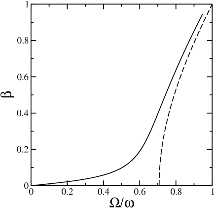
Figure 1: The upper branch of solution for the phase parameter $\beta$ of the hydrodynamic approach for a stationary vortex free BCS state in the rotating frame, as a function of the rotation frequency. Solid line: the trap anisotropy is $\epsilon=0.1$. Dashed line: $\epsilon=0$.

From the studies of the bosonic case Sinha it is known that the significantly deformed clouds can become dynamically unstable. We recall briefly the calculation procedure: one introduces initially arbitrarily small deviations $\delta\rho$ and $\delta S$ of the density and the phase from their stationary values; one then linearizes the hydrodynamic equations Eq.(12) and Eq.(13) to get

$$\frac{D\,\delta\rho}{Dt} = -\mathrm{div}\,\left(\rho\frac{\mathbf{grad}\,\delta S}{m}\right)$$ (16)

$$\frac{D\,\delta S}{Dt} = -\frac{\pi\hbar^{2}}{m}\,\delta\rho$$ (17)

where $D/Dt\equiv\partial_{t}+(\mathbf{v}-\mathbf{\Omega}\times\mathbf{r})\cdot\mathbf{grad}$ and where we used the fact that the Laplacian of $S(\mathbf{r})\propto xy$ vanishes. One then calculates the eigenmodes of the linearized equations, setting $\partial_{t}\rightarrow-i\nu$ where $\nu$ is the eigenfrequency of the mode. As an ansatz for $\delta\rho(\mathbf{r})$ and $\delta S(\mathbf{r})$, one takes polynomials of arbitrary total degree $n$ in the variables $x$ and $y$. One can indeed check that the subspace of polynomials of degree $\leq n$ is stable, since the stationary values $\rho$ and $S$ are quadratic functions of $x$ and $y$. This turns the linearized partial differential equations into a finite size linear system whose eigenvalues can be calculated numerically. Complex eigenfrequencies, when obtained, lead to a non-zero Lyapunov exponent $\lambda\equiv\mathrm{Im}\,\nu$, which reveals a dynamical instability when $\lambda>0$.

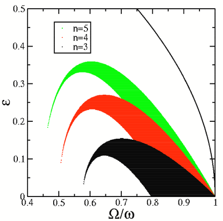
Figure 2: For the upper branch of solution for the phase parameter, in 2D: Dark areas: instability domain in the $\Omega-\epsilon$ plane for degrees $n$ equal to 3, 4 and 5 (crescents from bottom to top). There is no dynamical instability for $n\leq 2$. Solid line: border $\Omega^{2}=(1-\epsilon)\omega$ of the branch existence domain.

In figure 2 we plot the stability diagram of the upper branch stationary solution in the plane $(\Omega,\epsilon)$, for various total degrees $n$ of the polynomial ansatz. Each degree contributes to this diagram in the form of a crescent, touching the horizontal axis ($\epsilon=0$) with a broad basis on the right side and a very narrow tongue on the left side to_be_complete . For the low value $\epsilon=0.1$ considered in the numerical simulations of this paper, the Lyapunov exponents in the tongues are rather small, so that significant instability exponents are found only in the broad bases: for increasing $\Omega$, the first encountered significant instability corresponds to a degree $n=3$: for $\epsilon=0$, the corresponding minimal value of $\Omega/\omega$ is $(\frac{183+36\sqrt{30}}{599})^{1/2}=0.79667\ldots$ how_to_get_that . This is apparent in figure 3, where we plot the Lyapunov exponent as a function of $\Omega/\omega$ for various degrees $n$ and for $\epsilon=0.1$.

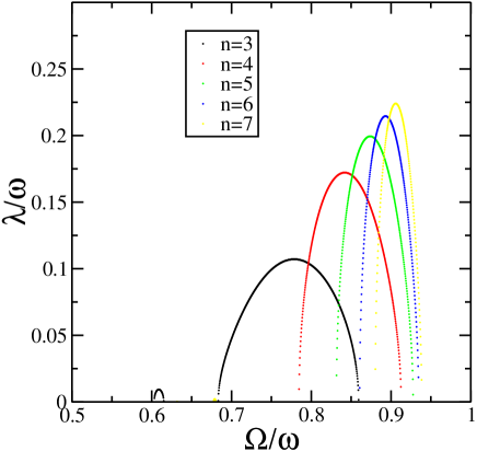
Figure 3: For the upper branch of solution for the phase parameter in 2D: Lyapunov exponent of the dynamic instability for degrees $n$ from 3 to 7, as a function of the rotation frequency. The trap anisotropy is $\epsilon=0.1$.

Extension to the unitary quantum gas in 3D: In practice, the experiments are mainly performed in 3D, so that we generalize the previous hydrodynamic calculation to a 3D case where the exact equation of state is known: the so-called unitary regime, where the 3D $s$-wave scattering length between opposite spin fermions is infinite. Because of the universality of the unitary quantum gas, the equation of state of the gas is indeed a power law

$$\mu_{0}[\rho]=A\rho^{\gamma}$$ (18)

where the exponent $\gamma=2/3$ and where the factor $A$ is proportional to $\hbar^{2}/m$, with a proportionality constant recently calculated with fixed node Monte Carlo methods Pandha ; Giorgini and measured in recent experiments by Grimm Grimm_eta and by Salomon MolecBEC .

For such a non-linear equation of state, one seems to have lost the underlying structure of the hydrodynamic equations allowing a quadratic ansatz for $\rho$ and $S$, and a polynomial ansatz for $\delta\rho$ and $\delta S$. Fortunately, this structure can be restored by using as a new variable $R(\mathbf{r},t)\equiv\rho^{\gamma}(\mathbf{r},t)$. One then gets effective hydrodynamic equations with a linear equation of state:

$$\partial_{t}R = -\gamma R\,\mathrm{div}\,\mathbf{v}-(\mathbf{v}-\mathbf{\Omega}(t)\times\mathbf{r})\cdot\mathbf{grad}\,R$$ (19)

$$-\partial_{t}S = \frac{1}{2}mv^{2}+U_{3D}(\mathbf{r})+A\,R(\mathbf{r})$$ (20)

$$-\mu-m(\mathbf{\Omega}(t)\times\mathbf{r})\cdot\mathbf{v},$$

where the 3D trapping potential is

$$U_{3D}(\mathbf{r})=\frac{1}{2}m\omega^{2}\left[(1-\epsilon)x^{2}+(1+\epsilon)y^{2}\right]+\frac{1}{2}m\omega_{z}^{2}z^{2}.$$ (21)

One then recycles the previous approach, with the usual quadratic ansatz for the steady state values of $R$ and $S$. In particular the same cubic equation for $\beta$ as in Eq.(15) is obtained. Linearizing the effective hydrodynamic equations around the steady state, one gets

$$\frac{D\,\delta R}{Dt} = -\gamma R\frac{\Delta_{\mathbf{r}}\delta S}{m}-\frac{1}{m}\,\mathbf{grad}\,\delta S\cdot\mathbf{grad}\,R$$ (22)

$$\frac{D\,\delta S}{Dt} = -A\,\delta R,$$ (23)

where we used the fact that $S$ has a vanishing Laplacian. This system of partial different equations can be solved by a polynomial ansatz for $\delta S$ and $\delta R$. This generalizes to the rotating case the ansatz of Minguzzi .

In figure 4 we have plotted the stability diagram of the upper branch stationary solution in the plane $(\Omega,\epsilon)$ for the 3D unitary quantum gas, for a trapping potential with $\omega_{z}=0.4\omega$. The 3D nature of the problem makes the structure of the instability domain more involved that in 2D. This also appears in figure 5, giving the Lyapunov exponents as a function of $\Omega$ for a fixed trap anisotropy in the $x-y$ plane, $\epsilon=0.022$. In the limit of a cigar shaped potential, $\omega_{z}\ll\omega$, the structure is on the contrary close to the 2D one, as some of the eigenmodes for $\delta R$ and $\delta S$ almost factorize in a function of $x,y$ and a function of $z$.

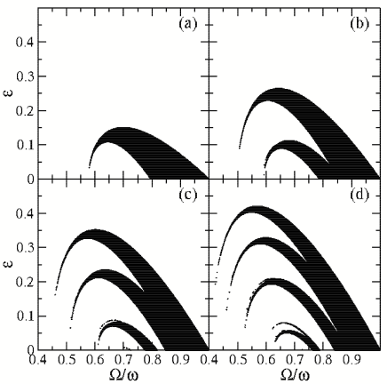
Figure 4: Case of the 3D unitary quantum gas with $\omega_{z}=0.4\omega$, for the upper branch of solution for the phase parameter: Dark areas: instability domain in the $\Omega-\epsilon$ plane for degrees (a) $n=3$, (b) $n=4$, (c) $n=5$ and (d) $n=6$. There is no dynamical instability for $n\leq 2$.

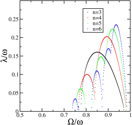
Figure 5: Case of the 3D unitary quantum gas with $\omega_{z}=0.4\omega$, for the upper branch of solution for the phase parameter: Maximal Lyapunov exponent of the dynamic instability for degrees $n$ from 3 to 6, as a function of the rotation frequency. The trap anisotropy is $\epsilon=0.022$.

III Numerical solution of the 2D time dependent BCS equations

We recall briefly the BCS equations for our two-component lattice model, in the case of equal populations of the two spin states. In the non-rotating case, the many-body ground state of the Hamiltonian is approximated variationally in the zero temperature BCS theory by a so-called quasiparticle vacuum Blaizot , that is the vacuum state of annihilation operators of elementary excitations, $b_{s,\sigma}$ (where $\sigma=\uparrow$ or $\downarrow$). By energy minimization, one finds that the $b_{s,\sigma}$ are such that

$$\psi_{\uparrow}(\mathbf{r}) = \sum_{s}\left[b_{s,\uparrow}u_{s}(\mathbf{r})-b_{s,\downarrow}^{\dagger}v_{s}^{*}(\mathbf{r})\right]$$ (24)

$$\psi_{\downarrow}(\mathbf{r}) = \sum_{s}\left[b_{s,\downarrow}u_{s}(\mathbf{r})+b_{s,\uparrow}^{\dagger}v_{s}^{*}(\mathbf{r})\right]$$ (25)

where the $u$’s and $v$’s are all the eigenvectors of the following Hermitian system with positive energies $E_{s}>0$:

$$E_{s}\,\left(\begin{tabular}[]{c}$u_{s}$\\ $v_{s}$\end{tabular}\right)=\left(\begin{tabular}[]{cc}$h_{0}$&$\Delta$\\ $\Delta^{*}$&$-h_{0}^{*}$\end{tabular}\right)\left(\begin{tabular}[]{c}$u_{s}$\\ $v_{s}$\end{tabular}\right)$$ (26)

and normalized so that

$$l^{2}\sum_{\mathbf{r}}\left[|u_{s}(\mathbf{r})|^{2}+|v_{s}(\mathbf{r})|^{2}\right]=1.$$ (27)

In the eigensystem, $\Delta$ is the position dependent gap parameter defined in Eq.(10) and the matrix $h_{0}$ represents on the lattice the single particle kinetic energy plus chemical potential plus harmonic potential energy terms. When the modal decompositions Eqs.(24,25) are inserted in Eq.(10), one gets

$$\Delta(\mathbf{r})=-g_{0}\sum_{s}u_{s}(\mathbf{r})v_{s}^{*}(\mathbf{r}).$$ (28)

The density profile of the gas is given by

$$\rho(\mathbf{r})=2\langle\psi_{\uparrow}^{\dagger}(\mathbf{r})\psi_{\uparrow}(\mathbf{r})\rangle=2\sum_{s}|v_{s}(\mathbf{r})|^{2}.$$ (29)

These equations actually belong to the zero temperature Hartree-Fock-Bogoliubov formalism for fermions and are derived in §7.4b of Blaizot . Note that we have omitted the Hartree-Fock mean field term mean_field .

To solve numerically the 2D self-consistent stationary BCS equations, we have used the following iterative algorithm: one starts with an initial guess for the position dependence of the gap parameter (we used the local density approximation, taking advantage of the fact that the equation of state Eq.(2) and the value of the gap Eq.(4) within BCS theory are known analytically in 2D), then one calculates the $u$’s and $v$’s by diagonalization of the Hermitian matrix in Eq.(26), one calculates the corresponding $\Delta(\mathbf{r})$ using Eq.(28), and one iterates until convergence.

Once the stationary BCS state is calculated, one moves to the solution of the 2D time dependent BCS equations, to calculate the dynamics in the rotating trap. What we call here time dependent BCS theory is the time-dependent Hartree-Fock-Bogoliubov formalism for fermions, in the form of a variational calculation with a time dependent quasiparticle vacuum $|\phi(t)\rangle$, as detailed in §9.5 of Blaizot . At time $t$, the modal expansions Eqs.(24,25) still hold for $\psi_{\uparrow}(\mathbf{r})$ and $\psi_{\downarrow}(\mathbf{r})$, except that the operators $b_{s,\sigma}$ (where $\sigma=\uparrow$ or $\downarrow$) and the mode functions are now time dependent. The variational state vector $|\phi(t)\rangle$ is the vacuum of all the operators $b_{s,\sigma}(t)$. The mode functions evolve according to

$$i\hbar\partial_{t}\,\left(\begin{tabular}[]{c}$u_{s}$\\ $v_{s}$\end{tabular}\right)=\left(\begin{tabular}[]{cc}$h_{0}$&$\Delta$\\ $\Delta^{*}$&$-h_{0}^{*}$\end{tabular}\right)\left(\begin{tabular}[]{c}$u_{s}$\\ $v_{s}$\end{tabular}\right)$$ (30)

where $h_{0}$ now includes the rotational term $-\Omega(t)L_{z}$ in addition to the kinetic energy, the chemical potential and the trapping potential. The gap function $\Delta$ is still given by Eq.(28) and is now time dependent as the mode functions are. Note that Eq.(30) corresponds to the first of the equations (9.63b) in §9.5 of Blaizot , up to a global complex conjugation. To be complete, we give the expression of the time dependent quasiparticle annihilation operators:

$$b_{s,\uparrow}(t) = l^{2}\sum_{\mathbf{r}}u_{s}^{*}(\mathbf{r},t)\psi_{\uparrow}(\mathbf{r})+v_{s}^{*}(\mathbf{r},t)\psi_{\downarrow}^{\dagger}(\mathbf{r})$$ (31)

$$b_{s,\downarrow}(t) = l^{2}\sum_{\mathbf{r}}u_{s}^{*}(\mathbf{r},t)\psi_{\downarrow}(\mathbf{r})-v_{s}^{*}(\mathbf{r},t)\psi_{\uparrow}^{\dagger}(\mathbf{r}).$$ (32)

We also recall that this time-dependent formalism contains not only pair-breaking excitations, but also implicitly collective modes of the gas, as can be shown by a linearization of these equations around a steady-state solution, see §10.2 in Blaizot , and as also shown by the fact that hydrodynamic equations may be derived from them as done in the Appendix A. The numerical simulations to come therefore include excitations of these collective modes, when the numerical solution deviates from a stationary state.

We have integrated numerically Eq.(30). The usual FFT split technique, which exactly preserves the orthonormal nature of the $u$’s and $v$’s, is actually not satisfactory because it assumes that the gap function remains constant in time during one time step, which breaks the self-consistency of the equations and leads to a violation of the conservation of the mean number of particles. We therefore used an improved splitting method detailed in the appendix B.

In all the simulations that we present in this paper, the trap anisotropy was $\epsilon=0.1$, the chemical potential of the initial state of the gas was fixed to $\mu=8\hbar\omega$; setting $\mu=\hbar^{2}k_{F}^{2}/2m$, the 2D scattering length was fixed to the value $a_{\rm 2D}=(\hbar/m\omega)^{1/2}\equiv a_{\rm ho}$ such that $k_{F}a_{\rm 2D}=4$; the rotation frequency was turned on with the following law

$$\Omega(t)=\Omega\,\sin^{2}\left(\frac{\pi t}{2\tau}\right)\ \ \ \ \mbox{for}\ \ 0\leq t\leq\tau$$ (33)

with a ramping time $\tau=160\omega^{-1}$ much larger than the oscillation period of the atoms in the trap. For $t>\tau$, the rotation frequency remains equal to $\Omega$. The presence of vortices is detected by calculating the winding number of the phase of the gap parameter around each plaquette of the grid. We also calculated the total angular momentum of the gas. In all the simulations, we evolved the system for a total time of $1000\,\omega^{-1}$.

Simulations on a small $32\times 32$ grid: For such a grid size, the calculation time remains reasonable so that we varied the final rotation frequency in steps of $0.1\omega$. For final rotation frequencies $\Omega\leq 0.3\omega$, no vortices are found to enter the cloud and the cloud remains round.

For $\Omega=0.4\omega$, the cloud remains round but a corrugation of the surface of the cloud is observed to appear at time $t\simeq 240\omega^{-1}$; the amplitude of the corrugation increases and two diametrically opposite vortices enter the cloud gently at $t\simeq 400\omega^{-1}$ and, after a time interval of $\sim 100\omega^{-1}$, settle in a stationary pair of vortices close to the trap center. At $t\simeq 700\omega^{-1}$, a second pair of vortices starts entering with the same mechanism; it then interacts with the first pair. The 4 vortices arrange in a stationary square at $t\simeq 850\omega^{-1}$. For $\Omega=0.5\omega$, the situation is similar: one vortex pair enters, then a second one, then a triplet of vortices starts entering at $t\simeq 490\omega^{-1}$; eventually, at $t>610\omega^{-1}$ the seven vortices arrange in a stationary regular pattern, consisting of an hexagon plus a vortex in the center. Selected images of the movie of the simulation for $\Omega=0.5\omega$ are shown in figure 6. For $\Omega=0.6\omega$, the scenario is slightly different. The corrugation of the surface is stronger, and a rectangular pattern of 4 vortices enter at time $t\simeq 220\omega^{-1}$, shortly followed at $t\simeq 250\omega^{-1}$ by a second rectangular pattern of 4 vortices. After an interaction period, 6 vortices align in the cloud in two parallel rows whereas two vortices are pushed away. Then a third rectangle of vortices enter. At later times, several extra vortices join the group; from $t\simeq 500\omega^{-1}$ til the end of the simulation, 12 vortices are present in the cloud, forming an almost stationary and regular pattern. Clearly, in these scenarios, no global turbulence of the cloud is involved, since the first entering vortices are arranged in a preformed pattern obeying the parity symmetry of the Hamiltonian.

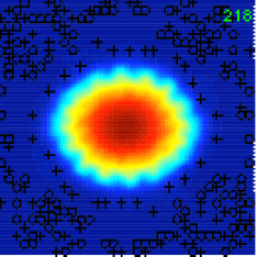
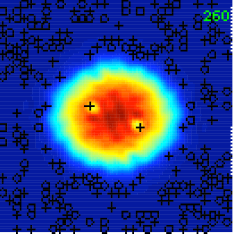
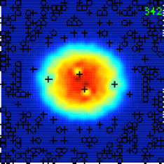
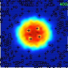
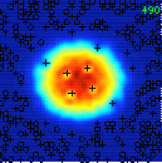
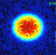
Figure 6: For the numerical simulation of the 2D time dependent BCS equations on a $32\times 32$ grid, density plots of the density of the trapped gas at selected times (in units of $\omega^{-1}$), for a final rotation frequency $\Omega=0.5\omega$. The trap anisotropy was $\epsilon=0.1$ and the 2D scattering length $a_{2D}=\sqrt{\hbar/m\omega}$, and $\mu=8\hbar\omega$ in the initial state. The full spatial width of the simulation grid is shown in the figure. Crosses: positive charge vortices. Circles: negative charge vortices. From top to bottom and from left to right: $t=218\omega^{-1}$: a corrugation of the surface appears; $t=260\omega^{-1}$: a vortex pair enters; $t=342\omega^{-1}$: a second vortex pair enters; $t=400\omega^{-1}$: the vortices arrange on a square; $t=490\omega^{-1}$: a triplet of vortices starts entering; $t=610\omega^{-1}$: a stationary 7-vortex pattern.

For $\Omega=0.7\omega$ and $\Omega=0.8\omega$ the dynamics is very different from the previous one. The shape of the cloud strongly elongates and deforms. Then strong turbulence sets in, at $t\simeq 160\omega^{-1}$ for $\Omega=0.7\omega$ ($t\simeq 135\omega^{-1}$ for $\Omega=0.8\omega$), while the cloud anisotropy reduces, the density profile becomes irregular, not only close the cloud boundary but also in the cloud center; one observes a quick entrance of disordered vortices in the cloud at time $t\simeq 190\omega^{-1}$ for $\Omega=0.7\omega$ ($t\simeq 150\omega^{-1}$ for $\Omega=0.8\omega$); several anti-vortices reach the borders of the cloud for $\Omega=0.7\omega$ and even reach high density regions for $\Omega=0.8\omega$. After some evolution time, the density profile recovers a smooth and elliptic shape, the anti-vortices are expelled from the cloud and the vortex positions slowly relax to form a 17 (or 25 for $\Omega=0.8\omega$) vortex ‘lattice’ at times $\sim 500\omega^{-1}$, that remains essentially stationary til the end of the simulation.

In conclusion, two distinct scenarios of vortex lattice formation are observed in the $32\times 32$ simulations. For the lower rotation frequencies, a gentle entry of an ordered pattern of vortices is observed. For the higher rotation frequencies, turbulence sets in and leads to the abrupt and disordered entrance of vortices and even anti-vortices, the regular and stationary vortex ‘lattice’ forming after some evolution time. Another difference between the two scenarios is the temporal behavior of the density profile at the location of the vortex cores: whereas a dip in the density is visible from the start when a vortex enters the cloud with the gentle scenario, such a dip at the vortex location forms only after some relaxation time in the turbulent scenario.

The physical origin of the turbulent scenario is expected to be the dynamic instability of the mode of degree $n=3$ discussed in section II, and the obtained movies qualitatively agree with that. More quantitatively: for $\epsilon=0.1$ a significant Lyapunov exponent is obtained for $\Omega>0.68\omega$; this is compatible with the fact that the numerical simulation observes turbulence for $\Omega\geq 0.7\omega$ only.

What is the physical origin of the gentle scenario ? The observed corrugation at the surface suggests that it is driven by the instability of some surface mode localized at the surface of the cloud, which is reminiscent of the Landau mechanism. As a test of this idea, we have performed a numerical calculation of the stationary BCS state in a rotating frame, by the above mentioned iterative scheme: as shown in figure 7 giving the angular momentum of the stationary BCS solution as a function of the rotation frequency, for $\epsilon=0.1$, the branch with no vortex is followed up to $\Omega=0.3\omega$; for larger values of $\Omega$, the algorithm jumps to a configuration with vortices. This suggests that the vortex free BCS state is indeed not a local minimum of energy for $\Omega>0.3\omega$. What is then puzzling at this stage is that a harmonic stirrer can excite only the quadrupolar modes, whereas the negative energy surface mode initiating the Landau mechanism is expected to have a higher angular momentum Dalfovo . A possible solution to this paradox was obtained by running the time dependent simulation with $\epsilon=0$, for $\Omega=0.5\omega$: in this case, the harmonic trap, being isotropic, can not stir the gas and the stirring is due only to the fixed periodic boundary conditions in the rotating frame; still, vortices were found to enter the cloud. This shows that the quantization box in our $32\times 32$ simulations is small enough to activate the Landau mechanism.

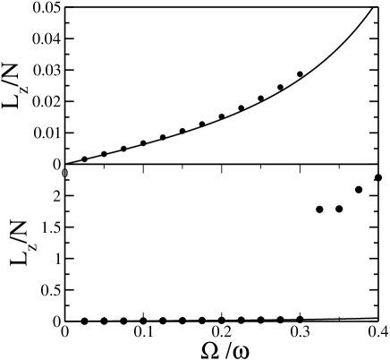
Figure 7: In a steady state solution of the 2D BCS theory, on a $32\times 32$ grid, angular momentum per particle in the gas, in units of $\hbar$, as a function of the rotation frequency, for $\epsilon=0.1$ and $\mu=8\hbar\omega$, $a_{2D}=(\hbar/m\omega)^{1/2}$. Black disks: numerical result from an iterative algorithm (no vortex at the left part of the jump, vortices present at the right part of the jump). Solid line: hydrodynamic prediction (no vortex). The upper graph corresponds to the same data as the lower graph, but for a different scale of the vertical axis: it shows the good agreement of the hydrodynamic prediction with the full numerics. In the numerics, the total number of particles is $\sim 72$ on the left part of the jump, and reaches $\sim 80$ on the most right data point; the rotation frequency is increased step by step from 0 to 0.4$\omega$, the converged state for a given $\Omega$ being taken as an initial guess in the iterative algorithm for the successive value of $\Omega$.

Simulations on larger grids: To get rid of the previously mentioned finite quantization box effects, we performed simulations on larger grids, $48\times 48$ and $64\times 64$. For the $48\times 48$ grids, we investigated the rotation frequencies from $0.4\omega$ to $0.8\omega$ in steps of $0.1\omega$. No vortex is found to enter the cloud for $\Omega\leq 0.5\omega$. For $\Omega=0.6\omega$, vortices enter according to the gentle scenario; the first vortices (in the form of a pair) enter however at a considerable later time, $t\simeq 400\omega^{-1}$, than with the $32\times 32$ grid simulation. For $\Omega\geq 0.7\omega$ the vortices enter according to the turbulent scenario. The turbulent scenario on the $48\times 48$ grid is similar to the one observed on the $32\times 32$ grid, except for temporal shifts: e.g.  on the $48\times 48$ grid, the turbulent period starts $\simeq 240\omega^{-1}$ later for $\Omega=0.7\omega$ and $\simeq 65\omega^{-1}$ later for $\Omega=0.8\omega$.

For the $64\times 64$ grids, the CPU time for a single realization exceeds one month on a bi-processor AMD Opteron workstation, so that we have considered only two values of the rotation frequency. For $\Omega=0.6\omega$, no entry of vortices is observed. This confirms that the observation of the gentle scenario, at least up to the maximal evolution time (1000$\omega^{-1}$) considered here, is an artifact of the quantization box. For $\Omega=0.8\omega$, vortices enter according to the turbulent scenario. The timing is now quantitatively the same at the $48\times 48$ simulation: in both simulations, the vortices enter the cloud at $t\simeq 205\omega^{-1}$ and crystallize in a quasi stationary pattern at times $\sim 500-550\omega^{-1}$. Selected images of the movie of the $64\times 64$ simulation for $\Omega=0.8\omega$ are shown in figure 8.

To allow for a quantitative comparison between the simulations for the three grid sizes, we have plotted in figure 9 the total angular momentum of the gas as a function of time, for (a) $\Omega=0.6\omega$ and (b) $\Omega=0.8\omega$. We have also given the (vortex free) hydrodynamic prediction; remarkably, this shows that the simulations give results close to the hydrodynamic one as long as no vortex enters the cloud, see in particular the $64\times 64$ results for $\Omega=0.6\omega$. To briefly address the experimental observability of the vortex pattern, we also show in figure 10 a cut of the particle density (directly measurable in an experiment) and of the gap parameter (not directly accessible experimentally) for the $64\times 64$ simulation with $\Omega=0.8\omega$ at a time when the vortex lattice is crystallized, this in parallel to an isocontour of the magnitude of the gap parameter: vortices embedded in high density regions result in dips in the density profile, with a contrast on the order here of 30%.

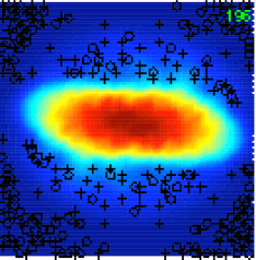
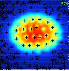
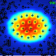
Figure 8: For the numerical simulation of the 2D time dependent BCS equations on a $64\times 64$ grid, density plots of the density of the trapped gas at selected times (in units of $\omega^{-1}$), for a final rotation frequency $\Omega=0.8\omega$. The trap anisotropy was $\epsilon=0.1$ and the 2D scattering length $a_{2D}=\sqrt{\hbar/m\omega}$, and $\mu=8\hbar\omega$ in the initial state. The spatial width of the simulation is truncated in the figure to have approximately the same width as in Fig.6. Crosses: positive charge vortices. Circles: negative charge vortices. From top to bottom and from left to right: $t=196\omega^{-1}$: a turbulent, elongated cloud is formed; $t=212\omega^{-1}$: the cloud is round again, and includes a disordered mixture of vortices and anti-vortices; $t=574\omega^{-1}$: the vortices crystallize in a quasi-stationary pattern; $t=998\omega^{-1}$: slow and small shifts of some vortex positions have taken place with respect to the previous density plot.

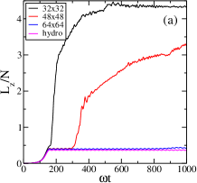
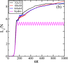
Figure 9: Angular momentum per particle in the gas, in units of $\hbar$, as a function of time, for a final rotation frequency (a) $\Omega=0.6\omega$ and (b) $\Omega=0.8\omega$. Curves (from top to bottom in (a)): numerical simulations of the 2D time dependent BCS equations for the grids $32\times 32$, $48\times 48$ and $64\times 64$, and for the time dependent superfluid hydrodynamic theory of section II.

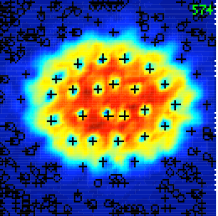
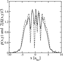
Figure 10: At time $t=574\omega^{-1}$ of the $64\times 64$ numerical simulation for $\Omega=0.8\omega$. Left panel: isocontours of the modulus of the gap parameter, showing the presence of a vortex lattice; the $x$ and $y$ coordinates run from $-10a_{\rm ho}$ to $+10a_{\rm ho}$ in the simulation but this left panel figure is truncated to a position interval approximately $-7a_{\rm ho}$ to $+7a_{\rm ho}$. Right panel: on the line $y=-0.627a_{\rm ho}$, $x$ dependence of the density $\rho$ (solid line, in units of $a_{\rm ho}^{-2}$) and of the modulus of the gap parameter (dashed line, in units of $\hbar\omega$). The gap parameter was multiplied by 2/3 for clarity. A Fourier interpolation technique was used in the right panel to map the 64$\times$64 simulation grid onto a 128$\times$128 grid.

IV Conclusion

We have investigated a relevant problem for the present experiments on two-spin component interacting Fermi gases, the possibility to form a vortex lattice by slow ramping of the rotation frequency of the harmonic trap containing the particles. The observation of such a vortex lattice in steady state would be a very convincing evidence of superfluidity vort_ketterle .

For a 2D model based on the BCS theory, and for the 3D unitary quantum gas, we predict analytically, with the superfluid hydrodynamic equations, that the gas experiences a dynamic instability when the final rotation frequency is above some minimal value $\Omega_{u}$ that we have calculated. This dynamic instability is very similar to the one discovered for a rotating Bose-Einstein condensate of bosonic atoms, where it was shown to lead to the vortex lattice formation.

To see if this dynamic instability leads to the formation of vortices also in the case of the Fermi gases, we have solved numerically the full 2D time-dependent BCS equations, for a trap anisotropy $\epsilon=0.1$. For a final rotation frequency $\Omega$ above the predicted $\Omega_{u}$, we see turbulence and the subsequent fast entry of vortices. We conclude that the dynamic instability can indeed result in a vortex lattice formation. The apparent irreversibility and energy dissipation that this seems to imply may be surprising at first sight, since the equations of motion that we integrated are purely conservative. The clue is probably the same as in the bosonic counterpart of these simulations Sinatra : the spatial noise produced in the turbulent phase populates many eigenmodes (including collective modes) of the system, and the subsequent non-linear evolution leads to effective thermalization of the modes.

For $\Omega<\Omega_{u}$ but for $\Omega$ larger than what we estimated to be the Landau rotation frequency (above which the vortex free superfluid is no longer a local minimum of energy in the rotating frame), we also see the formation of a vortex lattice in the simulations on the small $32\times 32$ grids, but with a gentle mechanism not involving turbulence and leading to the entrance of a pre-formed regular vortex pattern from the surface of the cloud. But we also performed simulations on larger grids: on a $64\times 64$ grid, the gentle mechanism disappears; it is therefore an artifact of the periodic boundary conditions that rotate in the lab frame and provide an artificial stirring effect. In a real experiment, however, we expect such a gentle mechanism to occur for a gas initially at finite temperature, when the normal component of the gas is set into rotation by the stirrer.

Appendix A Simple derivation of the hydrodynamic equations from BCS theory

We show here that the time dependent hydrodynamic equations Eq.(12) and Eq.(13) can be formally derived for a vortex free gas from the time dependent BCS equations by using the lowest order semi-classical approximation and an adiabatic approximation for the resulting time dependent equations. As in the remaining part of the paper, we consider here the regime where the chemical potential is positive and larger than the binding energy $E_{0}$.

The general validity condition of a semi-classical approximation is that the coherence length of the gas should be much smaller than the typical length scales of variation of the applied potentials. Two coherence lengths appear for a zero temperature BCS Fermi gas: the inverse Fermi wave-vector, $k_{F}^{-1}$, associated to the correlation function $\langle\psi^{\dagger}_{\uparrow}(\mathbf{r})\psi_{\uparrow}(\mathbf{r^{\prime}})\rangle$, and the pair size, $l_{\rm BCS}\sim\hbar^{2}k_{F}/m|\Delta|$, associated to the correlation function $\langle\psi_{\uparrow}(\mathbf{r})\psi_{\downarrow}(\mathbf{r^{\prime}})\rangle$. A first typical length scale of variation of the matrix elements in Eq.(30) comes from the position dependence of $|\Delta|$: in the absence of rotation, we assume that this is the Thomas-Fermi radius $R_{\rm TF}$ of the gas, defined as $\hbar^{2}k_{F}^{2}/2m=m\omega^{2}R_{\rm TF}^{2}/2$. This assumes that the scale of variation of the modulus of the gap is the same as the one of the density; the adiabatic approximation to come will result in a $|\Delta|$ related to the density by Eq.(4), which justifies the assumption. Necessary validity conditions of a semi-classical approximation are then:

$$k_{F}^{-1},l_{\rm BCS}\ll R_{\rm TF}.$$ (34)

In the BCS regime regime, $k_{F}^{-1}<l_{\rm BCS}$; for an isotropic harmonic trap, one then finds that the condition Eq.(34) is equivalent to

$$|\Delta|\gg\hbar\omega,$$ (35)

where $\omega$ is the atomic oscillation frequency. The presence of vortices introduces an extra length scale in the variation of $|\Delta|$, on the order of $l_{\rm BCS}$, which invalidates the semi-classical approximation.

In the rotating case, however, this is not the whole story, as the phase of $\Delta$ can also become position dependent. As we shall see, the phase of $\Delta$ in this paper may vary as $m\omega xy/\hbar$: when this quantity varies by $\sim 2\pi$, $\Delta$ changes completely; this introduces a length scale $\sim 2\pi\hbar/(m\omega R_{\rm TF})\sim 1/k_{F}$, making a semi-classical approximation hopeless. We eliminate this problem by performing a gauge transform of the $u$’s and $v$’s:

$$\tilde{u}_{s}(\mathbf{r},t) \equiv u_{s}(\mathbf{r},t)e^{-iS(\mathbf{r},t)/\hbar}$$ (36)

$$\tilde{v}_{s}(\mathbf{r},t) \equiv v_{s}(\mathbf{r},t)e^{+iS(\mathbf{r},t)/\hbar}$$ (37)

where the phase is defined in Eq.(10). The time dependent BCS equations are modified as follows:

$$i\hbar\partial_{t}\,\left(\begin{tabular}[]{c}$\tilde{u}_{s}$\\ $\tilde{v}_{s}$\end{tabular}\right)=\left(\begin{tabular}[]{cc}$\tilde{h}_{0}$&$|\Delta|$\\ $|\Delta|$&$-\tilde{h}_{0}^{*}$\end{tabular}\right)\left(\begin{tabular}[]{c}$\tilde{u}_{s}$\\ $\tilde{v}_{s}$\end{tabular}\right)\equiv\hat{L}\left(\begin{tabular}[]{c}$\tilde{u}_{s}$\\ $\tilde{v}_{s}$\end{tabular}\right)$$ (38)

where the gauge transformed Hamiltonian is

$$\tilde{h}_{0}=e^{-iS/\hbar}h_{0}e^{+iS/\hbar}+\partial_{t}S.$$ (39)

Let us review relevant observables in the gauge transformed representation. First the gap equation is modified as

$$|\Delta|=-g_{0}\sum_{s}\tilde{u}_{s}\tilde{v}_{s}^{*}.$$ (40)

Then the mean total density reads

$$\rho=2\sum_{s}\tilde{v}_{s}\tilde{v}_{s}^{*}.$$ (41)

Last, we introduce the total matter current $\mathbf{j}(\mathbf{r},t)$, that obeys by definition

$$\partial_{t}\rho+\mathrm{div}\,\mathbf{j}=0.$$ (42)

In the rotating frame, in a many-body state invariant by exchange of the spin states $\uparrow$ and $\downarrow$, it is very generally given by

$$\mathbf{j}=\frac{\hbar}{im}\left(\langle\psi_{\uparrow}^{\dagger}\mathbf{grad}\,\psi_{\uparrow}\rangle-\mbox{c.c.}\right)-\rho\,\mathbf{\Omega}\times\mathbf{r}.$$ (43)

Within BCS theory, this gives

$$\mathbf{j}=\rho\,(\mathbf{v}-\mathbf{\Omega}\times\mathbf{r})+\frac{i\hbar}{m}\sum_{s}\left[\tilde{v}_{s}^{*}\,\mathbf{grad}\,\tilde{v}_{s}-\tilde{v}_{s}\,\mathbf{grad}\,\tilde{v}_{s}^{*}\right],$$ (44)

where the velocity field $\mathbf{v}$ is defined as $\mathbf{grad}\,S/m$. Note that the continuity equation Eq.(42) remains true for the BCS theory Blaizot .

To calculate the two key quantities Eq.(41) and Eq.(44), it is sufficient to know the following one-body density operator for a fictitious particle of spin 1/2,

$$\sigma=\left(\begin{tabular}[]{cc}$\sigma_{\uparrow\uparrow}$&$\sigma_{\uparrow\downarrow}$\\ $\sigma{\downarrow\uparrow}$&$\sigma_{\downarrow\downarrow}$\end{tabular}\right)\equiv\sum_{s}\left(\begin{tabular}[]{cc}$|\tilde{u}_{s}\rangle\langle\tilde{u}_{s}|$&$|\tilde{u}_{s}\rangle\langle\tilde{v}_{s}|$\\ $|\tilde{v}_{s}\rangle\langle\tilde{u}_{s}|$&$|\tilde{v}_{s}\rangle\langle\tilde{v}_{s}|$\end{tabular}\right).$$ (45)

To prepare for the semi-classical approximation we introduce the Wigner representation of $\sigma$ Wigner :

$$W(\mathbf{r},\mathbf{p},t)=\mathrm{Wigner}\{\sigma\}\equiv\int\frac{d^{d}\mathbf{x}}{(2\pi\hbar)^{d}}\langle\mathbf{r}-\mathbf{x}/2|\sigma|\mathbf{r}+\mathbf{x}/2\rangle e^{i\mathbf{p}\cdot\mathbf{x}/\hbar}$$ (46)

where $d$ is the dimension of space. The key observables have then the exact expressions:

$$\rho(\mathbf{r},t) = 2\int d^{d}\mathbf{p}\,W_{\downarrow\downarrow}(\mathbf{r},\mathbf{p},t)$$ (47)

$$|\Delta|(\mathbf{r},t) = -g_{0}\int d^{d}\mathbf{p}\,W_{\uparrow\downarrow}(\mathbf{r},\mathbf{p},t)$$ (48)

$$\mathbf{j}(\mathbf{r},t) = \rho\,(\mathbf{v}-\mathbf{\Omega}\times\mathbf{r})$$ (49)

$$-\frac{2}{m}\int d^{d}\mathbf{p}\,\mathbf{p}\,W_{\downarrow\downarrow}(\mathbf{r},\mathbf{p},t).$$

The semi-classical expansion then consists e.g. in

$$\mathrm{Wigner}\{V(\hat{\mathbf{r}})\sigma\}=[V(\mathbf{r})+\frac{i\hbar}{2}\partial_{\mathbf{r}}V\cdot\partial_{\mathbf{p}}+\ldots]W(\mathbf{r},\mathbf{p},t).$$ (50)

The successive terms we called zeroth order, first order, etc, in the semi-classical approximation.

We write the equations of motion Eq.(38) up to zeroth order in the semi-classical approximation:

$$i\hbar\partial_{t}W(\mathbf{r},\mathbf{p},t)|^{(0)}=\left[L_{0}(\mathbf{r},\mathbf{p},t),W(\mathbf{r},\mathbf{p},t)\right]$$ (51)

where the matrix $L_{0}$ is equal to

$$L_{0}(\mathbf{r},\mathbf{p},t)=\left(\begin{tabular}[]{cc}$\frac{p^{2}}{2m}-\mu_{\rm eff}(\mathbf{r},t)$&$|\Delta|(\mathbf{r},t)$\\ $|\Delta|(\mathbf{r},t)$&$-\frac{p^{2}}{2m}+\mu_{\rm eff}(\mathbf{r},t)$\end{tabular}\right).$$ (52)

We have introduced the position and time dependent function,

$$\mu_{\rm eff}(\mathbf{r},t)\equiv\mu-U(\mathbf{r},t)-\frac{1}{2}mv^{2}+m\mathbf{v}\cdot(\mathbf{\Omega}\times\mathbf{r})-\partial_{t}S(\mathbf{r},t),$$ (53)

that may be called effective chemical potential for reasons that will become clear later.

At time $t=0$, the gas is at zero temperature. By introducing the spectral decomposition of $\hat{L}(t=0)$ one can then check that

$$\sigma(t=0)=\theta[\hat{L}(t=0)]$$ (54)

where $\theta(x)$ is the Heaviside function. Since $L_{0}(t=0)$ is the classical limit of the operator $\hat{L}(t=0)$, the leading order semi-classical approximation for the corresponding Wigner function is, in a standard way, given by

$$W(\mathbf{r},\mathbf{p},t=0)\simeq\frac{1}{(2\pi\hbar)^{d}}\,\theta[L_{0}(\mathbf{r},\mathbf{p},t=0)]$$ (55)

that is each two by two matrix $W$ is proportional to a pure state $|\psi\rangle\langle\psi|$ with

$$|\psi(\mathbf{r},\mathbf{p},t=0)\rangle=\left(\begin{tabular}[]{c}$U_{0}(\mathbf{r},\mathbf{p})$\\ $V_{0}(\mathbf{r},\mathbf{p})$\end{tabular}\right)$$ (56)

where $(U_{0},V_{0})$ is the eigenvector of $L_{0}(\mathbf{r},\mathbf{p},t=0)$ of positive energy and normalized to unity. At time $t$, according to the zeroth order evolution Eq.(51), each two by two matrix $W$ remains a pure state, with components $U$ and $V$ solving

$$i\hbar\partial_{t}\left(\begin{tabular}[]{c}$U(\mathbf{r},\mathbf{p},t)$\\ $V(\mathbf{r},\mathbf{p},t)$\end{tabular}\right)=L_{0}(\mathbf{r},\mathbf{p},t)\left(\begin{tabular}[]{c}$U(\mathbf{r},\mathbf{p},t)$\\ $V(\mathbf{r},\mathbf{p},t)$\end{tabular}\right)$$ (57)

We then introduce the so-called adiabatic approximation: the vector $(U,V)$, being initially an eigenstate of $L_{0}(\mathbf{r},\mathbf{p},t=0)$, will be an instantaneous eigenvector of $L_{0}(\mathbf{r},\mathbf{p},t)$ at all later times $t$. This approximation holds under the adiabaticity condition adiab , detailed below, requiring that the energy difference between the two eigenvalues of $L_{0}(\mathbf{r},\mathbf{p},t)$ (divided by $\hbar$) be large enough. As this energy difference can be as small as the gap parameter, this will impose a minimal value to the gap, as we shall discuss later. In this adiabatic approximation, one can take

$$W(\mathbf{r},\mathbf{p},t)=\frac{1}{(2\pi\hbar)^{d}}\,\theta[L_{0}(\mathbf{r},\mathbf{p},t)]=\frac{1}{(2\pi\hbar)^{d}}\,|+\rangle\langle+|$$ (58)

where $|+(\mathbf{r},\mathbf{p},t)\rangle$, of real components $(U_{\rm inst},V_{\rm inst})$, is the instantaneous eigenvector with positive eigenvalue of the matrix $L_{0}$ defined in Eq.(52). Its components are simply the amplitudes on the plane wave $\exp(i\mathrm{p}\cdot\mathrm{r}/\hbar)$ of the BCS mode functions of a spatially uniform BCS gas of chemical potential $\mu_{\rm eff}$ and of gap parameter $|\Delta(\mathbf{r},t)|$. Using Eq.(47) and Eq.(48) with the approximate Wigner distribution Eq.(58), one further finds that this fictitious spatially uniform BCS gas is at equilibrium at zero temperature so that the expressions Eq.(2) and Eq.(4) may be used. In particular, Eq.(2) gives

$$\mu_{\rm eff}(\mathbf{r},t)=\mu_{0}[\rho(\mathbf{r},t)]$$ (59)

which leads, together with Eq.(53), to one of the time dependent hydrodynamic equations, the Euler-type one Eq.(13). Also, $U_{\rm inst}$ and $V_{\rm inst}$ are even functions of $\mathbf{p}$, so that the integral in the right hand side of Eq.(49) vanishes and Eq.(42) reduces to the hydrodynamic continuity equation Eq.(12). Under the adiabatic approximation, the superfluid hydrodynamic equations are thus derived.

We now discuss the validity of the adiabatic approximation. Without this approximation, the two by two matrix $W$ has non-zero off-diagonal matrix elements $\langle+|W|-\rangle$ where $|-\rangle$ is the instantaneous eigenvector of Eq.(52) with a negative eigenvalue, that can be written $(V_{\rm inst},-U_{\rm inst})$. Writing from Eq.(51) the equation of motion for $\langle+|W|-\rangle$, one indeed finds a coupling to the diagonal element $\langle+|W|+\rangle$ due to the non infinite ramping time of the rotation. This coupling can be calculated using the off-diagonal Hellman-Feynman theorem for real eigenvectors, and corresponds to a Rabi frequency

$$\frac{1}{2}\nu_{\rm time}\equiv-\langle-|\partial_{t}|+\rangle=-\frac{1}{\epsilon_{+}-\epsilon_{-}}\langle-|\left(\partial_{t}L_{0}\right)|+\rangle$$ (60)

where $\epsilon_{\pm}$ is the eigenenergy of $|\pm\rangle$ for the matrix $L_{0}$:

$$\epsilon_{\pm}=\pm\left[\left(p^{2}/(2m)-\mu_{\rm eff}\right)^{2}+|\Delta|^{2}\right]^{1/2}.$$ (61)

But this is not the whole story, as we have neglected the so-called motional couplings, that can also destroy adiabaticity. These motional couplings are due to the fact that $|+\rangle$ and $|-\rangle$ depends on $\mathbf{r},\mathbf{p}$ and that terms involving $\partial_{\mathbf{p}}W$ and $\partial_{\mathbf{r}}W$ will appear in the equation for $W$ beyond the zeroth-order semi-classical approximation. Such non-adiabatic effects are well known for the motion of a spin $1/2$ particle in a static but spatially inhomogeneous magnetic field. In our problem, the first order term of the semi-classical expansion is actually simple to write:

$$\partial_{t}W|^{(1)}=\frac{1}{2}\left[\partial_{\mathbf{r}}L\cdot\partial_{\mathbf{p}}W-\partial_{\mathbf{p}}L\cdot\partial_{\mathbf{r}}W+\mbox{h.c.}\right].$$ (62)

The matrix $L$ corresponds to the classical limit of $\hat{L}(t)$:

$$L(\mathbf{r},\mathbf{p},t)=L_{0}(\mathbf{r},\mathbf{p},t)+\mathbf{p}\cdot\left(\mathbf{v}-\mathbf{\Omega}\times\mathbf{r}\right)\,\mbox{I},$$ (63)

where I is the $2\times 2$ identity matrix. In the resulting equation of evolution of $\langle+|W|-\rangle$, taking $\langle+|W|+\rangle=1/(2\pi\hbar)^{d}$ and $\langle-|W|-\rangle=0$, a motional Rabi coupling to $\langle+|W|+\rangle$ now appears:

$$\frac{1}{2}\nu_{\rm motion}\equiv -\partial_{\mathbf{p}}\left[\mathbf{p}\cdot(\mathbf{v}-\mathbf{\Omega}\times\mathbf{r})\right]\cdot\langle-|\partial_{\mathbf{r}}|+\rangle$$ (64)

$$+\partial_{\mathbf{r}}\left[\mathbf{p}\cdot(\mathbf{v}-\mathbf{\Omega}\times\mathbf{r})\right]\cdot\langle-|\partial_{\mathbf{p}}|+\rangle.$$

Expressions similar to the one for $\langle-|\partial_{t}|+\rangle$ can be derived with the off-diagonal Hellman-Feynman theorem.

We now calculate the total Rabi frequency $\nu_{\rm tot}\equiv\nu_{\rm time}+\nu_{\rm motion}$ at the local Fermi surface, that is for a value of the momentum such that $p^{2}/2m=\mu_{\rm eff}(\mathbf{r},t)$. This is indeed at the Fermi surface that we expect the adiabaticity condition to be most stringent, as the energy difference $\epsilon_{+}-\epsilon_{-}$ takes there its minimal value, equal to twice the gap $|\Delta(\mathbf{r},t)|$. Then $U_{\rm inst}=V_{\rm inst}=1/\sqrt{2}$ and the expressions resulting from the Hellman-Feynman theorem are very simple:

$$\langle-|\partial_{\lambda}|+\rangle=-\frac{\partial_{\lambda}(\mu_{\rm eff}-p^{2}/2m)}{2|\Delta|},$$ (65)

where $\lambda$ stands for $t$ or for an arbitrary component of the vectors $\mathbf{r}$ or $\mathbf{p}$. We then get the condition for adiabaticity:

$$\frac{|\nu_{\rm tot}|}{2}=\frac{1}{2|\Delta|}\left|\frac{D\mu_{\rm eff}}{Dt}+\left(\frac{\mathbf{p}\cdot\partial_{\mathbf{r}}}{m}\right)^{2}S\right|\ll 2|\Delta|/\hbar,$$ (66)

where $D/Dt=\partial_{t}+\left(\mathbf{v}-\mathbf{\Omega}\times\mathbf{r}\right)\cdot\partial_{\mathbf{r}}$.

A fully explicit expression for $\nu_{\rm tot}$ can be obtained using the hydrodynamic equations and taking the limit of a very long ramping time of the rotation, as is the case in our simulations, so that the hydrodynamic variables are close to a steady state and $S\simeq m\omega\beta(t)xy$. Using Eq.(59) and the continuity equation Eq.(12), one gets $D\mu_{\rm eff}/Dt=-\rho\mu_{0}^{\prime}[\rho]\mathrm{div}\,\mathbf{v}\simeq 0$ so that one is left with

$$\frac{1}{2}\nu_{\rm tot}=\frac{\beta(t)\omega p_{x}p_{y}}{m|\Delta|}.$$ (67)

The constraint $|\nu_{\rm tot}/2|\ll 2|\Delta|/\hbar$ then results in the condition in 2D:

$$\hbar\omega\ll 4E_{0}/|\beta(t)|,$$ (68)

where $E_{0}$ is the dimer binding energy. This condition is satisfied in our simulations as $\beta$ is at most $\sim 0.64$ (for $\Omega=0.8\omega$) and we took $a_{2D}=(\hbar/m\omega)^{1/2}$, $\mu=8\hbar\omega$ resulting in $E_{0}\sim 1.3\hbar\omega$ and $\Delta\sim 4.7\hbar\omega$. Note that it is in general more stringent than the usual condition Eq.(35) but for the particular parameters of our simulations, it turns out to be roughly equivalent.

Appendix B A splitting technique conserving the mean number of particles

The standard splitting technique approximates the evolution due to Eq.(30) during a small time step $dt$ by first evolving the $(u_{s},v_{s})$ into $(u_{s}^{\prime},v_{s}^{\prime})$ with the kinetic energy and rotational energy during $dt$, and then evolving the $(u_{s}^{\prime},v_{s}^{\prime})$ with the $\mathbf{r}$-dependent part of two by two matrix of Eq.(30) during $dt$, for a fixed value of $\Delta(\mathbf{r},t)=-g_{0}\sum_{s}u_{s}^{\prime}(\mathbf{r})v_{s}^{\prime*}(\mathbf{r})$. This exactly preserves the unitary of the full evolution, but the fact that a fixed value of $\Delta$ is taken during the second step of the evolution breaks the self-consistency between $\Delta$ and $u_{s},v_{s}$ so that the total number of particles, $N=2\sum_{s}\langle v_{s}|v_{s}\rangle$, is conserved to first order in $dt$ but not to all orders in $dt$. Numerically, for the time steps $dt$ leading to a reasonable CPU time, one then observes strong deviations of this total number from its initial value. Note that such a problem does not arise for the time dependent Gross-Pitaevskii equation for bosons, for which conservation of unitary and number of particles is one and a same thing.

This problem for the BCS equations can be fixed by restoring the self-consistency for the evolution during $dt$ associated to the $\mathbf{r}$-dependent part of the equation of evolution. That is one solves during $dt$:

$$i\hbar\partial_{t}\,\left(\begin{tabular}[]{c}$u_{s}$\\ $v_{s}$\end{tabular}\right)=\left(\begin{tabular}[]{cc}$U(\mathbf{r})-\mu$&$\Delta(\mathbf{r},t)$\\ $\Delta^{*}(\mathbf{r},t)$&$\mu-U(\mathbf{r})$\end{tabular}\right)\left(\begin{tabular}[]{c}$u_{s}$\\ $v_{s}$\end{tabular}\right)$$ (69)

not for a fixed $\Delta$ but with the time dependent $\Delta$ given by the self-consistency condition Eq.(28). As a consequence, Eq.(69) written for all modes $s$ is a set of non-linearly coupled time dependent equations. Fortunately, they are purely local in $\mathbf{r}$, so that they can be solved analytically. One finds that $\Delta(\mathbf{r},t)$ varies as $e^{-i\lambda(\mathbf{r})t}$, where

$$\hbar\lambda(\mathbf{r})=2[U(\mathbf{r})-\mu]-g_{0}\sum_{s}\left[|v_{s}(\mathbf{r},t)|^{2}-|u_{s}(\mathbf{r},t)|^{2}\right]$$ (70)

can be checked to be time independent for the local evolution Eq.(69). Then the system Eq.(69) is transformed into one with time independent coefficients (so readily integrable) by performing a time dependent gauge transform, $u_{s}(\mathbf{r},t)=U_{s}(\mathbf{r},t)e^{-i\lambda(\mathbf{r})t/2}$ and $v_{s}(\mathbf{r},t)=V_{s}(\mathbf{r},t)e^{+i\lambda(\mathbf{r})t/2}$.

References

- (1) K.M. O’Hara, S.L. Hemmer, M.E. Gehm, S.R Granade, J.E. Thomas, Science 298, 2179 (2002).
- (2) T. Bourdel, J. Cubizolles, L. Khaykovich, K. M. F. Magalhães, S. J. J. M. F. Kokkelmans, G. V. Shlyapnikov, C. Salomon, Phys. Rev. Lett. 91, 020402 (2003).
- (3) A. G. Leggett, J. Phys. (Paris) C 7, 19 (1980); P. Nozières, S. Schmitt-Rink, J. Low Temp. Phys. 59, 195 (1985); J. R. Engelbrecht, M. Randeria, and C. Sá de Melo, Phys. Rev. B 55, 15153 (1997).
- (4) M. Greiner, C. A. Regal, D. S. Jin, Nature 426, 537 (2003); S. Jochim, M. Bartenstein, A. Altmeyer, G. Hendl, S. Riedl, C. Chin, J. Hecker Denschlag, R. Grimm, Science 302, 2101 (2003); M. W. Zwierlein, C. A. Stan, C. H. Schunck, S. M. F. Raupach, S. Gupta, Z. Hadzibabic, W. Ketterle, Phys. Rev. Lett. 91, 250401 (2003); T. Bourdel, L. Khaykovich, J. Cubizolles, J. Zhang, F. Chevy, M. Teichmann, L. Tarruell, S.J.J.M.F. Kokkelmans, C. Salomon, Phys. Rev. Lett. 93, 050401 (2004).
- (5) C. A. Regal, M. Greiner, and D. S. Jin, Phys. Rev. Lett. 92, 040403 (2004); M. W. Zwierlein, C. A. Stan, C. H. Schunck, S. M. F. Raupach, A. J. Kerman, W. Ketterle, Phys. Rev. Lett. 92, 120403 (2004).
- (6) C. Chin, M. Bartenstein, A. Altmeyer, S. Riedl, S. Jochim, J. Hecker Denschlag, R. Grimm, Science 305, 1128 (2004).
- (7) P. Törmä, P. Zoller, Phys. Rev. Lett. 85, 487 (2000).
- (8) C. Menotti, P. Pedri, S. Stringari, Phys. Rev. Lett. 89, 250402 (2002).
- (9) M. Cozzini, S. Stringari, Phys. Rev. Lett. 91, 070401 (2003).
- (10) D. L. Feder, Phys. Rev. Lett. 93, 200406 (2004).
- (11) N. Nygaard, G. M. Bruun, C. W. Clark, D. L. Feder, Phys. Rev. Lett. 90, 210402 (2003).
- (12) T. Isoshima, K. Machida, Phys. Rev. A 60, 3313 (1999).
- (13) F. Dalfovo and S. Stringari, Phys. Rev. A 63, 011601(R) (2000).
- (14) K. W. Madison, F. Chevy, W. Wohlleben, and J. Dalibard, Phys. Rev. Lett. 84, 806 (2000).
- (15) S. Sinha, Y. Castin, Phys. Rev. Lett. 87, 190402 (2001).
- (16) K. Madison, F. Chevy, V. Bretin, and J. Dalibard, Phys. Rev. Lett. 86, 4443 (2001).
- (17) E. Hodby, G. Hechenblaikner, S.A. Hopkins, O.M. Maragò, C.J. Foot, Phys. Rev. Lett. 88, 010405 (2002).
- (18) D. L. Feder, A. A. Svidzinsky, A. L. Fetter, C. W. Clark, Phys. Rev. Lett. 86, 564 (2001).
- (19) C. Lobo, A. Sinatra, Y. Castin, Phys. Rev. Lett. 92, 020403 (2004).
- (20) D.S. Petrov, M. Holzmann, G. Shlyapnikov, Phys. Rev. Lett. 84, 2551 (2000); D. S. Petrov and G. V. Shlyapnikov, Phys. Rev. A 64, 012706 (2001); G. Shlyapnikov, J. Phys. IV France 116, 89-132 (2004).
- (21) L. Pricoupenko, M. Olshanii, cond-mat/0205210.
- (22) M. Randeria, J. Duan, and L. Shieh, Phys. Rev. B 41, 327-343 (1990).
- (23) C. Mora, Y. Castin, Phys. Rev. A 67, 053615 (2003).
- (24) Y. Castin, J. Phys. IV France 116, p.89-132 (2004).
- (25) G. Tonini, “Study of Ultracold Fermi gases: crystalline LOFF phase and nucleation of vortices”, PhD thesis of the University of Florence (Italy).
- (26) We note that the chemical potential is a function of the rotation frequency , since we are here in a system with a fixed total number of particles. We do not need here the explicit expression for .
- (27) A. Recati, F. Zambelli and S. Stringari, Phys. Rev. Lett. 86, 377 (2001).
- (28) In this figure, it is not apparent that the very narrow tongues actually touch the axis; but this can be shown analytically, and the contact points are , which is the value of the rotation frequency ensuring the resonance of the rotating anisotropy with the surface mode of frequency in the lab frame Subhasis . Note also that the degrees and (not shown in the figure) have each an additional instability zone, however with very low values of the Lyapunov exponent () so of little physical relevance. We have not explored .
- (29) S. Sinha, private communication.
- (30) This value is obtained from the following result: the boundaries of the crescent of degree can be parametrized as where is a root of the degree 5 polynomial , being expressed in units of .
- (31) J. Carlson, S-Y Chang, V. R. Pandharipande, and K. E. Schmidt, Phys. Rev. Lett. 91, 050401 (2003).
- (32) G. E. Astrakharchik, J. Boronat, J. Casulleras, and S. Giorgini, Phys. Rev. Lett. 93, 200404 (2004).
- (33) M. Bartenstein, A. Altmeyer, S. Riedl, S. Jochim, C. Chin, J. Hecker Denschlag, and R. Grimm, Phys. Rev. Lett. 92, 120401 (2004).
- (34) M. Amoruso, I. Meccoli, A. Minguzzi, M.P. Tosi, Eur. Phys. J. D 7, 441 (1999).
- (35) J.-P. Blaizot and G. Ripka, Quantum Theory of Finite Systems, The MIT Press (Cambridge, Massachusetts, 1986).
- (36) The mean field term is simply . It tends to zero in the limit of a grid spacing tending to zero, both in the 3D and 2D BCS theories. In 2D however, this convergence is only logarithmic so it can never be achieved in a practical numerical calculation. Keeping this mean field term introduces a spurious dependence on in the BCS equation of state. This, as we have checked numerically, leads to a spurious dependence on of the density profile and the gap parameter for a stationary gas in the trap in the BCS approximation: we have therefore removed the mean field term. In an exact many-body solution of the lattice model, not relying on the Born approximation as the Hartree-Fock mean field term does, we do not expect such a slow convergence in the limit.
- (37) Shortly after submission of this paper, the observation of a vortex lattice in a 3D superfluid Fermi gas was reported, see M.W. Zwierlein, J.R. Abo-Shaeer, A. Schirotzek, C.H. Schunck, W. Ketterle, Nature 435, 1047 (2005).
- (38) E.P. Wigner, Phys. Rev. 40, 749 (1932).
- (39) A. Messiah, in Quantum Mechanics, vol.II (North Holland, 1961); A.B. Migdal, in Qualitative methods in Quantum Theory, p. 155, (W.A. Benjamin, Massachusetts, 1977).