Voter model dynamics in complex networks: Role of dimensionality, disorder and degree distribution.

Abstract

We analyze the ordering dynamics of the voter model in different classes of complex networks. We observe that whether the voter dynamics orders the system depends on the effective dimensionality of the interaction networks. We also find that when there is no ordering in the system, the average survival time of metastable states in finite networks decreases with network disorder and degree heterogeneity. The existence of hubs in the network modifies the linear system size scaling law of the survival time. The size of an ordered domain is sensitive to the network disorder and the average connectivity, decreasing with both; however it seems not to depend on network size and degree heterogeneity.

I Introduction

Equilibrium order-disorder phase transitions, as well as nonequilibrium transitions and the kinetics of these transitions Gunton83 have been widely study by spin Ising-type models in different lattices Marro . Given the recent widespread interest on complex networks Albert02 ; Faloutsos99 ; Newman03 ; Eguiluz05 the effect of the network topology on the ordering processes described by these models has also been considered Aleksiejuk02 ; Dorogovtsev02 ; Leone02 ; Bianconi02 ; Boyer . In particular models of opinion formation, or with similar social motivations, have been discussed when interactions are defined through a complex network Eguiluz99 ; Sznaj ; Klemm ; Slanina ; Klemm03a ; DiscreteDeffaunt ; Eguiluz05b .

A paradigmatic and simple model where a systematic study of network topology effects can be addressed is the voter model Liggett85 , for which analytical and well established results exist in regular lattices Krapivsky02 ; regularvoter . The dynamics of ordering processes for the voter model in regular lattices Dornic01 is known to depend on dimensionality, with metastable disordered states prevailing for $d>2$. In this paper we address the general question of the role of network topology in determining if the systems orders or not, and on the dynamics of the ordering process. Specifically, analyzing the voter model in several different networks, we consider the role of the effective dimensionality of the network, of the degree distribution and of the level of disorder present in the network.

The paper is organized as follows. In section 2 we shortly review the basics as well as recent results on the voter model. Section 3 considers the voter model in scale free (SF) networks Albert02 of different effective dimensionalityEguiluz03 , showing that voter dynamics can order the system in spite of a SF degree distribution. In section 4 we consider the role of network disorder by introducing a disorder parameter that leads from a structured (effectively one-dimensional) SF (SSF) network victornet1 to a random SF (RSF) network through a small world Watts98 SF (SWSF) network. The role of the degree distribution is discussed comparing the results on the SSF, RSF and SWSF networks with networks with an equivalent disorder but without a power law degree distribution. Some general conclusions are given in Section 5.

II Voter Model

The voter model Liggett85 is defined by a set of “voters” with two opinions or spins $\sigma_{i}=\pm 1$ located at the nodes of a network. The elementary dynamical step consists in randomly choosing one node (asynchronous update) and assigning to it the opinion, or spin value, of one of its nearest neighbors, also chosen at random. In a general network two spins are nearest neighbors if they are connected by a direct link. Therefore, the probability that a spin changes is given by

$$P(\sigma_{i}\rightarrow-\sigma_{i})=\frac{1}{2}\left(1-\frac{\sigma_{i}}{k_{i}}\sum_{j\in{\cal V}_{i}}\sigma_{j}\right)~{},$$ (1)

where $k_{i}$ is the degree of node $i$, that is the number of its nearest neighbors, and ${\cal V}_{i}$ is the neighborhood of node $i$, that is the set of nearest neighboring nodes of node $i$. In the asynchronous update used here, one time step corresponds to updating a number of nodes equal to the system size, so that each node is, on the average, updated once. In our work we choose initial random configurations with the same proportion of spins $+1$ and $-1$.

The dynamical rule implemented here corresponds to a node-update. An alternative dynamics is given by a link-update rule in which the elementary dynamical step consists in randomly choosing a pair of nearest neighbor spins, i.e. a link, and randomly assigning to both nearest neighbor spins the same value if they have different values, and leaving them unchanged otherwise. These two updating rules are equivalent in a regular lattice, but they are different in a complex network in which different nodes have different number of nearest neighbors Suchecki04 . In particular, both rules conserve the ensemble average magnetization in a regular lattice, while in a complex network this is only a conserved quantity for link-update dynamics. Node-update dynamics conserves an average magnetization weighted by the degree of the node Suchecki04 ; Huberman . We restrict ourselves in this paper to the standard node-update for better comparison with the growing literature on the voter model in complex networks Castellano03 ; Vilone04 ; Redner04 ; Castellano05 .

The voter model dynamics has two absorbing states, corresponding to situations in which all the spins have converged to the $\sigma_{i}=1$ or to the $\sigma_{i}=-1$ states. The ordering dynamics towards one of these attractors in a one-dimensional lattice is equivalent to the one of the zero temperature kinetic Ising model with Glauber dynamics. In more general situations, as in regular lattice of higher dimension or in a complex network, the ordering dynamics is still a zero-temperature dynamics driven by interfacial noise, with no role played by surface tension. A comparison of the voter model and the zero temperature Ising Glauber dynamics in complex networks Boyer has been recently reported Castellano05 . A standard order parameter to measure the ordering process in the voter model dynamics Dornic01 ; Castellano03 is the average interface density $\rho$, defined as the density of links connecting sites with different spin value:

$$\rho=\left(\sum_{i=1}^{N}\sum_{j\in{\cal V}_{i}}\frac{1-\sigma_{i}\sigma_{j}}{2}\right)/\sum_{i=1}^{N}k_{i}~{}.$$ (2)

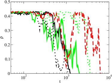
Figure 1: Interface density evolution for individual realizations, for system size $N=10000$ and average connectivity $\left\langle k\right\rangle=8$.

In a disordered configuration with randomly distributed spins $\rho\simeq 1/2$, while when $\rho$ takes a small value it indicates the presence of large spatial domains in which each spin is surrounded by nearest neighbor spins with the same value. For a completely ordered system, that is, for any of the two absorbing states, $\rho=0$. Starting from a random initial condition, the time evolution of $\rho$ describes the kinetics of the ordering process. In regular lattices of dimensionality $d<2$ the system orders. This means that, in the limit of large systems, there is a coarsening process with unbounded growth of spatial domains of one of the absorbing states. The asymptotic regime of approach to the ordered state is characterized in $d=1$ by a power law $\langle\rho\rangle\sim t^{-\frac{1}{2}}$, while for the critical dimension $d=2$ a logarithmic decay is found $\langle\rho\rangle\sim(\ln t)^{-1}$ Dornic01 . Here the average $\langle\cdot\rangle$ is an ensemble average.

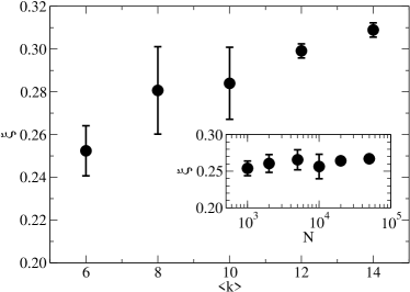
Figure 2: Plateau height for SF networks with different average connectivity. Network size $N=10000$. Inset: Plateau height dependence on network size. Average connectivity $\left\langle k\right\rangle=6$. Data is averaged over $1000$ realizations.

In regular lattices with $d>2$ Krapivsky02 , as well as in small world networks Castellano03 , it is known that the voter dynamics does not order the system in the thermodynamic limit of large systems. After an initial transient, the system falls in these cases in a metastable partially ordered state where coarsening processes have stopped: spatial domains of a given attractor, on the average, do not grow. In the initial transient of a given realization of the process, $\rho$ initially decreases, indicating a partial ordering of the system. After this initial transient $\rho$ fluctuates randomly around an average plateau value $\xi$. This quantity gives a measure of the partial order of the metastable state since $l=\xi^{-1}$ gives an estimate of the average linear size of an ordered domain in that state. In a finite system the metastable state has a finite lifetime: a finite size fluctuation takes the system from the metastable state to one of the two ordered absorbing states. In this process the fluctuation orders the system and $\rho$ changes from its metastable plateau value to $\rho=0$. Considering an ensemble of realizations, the ordering of each of them typically happens randomly with a constant rate. This is reflected in an exponential decay of the ensemble average interface density

$$\left\langle\rho\right\rangle\propto e^{-\frac{t}{\tau}}~{},$$ (3)

where $\tau$ is the survival time of the partially ordered metastable state. Note then that the average plateau value $\xi$ has to be calculated at each time, averaging only over the realization of the ensemble that have not yet decayed to $\rho=0$.

The survival time $\tau$, for a regular lattice in $d=3$ Krapivsky02 and also for a small world network Castellano03 , is known to scale linearly with the system size $N$, $\tau\sim N$, so that the system does not order in the thermodynamic limit. More recently the same scaling has been found for random graphs Redner04 ; Castellano05 while a scaling $\tau\sim N^{0.88}$ has been numerically found Suchecki04 ; Castellano05 for the voter model in the scale free Barabasi-Albert network Barabasi . This scaling is compatible with the analytical result $\tau\sim N/\ln N$ reported in Ref. Redner04 . Other analytical results for uncorrelated networks with arbitrary power law degree distribution are also reported in Ref. Redner04 . We note that a conceptually different, but related quantity, is the time that a finite system takes to reach an absorbing state when coarsening processes are at work. This time $\tau_{1}$ is known to scale as $\tau_{1}\sim N^{2}$ for a regular $d=1$ lattice and $\tau_{1}\sim N\ln N$ for a regular $d=2$ lattice.

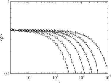
Figure 3: Interface density evolution in SF networks of different sizes (increasing from left to right: $N=1000$, $2000$, $5000$, $10000$, $20000$, and $50000$). Data is averaged over at least $1000$ realizations for $\left\langle k\right\rangle=6$.

In the next sections we discuss the time evolution of $\rho$ and the characteristic properties of the plateau value $\xi$ and survival time $\tau$ for asynchronous node-update voter dynamics in a variety of different complex networks.

III Dimensionality and Ordering: Voter model in scale-free networks

One of simplest models that displays a scale-free degree distributions is the well known Barabasi-Albert network Barabasi . In this model, the degree distribution follows a power law with an exponent $\gamma=3$, the path length grows logarithmically with the system size Albert02 while the clustering coefficient decreases with system size victornet2 . It has been shown that critical phenomena on this class of networks are well reproduced by mean field calculations valid for random networks Goltsev03 . Thus we will consider in the remainder the Barabási-Albert networks as a representative example of a random scale-free (RSF) network. Results for the voter model in the BA network are shown in Figs. 1-3. The qualitative behavior that we observe is the same than the one described above for regular lattices of $d>2$ or also observed in a small world network Castellano03 : The system does not order but reaches a metastable partially ordered state. The interface density $\rho$ for different individual realizations of the dynamics is shown in Fig. 1. In this figure we see examples of how finite size fluctuations take the system from the metastable state with a finite plateau value of $\rho$ to the absorbing state with $\rho=0$. The level of ordering in this finite lifetime metastable state can be quantified by the plateau level $\xi$ shown in Fig. 2. We find that the level of ordering decreases significantly with the average connectivity of the network, a result consistent with the idea that total ordering is more easily achieved for effective lower dimensionality. On the other hand the level of ordering is not seen to be sensitive to the system size, for large enough sizes.

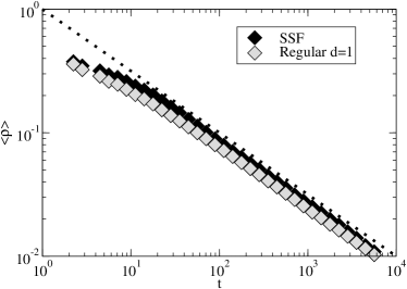
Figure 4: Interface density evolution in one dimensional systems with and without scale-free topology. For reference, the dotted line is a power law with exponent $-\frac{1}{2}$.Average over $1000$ realizations, $N=10000$ and $\left\langle k\right\rangle=8$.

The survival time $\tau$ can be calculated from the ensemble average interface density $\left\langle\rho\right\rangle$ as indicated in Eq. (3). The time dependence of $\left\langle\rho\right\rangle$ for systems of different size (Fig. 3) shows an exponential decrease for which the result mentioned above $\tau\sim N^{0.88}$ can be obtained Suchecki04 . We note that the value $\tau$ is found to be independent of the mean connectivity of the network and that a linear scaling $\tau\sim N$ is obtained if a link update dynamics is used Suchecki04 .

The fact that the presence of hubs in the BA network is not an efficient mechanism to order the system might be counterintuitive, in the same way that the presence of long range links in a small world network is also not efficient to lead to an ordered state. However, in both cases the effective dimensionality of the network is infinity and the result is in agreement with what is known for regular lattices with $d>2$. A natural question is then the relevance of the degree distribution versus the effective dimensionality in the ordering dynamics. To address this question we have chosen to study the voter model dynamics in the Structured Scale Free (SSF) network introduced in Ref. victornet1 . The SSF networks are a nonrandom network with a power law degree distribution with exponent $\gamma=3$ but with an effective dimension $d=1$ Eguiluz03 .

Our results for the time dependence of the average interface density in the SSF network are shown in Fig. 4. For comparison the results for a regular $d=1$ network are also included. For both networks we observe that the system orders with the average interface density decreasing with a power law with characteristic exponent $1/2$

$$\left\langle\rho\right\rangle(t)\sim t^{-\frac{1}{2}}~{}.$$ (4)

The only noticeable difference is that the SSF network has a larger number of interfaces at any moment, but the ordering process follows the same power law. Additionally we find that for a finite systems the time $\tau_{1}$ to reach the absorbing state scales as $\tau_{1}\sim N^{2}$, as it also happens for the regular $d=1$ network:

The network is completely ordered when the last interface disappears. At this point, the density is simply $(N\left\langle k\right\rangle)^{-1}$, where $N\left\langle k\right\rangle$ is the total number of links in the network. Since the interface density decreases $\left\langle\rho\right\rangle\sim t^{-\frac{1}{2}}$, then the time to order $\tau_{1}$ is given by

$$(N\left\langle k\right\rangle)^{-1}=\tau_{1}^{-1/2}~{},$$ (5)

leading to $\tau_{1}\sim N^{2}$.

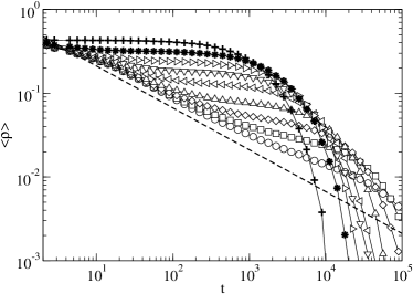
Figure 5: Mean interface density evolution for SWSF networks with different disorder parameter $p$ (increasing from circles to stars: $p=0.0004$, $0.001$, $0.002$, $0.004$, $0.01$, $0.02$, $0.04$, and $0.1$), and comparison with the BA network (+). For reference, the dotted line is a power law with exponent $-\frac{1}{2}$. Data averaged over $100$ realization for $p<0.01$ and over $1000$ realizations for $p\geq 0.01$; $N=10000$ and $\left\langle k\right\rangle=8$.

Therefore we conclude that the effective dimensionality of the network is the important ingredient in determining the ordering process that results from a voter model dynamics, while the fact that the system orders or falls in a metastable state is not sensitive to the degree distribution.

IV Role of network disorder and degree heterogeneity

Once we have identified in the previous section the crucial role of dimensionality we now address the role of network disorder and degree heterogeneity in quantitative aspects of the voter model dynamics. We do that by considering a collection of complex networks in which the system falls into partially disordered metastable states, except for the the regular one-dimensional lattice and SSF networks in which the system shows genuine ordering dynamics:

1. Structured Scale Free (SSF) network as defined in the previous section.

2. Small-World Scale-Free (SWSF) network. This is defined by rewiring with probability $p$ the links of a SSF network. In order to conserve the degree distribution of the unperturbed ($p=0$) networks, a randomly chosen link connecting nodes $i,$ $j$ is permuted with that connecting nodes $k$, $l$) Maslov03 .

3. Random Scale Free (RSF) network: Defined as the limit $p=1$ of the SWSF network. The RSF network shares most important characteristics with the BA network.

   

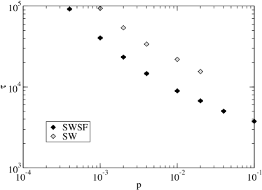
   Figure 6: Survival times for a SWSF network with different disorder parameter $p$. For comparison results for SW networks are also included. Average over $1000$ realizations, $N=10000$ and $\left\langle k\right\rangle=8$.

   By changing the parameter $p$ from $p=0$ (SSF) to $p=1$ (RSF) we can analyze how increasing levels of disorder affect the voter model dynamics while keeping a scale free degree distribution. On the other hand, the consequences of the degree heterogeneity characteristic of SF networks can be analyzed comparing the voter model dynamics on these networks with networks with the same level of disorder and a non-SF degree distribution. These other networks are constructed introducing the same disorder parameter $p$, but starting from a regular $d=1$ network. Namely we consider:

4. Regular $d=1$ network that can be compared with a SSF network.

5. Small World (SW) network defined introducing the rewiring parameter $p$ in the regular network as in the prescription by Watts and Strogatz Watts98 . The SW network can be compared with the SWSF network.

6. Random network (RN) corresponding to the limit $p=1$ of the SW network.

   Likewise, one can consider a random network with an exponential (EN) degree distribution. The EN network is constructed as in the BA prescription but with random instead of preferential attachment of the new nodes. These two random networks, RN and EN, can be compared with the RSF network.

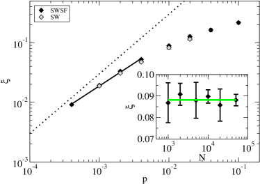
Figure 7: Plateau heights for SWSF networks with different disorder parameter $p$. For reference, dotted line is a power law $\xi\sim p$ while the solid line $\xi\sim p^{0.76}$. For comparison results for SW networks are also included. Average over $100$ realization for $p<0.01$ and over $1000$ realizations for $p\geq 0.01$, $N=10000$ and $\left\langle k\right\rangle=8$. Inset: Plateau heights for SWSF networks of different system size $N$. Average over $1000$ realizations, with $p=0.01$ and $\left\langle k\right\rangle=8$.

IV.1 Role of disorder

Figure 5 shows the evolution of the mean interface density for SWSF networks with different values of the disorder parameter $p$. It shows how varying $p$ one smoothly interpolates between the results for the SSF network and those for a RSF network. In general, increasing network randomness by increasing $p$ the system approaches the behavior in a BA network, making it to to fall in a metastable state of higher disorder, but with finite size fluctuations causing faster ordering. This trend is quantitatively shown in Fig. 6 and Fig. 7 where the the survival time $\tau$ and plateau level $\xi$ for SWSF networks are plotted as a function of the disorder parameter $p$. We observe that $\tau$ and the size of the ordered domains $l=\xi^{-1}$ decrease with $p$ but without following any clear power law. As a general conclusion, when extrapolating to $p=1$, we find that $\tau_{SWSF}>\tau_{RSF}$ and $l_{SWSF}>l_{RSF}$.

The role of increasing disorder in the network can also be analyzed in networks without a scale free degree distribution by considering SW networks with different values of the rewiring parameter $p$. The survival time $\tau$ and plateau level $\xi$ for SW networks are also plotted in Fig. 6 and Fig. 7. We observe that the effect of disorder is qualitatively the same for SW than for SWSF networks powerlawSW . Extrapolating the results in Fig. 6 and Fig. 7 to $p=1$ where the SW network becomes a RN we find that $\tau_{SW}>\tau_{RN}$ and $l_{SW}>l_{RN}$.

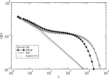
Figure 8: Interface density evolution for SFSW and SW networks with the same level of disorder $p=0.01$. Average over $1000$ realizations, $N=10000$, and $\left\langle k\right\rangle=8$.

IV.2 Role of degree distribution

To address the question of the role of the degree distribution of the network in the voter model dynamics we compare the evolution in networks with a scale free degree distribution with the evolution in equivalent networks but with a degree distribution involving a single scale. A first comparison was already made between the dynamics in a regular $d=1$ network and the SSF network (Fig. 4). This is included for reference in Fig. 8 where we compare the evolution of the mean interface density in a SWSF network with the evolution in a SW network with the same level of disorder. We observe for SWSF a similar plateau value (similar but slightly more disordered state) at any time before the exponential decay of $\langle\rho\rangle$ which is faster for the SWSF than for the SW networks. Finite size fluctuations that order the system seem to be more efficient when hubs are present, causing complete ordering more often, and therefore a faster exponential decay of $\langle\rho\rangle$. These claims are made quantitative in Fig. 6 and Fig. 7 where it is shown that $\tau_{SW}>\tau_{SWSF}$ and $l_{SW}\simeq l_{SWSF}$. In addition, extrapolating to the limit $p=1$ we have that $\tau_{RN}>\tau_{RSF}$ and $l_{RN}\simeq l_{RSF}$

It is also interesting to compare the dependence with system size of the voter model dynamics in SW Castellano03 and SFSW networks: The time dependence of the mean interface density for a SWSF network with an intermediate fixed value of $p$ is shown in (Fig. 9). The qualitative behavior is the same than the one found for SW networks. However, the survival times shown in Fig. 10 deviates consistently from the linear power law $\tau\sim N$ found for SW networks Castellano03 . This deviation might possibly have the same origin than the deviation from the linear power law observed for BA networks, that is the lack of conservation of magnetization in the node-update dynamics of the voter model in a complex network Suchecki04 . This non-conservation becomes much more important in a SWSF network than in a SW network because of the high degree heterogeneity. On the other hand we note that the analytical results for survival times in Ref. Redner04 apply only to uncorrelated networks and therefore do not help us in understanding our numerical result for SWSF networks. We also mention that the plateau level $\xi$ for SWSF networks does not show important dependence with system size (see inset of Fig. 7)

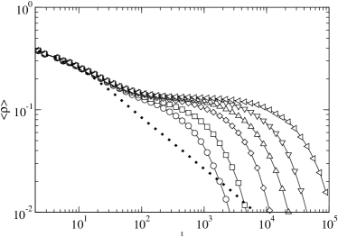
Figure 9: Mean interface evolution for SWSF networks of different system size $N$ (increasing from left to right: $N=1000$, $2000$, $5000$, $10000$, $20000$, $50000$). Average over $1000$ realizations, with $p=0.01$ and $\left\langle k\right\rangle=8$.

The role of degree heterogeneity can be further clarified considering the limit of random networks $p=1$ where the SW network becomes a RN and the SWSF network becomes a RSF network essentially equivalent to the BA network. The evolution for the mean interface density for different random networks is shown in Fig. 11. We find again that when there are hubs (large degree heterogeneity) there is a faster exponential decay of $\langle\rho\rangle$, so that ordering is faster in BA networks than in RN or EN, while the plateau level or level of order in that state does not seem to be sensitive to the degree distribution . This coincides with the extrapolation to $p=1$ of the data in Fig. 6 and Fig. 7 which indicates that $\tau_{RN}>\tau_{RSF}$ and $l_{RN}\simeq l_{RSF}$. Our results for the system size dependence of the survival times and plateau levels for RN and EN networks are shown in Fig. 12. The size of the ordered domains $l=\xi^{-1}$ is again found not to be sensitive to system size. The survival times for RN and EN networks follow a linear scaling $\tau\sim N$ in agreement with the prediction in Ref. Redner04 . We recall that, as discussed earlier, in random networks with scale free distribution such as the BA network a different scaling is found ($\tau\sim N^{0.88}$) Suchecki04 ; Castellano05 compatible with the prediction $\tau\sim N/\ln N$ Redner04 .

Figure 10: Survival times for SWSF networks of different system size $N$. Average over $1000$ realizations, with $p=0.01$ and $\left\langle k\right\rangle=8$.

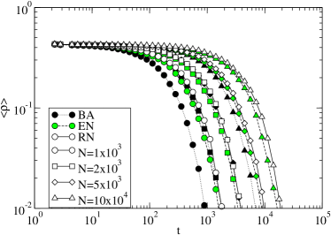
Figure 11: Mean interface density evolution for RN and EN of different sizes $N$. BA network of size $10000$ is also shown for comparison. Average over $1000$ realizations, and $\left\langle k\right\rangle=8$.

V Conclusions

We have analyzed how the ordering dynamics of the voter model is affected by the topology of the network that defines the interaction among the nodes. First we have shown that the voter model dynamics orders the system in a SSF network victornet1 , which is a scale-free network with an effective dimension $d=1$. This result, together with the known result that in regular lattices the voter model orders in $d\leq 2$, suggests that the effective dimension of the underlying network is a relevant parameter to determine whether the voter model orders, but not its degree distribution. The relevance of the effective dimensionality of different scale-free networkshas also been observed in other dynamical processes Eguiluz03 ; Warren02 ; Eguiluz02 ; Klemm03b . In the SSF network the density of interfaces in the voter model decreases as $\langle\rho\rangle\sim t^{-1/2}$ in the same as in the one-dimensional regular lattices.

Second, we have introduced standard rewiring algorithms to study the effect of network disorder. In general we find that network disorder decreases the lifetime of metastable disordered states so that the survival time to reach an ordered state in finite networks is smaller

$$\tau_{SWSF}>\tau_{RSF},\quad\tau_{SW}>\tau_{RS}~{}.$$

Likewise, the average size of ordered domains in these metastable states decreases with increasing disorder

$$l_{SWSF}>l_{RSF},\quad l_{SW}>l_{RS}~{}.$$

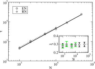
Figure 12: Survival times for RN and EN networks of different sizes $N$. Average over $1000$ realizations, with $\left\langle k\right\rangle=8$. Inset: Plateau heights for the same networks.

Third, the degree heterogeneity also facilitates reaching an absorbing ordered configuration in finite networks by decreasing the survival time: finite size fluctuations ordering the system are more efficient when there are hubsin the network, so that

$$\tau_{SW}>\tau_{SWSF},\quad\tau_{RN}>\tau_{RSF}~{}.$$

The presence of hubs also invalidates the scaling law for the survival time $\tau\sim N$ fouund in SW and RN. However we didn’t appreciate differences in the average size of ordered domains depending on degree heterogeneity

$$l_{SW}\simeq l_{SWSF},\quad l_{RN}\simeq l_{RSF}~{}.$$

In summary, we find for the different classes of networks considered in this work that

$$\tau_{SW}> \tau_{RN} >\tau_{RSF}$$

$$l_{SW}\simeq l_{SWSF}> l_{RN} \simeq l_{RSF}~{}.$$

In general our results illustrate how different features (dimensionality, order, degree heterogeneity) of complex networks modify key aspects of a simple stochastic dynamics.

- (1) J.D. Gunton, M. San Miguel, and P.S. Sahni, in Phase Transitions and Critical Phenomena, Vol 8, pp. 269–466. Eds. C. Domb and J. Lebowitz (Academic Press, London 1983).
- (2) J. Marro and R. Dickman, Nonequilirium Phase Transitions in Lattice Models (Cambridge University Press, Cambridge 1999).
- (3) R. Albert and A.-L. Barabási, Rev. Mod. Phys. 74, 47 (2002).
- (4) Faloutsos, P. Faloutsos, and C. Faloutsos, Computer Communications Rev. 29, 251 (1999).
- (5) M.E.J. Newman and J. Park, Phys. Rev. E 68, 036122 (2003).
- (6) V.M. Eguíluz, D.R. Chialvo, G.A. Cecchi, M. Baliki, and A.V. Apkarian, Phys. Rev. Lett. 94, 018102 (2005).
- (7) A. Aleksiejuk, J. Holyst, and D. Stauffer, Physica A 310, 260 (2002).
- (8) G. Bianconi, cond-mat/0204455 (2002).
- (9) S. N. Dorogovtsev, A. V. Goltsev, and J. F. F. Mendes, Phys. Rev. E 66, 016104 (2002).
- (10) M. Leone, A. Vazquez, A. Vespignani, and R. Zecchina, Eur. Phys. J. B 28,191 (2002).
- (11) D. Boyer and O. Miramontes, Phys. Rev. E 67, 035102(R) (2003).
- (12) V.M. Eguíluz and M.G. Zimmermann, Phys. Rev. Lett. 85, 5659 (2000).
- (13) A. T. Bernardes, D. Satuffer, and J. Kertesz, Eur. Phys. J. B 25, 123 (2002).
- (14) K. Klemm, V.M. Eguíluz, R. Toral, and M. San Miguel, Phys. Rev. E 67, 026120 (2003).
- (15) F. Slanina and H. Lavicka, Eur. Phys. J. B 35, 279 (2003).
- (16) K. Klemm, V.M. Eguíluz, R. Toral, and M. San Miguel, Phys. Rev. E 67, 045101(R) (2003).
- (17) D. Stauffer and H. Meyer-Ortmanns, Int. J. Mode. Phys. C 15, 2 (2003); D. Stauffer, A. O. Sousa, and C. Schulze, JASSS (2004).
- (18) M.G. Zimmermann, V.M. Eguíluz, and M. San Miguel, Phys. Rev. E 69, 065102(R) (2004); V.M. Eguíluz, M.G. Zimmermann, C.J. Cela-Conde, and M San Miguel, Am. J. Socio. 110 (2005) in press.
- (19) T.M. Liggett, Interacting Particle Systems (Springer, New York 1985).
- (20) P.L. Krapivsky, Phys. Rev. A 45, 1067 (1992).
- (21) L. Frachebourg and P.L. Krapivsky, Phys. Rev. E 53, R3009 (1996).
- (22) I. Dornic, H. Chaté, J. Chavé, and H. Hinrichsen, Phys. Rev. Lett. 87, 045701 (2001).
- (23) K. Klemm and V.M. Eguíluz, Phys. Rev. E 65, 036123 (2002).
- (24) D.J. Watts and S.H. Strogatz, Nature 393, 440 (1998).
- (25) K. Suchecki, V. M. Eguíluz, and M. San Miguel, Europhysics Letters 69, 228 (2005).
- (26) F. Wu and B. A. Huberman, cond-mat/0407252 (2004).
- (27) C. Castellano, D. Vilone, and A. Vespignani, Europhysics Letters 63, 153 (2003).
- (28) D. Vilone, and C. Castellano, Phys. Rev. E 69, 016109 (2004)
- (29) V. Sood and S. Redner, cond-mat/0412599 (2004).
- (30) C. Castellano, V. Loreto, A. Barrat, and F. Cecconi, and D. Parisi, cond-mat/0501599.
- (31) K. Klemm, V.M. Eguíluz, Phys. Rev. E 65, 057102 (2002).
- (32) A. L. Barabási and R. Albert, Science 286, 509 (1999).
- (33) A.V. Goltsev, S.N. Dorogovtsev, and J.F.F. Mendes, Phys. Rev. E 67, 026123 (2003).
- (34) V. M. Eguíluz, E. Hernández-García, O. Piro, and K. Klemm, Phys. Rev. E 68, 055102(R) (2003).
- (35) The power law dependence of on reported previously in Ref. Vilone04 for SW networks is included for reference in Fig. 7, but seems to be valid only for very small values of .
- (36) S. Maslov, K. Sneppen, and U. Alon, in Handbook of Graphs and Networks, edited by S. Bornholdt and H. G. Schuster, (Wiley-VCH and Co., Weinheim, 2003).
- (37) C.P. Warren, L.M. Sander, and I.M. Sokolov, Phys. Rev. E 66, 056105 (2002).
- (38) V.M. Eguíluz and K. Klemm, Phys. Rev. Lett. 89, 108701 (2002).
- (39) K. Klemm, V.M. Eguíluz, R. Toral, and M. San Miguel, Phys. Rev. E 67, 026120 (2003).