Spin-glass behavior in the random-anisotropy Heisenberg model

Abstract

We perform Monte Carlo simulations in a random anisotropy magnet at a intermediate exchange to anisotropy ratio. We focus on the out of equilibrium relaxation after a sudden quenching in the low temperature phase, well below the freezing one. By analyzing both the aging dynamics and the violation of the Fluctuation Dissipation relation we found strong evidence of a spin–glass like behavior. In fact, our results are qualitatively similar to those experimentally obtained recently in a Heisenberg-like real spin glass.

I Introduction

Random magnetic anisotropy seems to be a fundamental ingredient for any realistic description of amorphous materials, which are systems of both practical and theorical relevancy. For the particular case of amorphous alloys Hellman98PRB ; Pickart74PRL of non-S-state rare earths and transition metals (RE-TM), such as Tb_xFe_1-x, the three dimensional classical Heisenberg model with random uniaxial single-site anisotropy (RAM) is considered to be the proper model for studying both their thermodynamic and dynamic properties. This model was introduced by Harris, Plischke, and Zuckermann, Harris73PRL who performed a mean-field calculation and found a ferromagnetic (FM) phase at low temperature. Later on, Pelcovits, Pytte and Rudnick Pelcovits78PRL claimed, using an argument similar to that used by Imry and Ma Imry75PRL for the random-field case, that such a FM phase is not stable in three dimensional RAM model, for any finite value of the anisotropy. Since then, the nature of the ordered phase at low temperatures and its dependence on the degree of anisotropy is a subject of controversy. Recently, Itakura Itakura03PRB proposed, by using Monte Carlo simulations and referring to former works in the literature, a schematic phase diagram for the RAM where different kinds of order can be found, depending both on the temperature and the anisotropy strength of the system.

When an amorphous material is cooled, it can eventually get blocked at certain temperature $T_{f}$, at which the magnetic moments freeze pointing in random directions. The value of $T_{f}$ strongly depends on the degree of anisotropy, the strength of the interactions between domains and the cooling rate. It is worth here to stress that this freezing process is a dynamical phenomenon which can not be associated to any true thermodynamical phase transition. In particular, this phenomenology has been reported, during the last years, in the study of hard magnetic amorphous alloys Inoue96JIM ; Billoni03JMMM , which has been also successfully simulated using a slightly modified version of the RAM Wang01PRB . On the other hand, in experimental spin glasses Chamberlin82PRB , zero field cooling (ZFC) and field cooling (FC) curves of magnetization versus temperature are useful to estimate the characteristic freezing temperatures of the systems.

Most of the numerical effort in the study of the RAM model concerns the case of strong or infinite anisotropy. In this case the model seems to present a low temperature spin glass like phase (usually called speromagnetic Coey78JAP ). On the other hand, in the weak anisotropy limit, the system tends to order locally in a ferromagnetic state Chudnovsky86PRB (also called asperomagnetic). When increased to intermediate values,the anisotropy seems to destroy the asperomagnetic ferromagnetic state, and the systems orders in the so called correlated speromagnetic or correlated spin–glass. It has been recently verified in Ref.Itakura03PRB , by means of a very extensive numerical simulation, that the competition between exchange and anisotropy gives place to a quasi–long–range order (QLRO) low temperature phase characterized by frozen power–law spin–spin correlations. It is important here to remark that all the theoretical results ultimately confirm the observed lack of long range ferromagnetic order observed experimentally in magnetic materials with isotropic easy axis distribution Dudka04CM .

Although the RAM model has deserve much attention during the last years, most of the works were concerned on its equilibrium properties as well as on its magnetic behavior, paying little attention to its relaxation dynamics. The main question we want to address in this work concerns the possible existence of a spin–glass like dynamical behavior associated with QLRO low temperature phase in the intermediate anisotropy regime. We analyze, through Monte Carlo simulations, the out of equilibrium relaxation of the three dimensional RAM model defined on a cubic lattice. In particular, we report results obtained in the low temperature phase (well below $T_{f}$) and for intermediate values of the anisotropy to exchange ratio.

II The model

The system is ruled by the following classical Heisenberg Hamiltonian:

$$H=-J\sum_{<i,j>}\vec{S}_{i}\cdot\vec{S}_{j}-D\sum_{i}(\vec{n}_{i}\cdot\vec{S}_{i})^{2}-\vec{H}_{i}\cdot\vec{S}_{i}$$ (1)

where $D$ and $J>0$ are the anisotropy and the exchange strength, respectively, and $\vec{H}_{i}$ is an external field acting on the site $i$. The spin variable $\vec{S}_{i}$ is a three components unit vector associated to the $i$–th node of the lattice and the first sum runs over all nearest-neighbor pairs of spins. $\vec{n}_{i}$ is unit random vector that defines the local easy axis direction of the anisotropy at site $i$. These easy axis are quenched variables chosen from a isotropic distribution on the unit sphere. The simulations were performed in a system of $N=L^{3}$ spins ($L=15$), using a Monte Carlo Metropolis algorithm GarciaOtero99JAP with periodic boundary conditions (in fact, we have compare different system sizes up to $L=20$, confirming that for $L=15$ finite size effects become very small). The ratio between the anisotropy and the exchange strength was fixed at the value $D/J=3.5$, which is comparable to those values observed in real amorphous material and clusters ferromagnetic alloys Wang01PRB . Following the ideas used in Ref. Wang01PRB , at each spin actualization the direction of the spin is adjusted in such a way to maintain an acceptation rate close to 0.46.

III Results

The first step was to locate the freezing temperature $T_{f}$ for these particular values of the parameters by looking for the temperature at which zero field cooling (ZFC) and field cooling (FC) curves split each other. Fig.1 shows the magnetization divided by the field $M/H$ (dc susceptibility) as a function of $T/J$, both for the ZFC and FC processes. The simulation protocol used is the following: we performed 1000 Monte Carlo steps (MCS) at a given temperature and at a constant acceptance rate in order to equilibrate the system, after which, we used other 1000 MCS to get a time average of the magnetization before decreasing the temperature. In all the simulations presented in this work we have used between 20 and 40 different realizations of the disorder to average the results. We find that the freezing temperature $T_{f}/J$ is close to $0.5$. At very low temperature the dc susceptibility in the ZFC curves is constant and the magnetization almost zero, indicating a speromagnetic spin–glass like order. In other words, the spins are frozen into random orientations with average correlation over at most one lattice parameter (we have verified this behavior by calculating the dependence of the spin-spin correlation function as function of the distance). As temperature increases the dc susceptibility also increases, indicating that the system goes to an anisotropic asperomagnetic phase. Here again, the same conclusion has been verified by analyzing the correlation function which stabilizes in a non zero value for distances larger than approximately four lattice units.

On the other hand, it can be seen that as $T\to 0$, $M_{FC}\to 0.5$, as expected in an asperomagnetic phase (and in agreement with other theoretical Chudnovsky86PRB and numerical predictions Harris78JPFMP ). Due to local character of this asperomagnetic phase, a sufficiently large system could eventually develop a local order without any global magnetization (QLRO), as in fact is observed in amorphous materials. Notice that both curves present, above $T_{f}$, an inflection point which is very close to the Heisenberg critical temperature, indicating the loss of magnetic order and the entrance in the paramagnetic phase (or superparamagnetic phase, in particulate systems). It is worth here to remark that the FC curves display a clear cusp, that closely resembles the experimental results obtained in spin glasses, as for intance in AgMn Chamberlin82PRB , confirming the random freezing of the spin orientations.

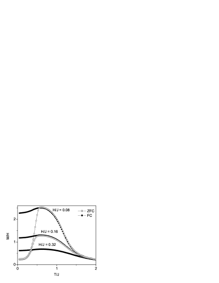
Figure 1: Magnetization divided by the field $M/H$ (dc susceptibility) as a function of the rescaled temperature $T/J$ for different applied fields, both for the ZFC and FC processes.

Disordered systems, when suddenly quenched down into the low temperature phase, suffer a drastic slowing down of their relaxation dynamics. At the same time, a very strong dependence on the history of the sample emerges, a phenomenon usually called aging. In a real experiment, the simplest way for measuring aging is by suddenly quenching the system without field into the ordered phase. The system ages in this phase during certain waiting time $t_{w}$, at which the field is switched off. The measurement of the relaxation of the magnetization then strongly depends on both, the age or waiting time $t_{w}$ and the time $t$ elapsed since the field was turned off, indicating the loss of time translation invariance (TTI) proper of any equilibrated state. In a computer simulation the same effect can be visualized by measuring the two time auto correlation function after a sudden quench from infinite temperature into the low temperature phase:

$$C(t+t_{w},t_{w})=\left[\frac{1}{N}\sum_{i}\left<\vec{S}_{i}(t_{w})\cdot\vec{S}_{i}(t+t_{w})\right>\right]$$ (2)

where $t_{w}$ is the time elapsed after the quenching and $[\cdots]$ means an average over the disorder.

Figure 2: Correlation curves $C(t_{w}+t,t_{w})$ as function of time $t$ (MCS) obtained at $T/J=0.2$, for $L=15$ and for different values of $t_{w}$.

In Fig. 2 we present the curves of $C(t_{w}+t,t_{w})$ obtained at $T/J=0.2$, $L=15$ and for different values of $t_{w}$. The plot clearly confirms the appearance of aging, characterized both by the loss of TTI and the fact that the system decays slower as its age $t_{w}$ increases.

Actually, aging is so ubiquitous in nature, that one can wander whether it is useful or not to look for this phenomenology. But fortunately, the peculiar dependence of $C(t_{w}+t,t_{w})$ on $t$ and $t_{w}$ on a great variety of systems (both theoretical and real systems) suggests the existence of only a few universality classes associated to the out of equilibrium relaxation of the model, as occurs, for instance, in critical phenomena and coarsening dynamics. All this indicates that, despite any microscopic difference between different systems, the relaxation must be dominated by a few relevant ingredients.

Figure 3: Rescaled correlations curves for three different values of $T/J$ ($0.1$, $0.15$ and $0.2$). Each curve we shown in the graph correspond to four correlation curves $C(t_{w}+t,t_{w})$ with $t_{w}=5000$, $10000$, $20000$ and $40000$ (measured in MCS).

In order to classify the universality class, we looked for the best data collapse of the curves obtained for different waiting times, checking different scaling forms. The best results we obtained are presented in Figure 3, where we followed the standard scaling procedure used in spin glasses materials (like for instance CdIn_0.3Cr_1.7S₄ Alba87JAP ). The two time autocorrelation function is assumed to have two different components $C(t_{w}+t,t_{w})=C_{st}(t)+C_{ag}(t_{w}+t,t_{w})$, the first one corresponding to an stationary part (independent of $t_{w}$) and the second part (the aging one) depending both on $t$ and $t_{w}$. The stationary part is a power law function $A(\tau_{0}/t)^{\alpha}$, which is predominant at very small times. The aging part is a function of $\lambda(t,t_{w})/t_{w}$, where

$$\lambda=t_{w}[(1+t/t_{w})^{1-\mu}-1]/[1-\mu]$$ (3)

The curves presented in Fig.3 correspond to three different values of $T/J$ ($0.1$, $0.15$ and $0.2$), all of them well below the freezing temperature of the system. In each curve we have collapsed the four different curves obtained for four different waiting times $t_{w}=5000$, $10000$, $20000$ and $40000$ (measured in MCS). Note the excellent superpositions obtained, which extends over the complete time span simulated. It is worth to stress that this scaling law has been vastly used in the study of aging dynamics in real spin glass materials, yielding excellent data collapses of the experimental results Vincent87JPC ; Ladieu04CM ; Alba87JAP ; Vincent97SV .

The set of fitting parameters obtained (shown in table 1) are in a good agreement with those obtained experimentally in real spin glasses Alba87JAP . This behavior indicates that $C(t_{w}+t,t_{w})$ scales as $t/t_{w}^{\mu}$ at short $t$ (since $\mu<1$), while in the large $t$ limit and for the values of $\mu$ obtained (which are all close to 1) its behaviors is almost logarithmic on $t/t_{w}$ (as expected in a activated scenario Fisher88PRB ).

Table 1: Fitting parameters of the scaling.

$T/J$	$A$	$\alpha$	$\mu$
0.10	0.002	0.4	0.93
0.15	0.012	0.06	0.86
0.20	0.16	0.07	0.83

Finally, we analyzed the Fluctuation Dissipation Relation (FDR), which can be expressed as Cugliandolo93PRL :

$$R(t_{w}+t,t_{w})=\frac{X(t_{w}+t,t_{w})}{3T}\frac{\partial C(t_{w}+t,t_{w})}{\partial t_{w}}$$ (4)

where $R(t_{w}+t,t_{w})=1/N\;\sum_{i}\partial\left<S_{i}^{z}(t_{w}+t)\right>/\partial h_{i}(t_{w})$ is the response to an external magnetic field $h_{i}(t)$ in the $z$ direction and $X(t_{w}+t,t_{w})$ is the fluctuation dissipation factor. In equilibrium the Fluctuation Dissipation Theorem (FDT) holds and T $X(t_{w}+t,t_{w})=1$, while out of equilibrium $X$ depends on $t$ and $t_{w}$ in an non trivial way. It has been conjectured Cugliandolo93PRL that $X(t_{w}+t,t_{w})=X[C(t_{w}+t,t_{w})]$. This conjecture has proved valid in all systems studied to date.

Instead of considering the response function it is easier to analyze the integrated response function

$$\chi(t_{w}+t,t_{w})=\int_{t_{w}}^{t_{w}+t}R(t_{w}+t,s)\,ds.$$ (5)

Assuming $X(t_{w}+t,t_{w})=X[C(t_{w}+t,t_{w})]$ one obtains

$$3\,T\chi(t_{w}+t,t_{w})=\int_{C(t_{w}+t,t_{w})}^{1}X(C)dC$$ (6)

and by plotting $3\,T\,\chi$ vs. $C$ one can extract $X$ from the slope of the curve. In particular, if the FDT holds $X=1$ and $3\,T\chi(t)=(1-C(t))$; any departure from this straight line brings information about the non-equilibrium process. In numerical simulations of spin glass Parisi98PRB and structural glass models Kob97PRL ; Parisi97PRL it has been found that, in the non-equilibrium regime, this curve follows another straight line with smaller (in absolute value) slope when $t/t_{w}\gg 1$. In this case the FD factor $X$ can be interpreted as an effective inverse temperature Cugliandolo97PRE $T_{eff}=T/X$. At time $t_{w}$ we took a copy of the system spin configuration, to which a random magnetic field $h_{i}(t)=h\,\epsilon_{i}$ was applied, in order to avoid favoring the QLRO Barrat98PRE ; Stariolo99PRB ; $\epsilon_{i}$ was taken from a bimodal distribution ($\epsilon_{i}=\pm 1$). Using the results from the FC and ZFC calculations, the strength $h$ of the field was taken small enough to guarantee linear response; the integrated response then equals $\chi(t_{w}+t,t_{w})=m(t_{w}+t,t_{w})/h$, where $m(t_{w}+t,t_{w})$ is the staggered magnetization conjugated to the field $h_{i}(t)$, averaged over the random field variables.

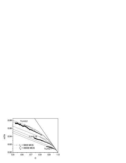
Figure 4: Parametric plot of $T\,m(t+t_{w},t_{w})/h$ versus $C(t+t_{w},t_{w})$ for three reduced temperatures $T/J$ ($0.1$, $0.15$ and $0.2$ from bottom to top) and two different waiting times $t_{w}$ ($5000$ and $40000$ MCS). The solid line indicates the validity of Fluctuation Dissipation Theorem (slope $1/3$).

In Fig. 4 we display $T\,m(t_{w}+t,t_{w})/h$ vs. $C(t_{w}+t,t_{w})$ in a parametric plot. The curves correspond to the three different values of $T/J$ plotted in Fig. 3; in each case we present the results obtained for two different waiting times $t_{w}=5000$ and $40000$ MCS. In all the cases studied we observe a typical two time scale separation behavior, proper of real spin glasses. At $t=0$ the system starts in the right bottom corner (fully correlated and demagnetized) and during certain time (that depends in this case both on $t_{w}$ and $\mu$) it runs over the equilibrium straight line, indicating the existence of a quasi equilibrium regime. Nevertheless, at certain time the system clearly departures from this quasi–equilibrium curve and moves along a different straight line, but with a different (smaller) slope, indicating an effective temperature that is larger than the temperature of the thermal bath. This one–step temporal regime observed in this model is very common in structural glasses but also in spin glass materials. Both numerical results on the Heisenberg spin glass with weak anisotropy Kawamura03PRL and experimental measurements in CdIn_0.3Cr_1.7S₄ spin glasses, present this kind of dynamical behavior.

IV Conclusions

In this paper we have studied the out of equilibrium dynamics of the RAM model. The parameters have been chosen in such a way to model systems with a freezing temperature well below the ordering temperature. We have restricted ourselves to consider the case of intermediate values of $D/J$, where both effects exchange and randomness, compete with each other. This peculiar regime is specially interesting, since on one hand there exists certain degree of controversy about the expected ordering of the system, and on the other hand it allows to model different interesting real magnetic materials. Our analysis, based the study of ZFC-FC curves, aging and on the FDR in the low temperature phase, are consistent with the existence of a spin–glass ground state of the model, where the slowing mechanisms are then related to the topology of the energy landscape of the model.

This work was partially supported by grants from CONICET (Argentina), Agencia Córdoba Ciencia (Argentina) and SECYT/UNC (Argentina).

References

- (1) F. Hellman, E. N. Abarra, A. L. Shapiro, and R. B. van Dover, Phys. Rev. B 58, 5672 (1998).
- (2) S. J. Pickart, J. J. Rhyne, and H. A. Alperin, Phys. Rev. Lett. 33, 424 (1974).
- (3) R. A. Pelcovits, E. Pytte, and J. Rudnick, Phys. Rev. Lett. 40, 476 (1978).
- (4) Y. Imry and S. K. Ma, Phys. Rev. B 35, 1399 (1975).
- (5) R. Harris, M. Plischke, and M. J. Zuckermann, Phys. Rev. Lett. 31, 160 (1973).
- (6) M. Itakura, Phys. Rev. B 68, 100405(R) (2003).
- (7) A. Inoue, T. Zhang, and A. Takeuchi, Mater. Trans. JIM 37, 99 (1996).
- (8) O. Billoni, S. Urreta, and L. Fabietti, J. Magn. Magn. Mater. 265, 222 (2003).
- (9) L. Wang, J. Ding, H. Z. Kong, Y. Li, Y. P. Feng, Phys. Rev. B 64, 214410 (2001).
- (10) R. V. Chamberlin, M. Hardiman, L. A. Turkevich, and R. Orbach, Phys. Rev. B 25, 6720 (1982).
- (11) J.M.D. Coey, J. Appl. Phys. 49, 1646 (1978).
- (12) E. M. Chudnovsky, W. M. Saslow, and R. A. Serota, Phys. Rev. B 33, 251 (1986).
- (13) M. Dudka, R. Folk, and Y. Holovatch, Cond–Mat/0406692 (2004).
- (14) J. García-Otero, M. Porto, J. Rivas, and A. Bunde, J. Appl. Phys. 85, 2287 (1999).
- (15) R. Harris and S. H. Sung, Journal of Physics F: Metal Physics 8, L299 (1978).
- (16) E. Vincent and J. Hammann, J. Phys. C 20, 2659 (1987).
- (17) F. Ladieu, F. Bert, V. Dupuis, E. Vincent, and J. Hammann, Cond–Mat/0403356 (2004).
- (18) M. Alba et al., J. Appl. Phys. 63, 3683 (1987).
- (19) E. Vincent, J. Hammann, M. Ocio, JP Bouchaud and L. Cugliandolo, Proceedings of the Sitges conference (E. Rubi ed, Springer-Verlag, 1997)
- (20) D. S. Fisher and D. A. Huse, Phys. Rev. B 38, 386 (1988).
- (21) L. F. Cugliandolo and J. Kurchan, Phys. Rev. Lett. 71, 173 (1993).
- (22) G. Parisi, F. Ricci-Tersenghi, and J. J. Ruiz-Lorenzo, Phys. Rev. B 57, 13617 (1998).
- (23) W. Kob and J.-L. Barrat, Phys. Rev. Lett. 78, 4581 (1997).
- (24) G. Parisi, Phys. Rev. Lett. 79, 3660 (1997).
- (25) L. F. Cugliandolo, J. Kurchan, and L. Peliti, Phys. Rev. E 55, 3898 (1997).
- (26) A. Barrat, Phys. Rev. E 57, 3629 (1998).
- (27) D. A. Stariolo and S. A. Cannas, Phys. Rev. B 60, 3013 (1999).
- (28) H. Kawamura, Phys. Rev. Lett. 90, 237201 (2003).