Thermodynamics of $S\geqslant 1$ ferromagnetic Heisenberg chains with uniaxial single-ion anisotropy

Abstract

The thermodynamic properties of $S\geqslant 1$ ferromagnetic chains with an easy-axis single-ion anisotropy are investigated at arbitrary temperatures by both a Green-function approach, based on a decoupling of three-spin operator products, and by exact diagonalizations of chains with up to $N=12$ sites using periodic boundary conditions. A good agreement between the results of both approaches is found. For the $S=1$ chain, the temperature dependence of the specific heat reveals two maxima, if the ratio of the anisotropy energy $D$ and the exchange energy $J$ exceeds a characteristic value, $D/J>7.4$, and only one maximum for $D/J<7.4$. This is in contrast to previous exact diagonalization data for comparably small chains ($N\leqslant 7$) using open boundary conditions. Comparing the theory with experiments on di-bromo Ni complexes the fit to the specific heat yields concrete values for $D$ and $J$ which are used to make predictions for the temperature dependences of the spin-wave spectrum, the correlation length, and the transverse magnetic susceptibility.

I INTRODUCTION

In low-dimensional spin systemsSRF04 the interplay of quantum and thermal fluctuations and the effects of spin anisotropies on the thermodynamics are of basic interest. Whereas for Heisenberg antiferromagnets quantum fluctuations occur already at $T=0$, in ferromagnets, possibly with an easy-axis anisotropy, quantum fluctuations exist at nonzero temperatures only. The study of systems with ferromagnetic exchange couplings, e.g., of the quasi-one-dimensional (1D) $S=1$ ferromagnet CsNiF₃ with an easy-plane single-ion anisotropy,KV87 is also motivated by the progress in the synthesis of new low-dimensional materials, such as the frustrated $S=\frac{1}{2}$ quasi-1D cuprates.Mat04 Likewise, the magnetic behavior of LaMnO₃, a parent compound of the colossal magnetoresistance manganites,Ram97 may be described by an effective spin $S=2$ model with a ferromagnetic intraplane and an antiferromagnetic interplane coupling, where neutron-scattering experimentsMou96 yield evidence for a pronounced ferromagnetic short-range order (SRO) in the paramagnetic phase and for an easy-axis single-ion anisotropy. To provide a good analytical description of SRO and of the thermodynamics at arbitrary temperatures, the standard spin-wave approaches cannot be adopted. Recently, the Green-function equation of motion decoupling of second order and the Green-function projection method with a two-operator basis, respectively,KY72 ; RS73 ; ST91 ; SSI94 ; WI97 ; ISF01 ; JIR04 ; SRI04 have been successfully applied to quantum spin systems with anisotropies of different kind, where most of the previous work was devoted to $S=\frac{1}{2}$ systems and only in Refs. RS73, and SSI94, low-dimensional isotropic $S\geqslant 1$ ferromagnets have been considered. However, the study of anisotropic $S\geqslant 1$ magnets is of current interest.GJL92 ; Pot71 ; FJK00 ; FKS02 In Refs. Pot71, ; FJK00, ; FKS02, the $S=1$ ferromagnet with an easy-axis single-ion anisotropy was investigated in the random phase approximation (RPA) for the exchange term. By this approach the paramagnetic phase and its SRO properties cannot be described. Therefore, a second-order Green-function theory of SRO for anisotropic $S\geqslant 1$ models, going one step beyond the RPA, should be developed.

As a first step in this direction, we present a theory for the $S\geqslant 1$ ferromagnetic chain with an easy-axis single-ion anisotropy described by the model

$$H=-\frac{J}{2}\sum_{\langle i,j\rangle}\bm{S}_{i}\bm{S}_{j}-D\sum_{i}(S_{i}^{z})^{2}$$ (1)

[$\langle i,j\rangle$ denote nearest-neighbor (NN) sites] with $J>0,\;D>0$, and $\bm{S}_{i}^{2}=S(S+1)$. The choice $D>0$ is motivated by our emphasis on the temperature dependence of the specific heat, which reveals a double maximum being more pronounced for $D>0$ than for $D<0$,BLO75 and by the comparison with the experiments on di-bromo Ni complexesKBD74 which may be described by the model (1) with $D>0$.

Furthermore, we perform exact finite-lattice diagonalizations (ED) of $S=1$ chains with up to $N=12$ sites using periodic boundary conditions which are critically analyzed in relation to the ED results by BlöteBLO75 for the specific heat using open boundary conditions.

The paper is organized as follows. In Sec. II the second-order Green-function theory for the model (1) is developed extending previous approaches for $S=\frac{1}{2}$ (Refs. KY72, ; ST91, ; WI97, ; ISF01, ; JIR04, ; SRI04, ) to $S\geqslant 1$ and rotation-invariant methods for $S\geqslant 1$ (Refs. RS73, and SSI94, ) to the case of an easy-axis on-site anisotropy. To test the theory, in Sec. III the limiting cases $J=0$ and $D=0$ are considered in comparison with exact and ED results. The effects of spin anisotropy are explored in Sec. IV. The spin-wave spectrum, the spin susceptibility, and the specific heat are investigated with the focus on the condition for the existence of two maxima in the temperature dependence of the specific heat. Moreover, the theory is compared with available experimental data, and predictions for some relevant quantities are made. A summary of our work can be found in Sec. V.

II GREEN-FUNCTION THEORY

The dynamic spin susceptibilities $\chi_{q}^{\nu\mu}(\omega)=-\langle\langle S_{q}^{\nu};S_{-q}^{\mu}\rangle\rangle_{\omega}\;\;(\nu\mu=+-,zz;\;-\pi\leqslant q\leqslant\pi)$, defined in terms of two-time retarded commutator Green functions, EG79 are determined by the projection method. WI97 ; ISF01 ; JIR04 Taking into account the breaking of rotational symmetry by the single-ion spin anisotropy we choose, as in Refs. ISF01, and JIR04, , the two-operator basis $\bm{A}^{\nu}=(S_{q}^{\nu},i\dot{S}_{q}^{\nu})^{T}\;\;(\nu=+,z)$. Because the model considered has up-down symmetry with respect to $S_{i}^{z}\rightarrow-S_{i}^{z}$, we have $\langle S_{i}^{z}\rangle=0$. Neglecting the self-energy, the matrix Green function $\langle\langle\bm{A};\bm{A}^{+}\rangle\rangle_{\omega}=[\omega-\bm{M}^{\prime}\bm{M}^{-1}]^{-1}\bm{M}$ with the moment matrices $\bm{M}=\langle[\bm{A},\bm{A}^{+}]\rangle$ and $\bm{M}^{\prime}=\langle[i\dot{\bm{A}},\bm{A}^{+}]\rangle$ yields

$$\chi_{q}^{\nu\mu}(\omega)=-\frac{M_{q}^{\nu\mu}}{\omega^{2}-(\omega_{q}^{\nu\mu})^{2}},\;\;\;(\omega_{q}^{\nu\mu})^{2}=M_{q}^{(3)\nu\mu}/M_{q}^{\nu\mu},$$ (2)

where $M_{q}^{\nu\mu}=\langle[i\dot{S}_{q}^{\nu},S_{-q}^{\mu}]\rangle$ and $M_{q}^{(3)\nu\mu}=\langle[-\ddot{S}_{q}^{\nu},-i\dot{S}_{-q}^{\mu}]\rangle$. The first spectral moments are given by the exact expressions

$$M_{q}^{+-}=4JC_{1}(1-\cos q)+2D[3C_{0}^{zz}-S(S+1)],$$ (3)

$$M_{q}^{zz}=2JC_{1}^{+-}(1-\cos q).$$ (4)

The correlation functions $C_{n}=\frac{1}{2}C_{n}^{+-}+C_{n}^{zz}$ and $C_{n}^{\nu\mu}=\langle S_{0}^{\nu}S_{n}^{\mu}\rangle=\frac{1}{N}\sum_{q}C_{q}^{\nu\mu}\text{e}^{iqn}$ with $C_{q}^{\nu\mu}=\langle S_{q}^{\nu}S_{-q}^{\mu}\rangle$ are calculated by the spectral theorem, EG79 analogous to Ref. JIR04, , as

$$C_{q}^{\nu\mu}=\frac{M_{q}^{\nu\mu}}{2\omega_{q}^{\nu\mu}}[1+2n(\omega_{q}^{\nu\mu})]+D_{q}^{\nu\mu},$$ (5)

$$D_{q}^{\nu\mu}=\lim_{\omega\to 0}\frac{\omega}{2}\langle\langle S_{q}^{\nu};S_{-q}^{\mu}\rangle\rangle_{\omega}^{(+)},$$ (6)

where $n(\omega)=(\text{e}^{\omega/T}-1)^{-1}$ and $\langle\langle\cdots;\cdots\rangle\rangle^{(+)}$ denotes the anticommutator Green function. The on-site correlators $C_{0}^{\nu\mu}$ are related by the sum rule

$$C_{0}^{+-}+C_{0}^{zz}=S(S+1)$$ (7)

which follows from the operator identity $\bm{S}_{i}^{2}=S_{i}^{+}S_{i}^{-}-S_{i}^{z}+(S_{i}^{z})^{2}$ and $\langle S_{i}^{z}\rangle=0$.

To obtain the spectra $\omega_{q}^{\nu\mu}$ in Eq. (2) in terms of two-spin correlation functions we approximate the time evolution of the spin operators $-\ddot{S}_{q}^{\nu}$ in the spirit of the schemes proposed in Refs. KY72, ; RS73, ; ST91, ; SSI94, ; WI97, ; ISF01, ; JIR04, . That is, taking the site representation the products of three spin operators in $-\ddot{S}_{i}^{\nu}$ are expressed in terms of one spin operator. Then, the projection method neglecting the self-energy becomes equivalent to the equation of motion decoupling in second order.

In $-\ddot{S}_{i}^{+}$ we decouple the operators along NN sequences $\langle i,j,l\rangle$ as JIR04

$$S_{i}^{+}S_{j}^{+}S_{l}^{-}=\alpha^{+-}\langle S_{j}^{+}S_{l}^{-}\rangle S_{i}^{+}+\alpha^{+-}\langle S_{i}^{+}S_{l}^{-}\rangle S_{j}^{+}.$$ (8)

Here, following the investigation of the isotropic ferromagnet, ST91 ; SSI94 the dependence on the relative site positions of the vertex parameters (cf. Ref. WI97, ) is neglected.

For $S\geqslant 1$, in $-\ddot{S}_{i}^{+}$ there appear products of three spin operators with two coinciding sites which we decouple as proposed in Refs. RS73, and SSI94, ,

$$S_{i}^{+}S_{j}^{-}S_{j}^{+}=\langle S_{j}^{-}S_{j}^{+}\rangle S_{i}^{+}+\lambda^{+-}\langle S_{i}^{+}S_{j}^{-}\rangle S_{j}^{+}.$$ (9)

Furthermore, for $D\neq 0,\;-\ddot{S}_{i}^{+}$ contains the term $D^{2}A_{i}$ with

$$A_{i}\equiv S_{i}^{+}(S_{i}^{z})^{2}+2S_{i}^{z}S_{i}^{+}S_{i}^{z}+(S_{i}^{z})^{2}S_{i}^{+}.$$ (10)

For $S=\frac{1}{2}$ we have $A_{i}=0$, and for $S=1$ we get $A_{i}=S_{i}^{+}$ (Ref. FKS02, ) using the relation $(S_{i}^{z})^{2}S_{i}^{+}=S_{i}^{z}S_{i}^{+}$ (Ref. JA00, ). To obtain a reasonable approximation of $A_{i}$ for $S>1$, we calculate exactly the average $\langle A_{i}S_{i}^{-}\rangle(T)$ at $T=0$ and $T\rightarrow\infty$. We obtain $\langle A_{i}S_{i}^{-}\rangle(0)=(2S-1)^{2}\langle S_{i}^{+}S_{i}^{-}\rangle(0)$ with $\langle S_{i}^{+}S_{i}^{-}\rangle(0)=C_{0}^{+-}(0)=S$ and $\lim_{T\to\infty}\langle A_{i}S_{i}^{-}\rangle=\frac{1}{5}[4S(S+1)-3]\lim_{T\to\infty}\langle S_{i}^{+}S_{i}^{-}\rangle$ with $\lim_{T\to\infty}\langle S_{i}^{+}S_{i}^{-}\rangle=\frac{2}{3}S(S+1)$. Due to those results, for $S>1$ we approximately replace $A_{i}$ by

$$A_{i}=\eta(2S-1)^{2}S_{i}^{+}$$ (11)

with $\eta(T=0)=1$ and $\eta(T\rightarrow\infty)=\frac{4S(S+1)-3}{5(2S-1)^{2}}$. Note that Eq. (11) holds exactly for $S=1$ with $\eta(T)=1$. Considering the ratio $R\equiv\eta/C_{0}^{zz}$, for$S=2\;(3)$ we have $\lim_{T\to\infty}R=0.23\;(0.09)$ as compared with $R(0)=S^{-2}=0.25\;(0.11)$. Accordingly, for $1<S\leqslant 3,\;R(T)$ depends only weakly on temperature. Neglecting this dependence, i.e., taking $R(T)=R(0),\;\eta(T)$ in Eq. (11) may be calculated in a reasonable approximation as

$$\eta(T)=\frac{1}{S^{2}}C_{0}^{zz}(T).$$ (12)

In $-\ddot{S}_{i}^{zz}$ we adopt the decouplings (cf. Refs. JIR04, , ISF01, , and SSI94, )

$$S_{i}^{z}S_{j}^{+}S_{l}^{-}=\alpha^{zz}\langle S_{j}^{+}S_{l}^{-}\rangle S_{i}^{z},$$ (13)

$$S_{i}^{-}S_{j}^{z}S_{j}^{+}=\lambda^{zz}\langle S_{j}^{+}S_{i}^{-}\rangle S_{j}^{z}.$$ (14)

Finally, we obtain the spectra

$$(\omega_{q}^{+-})^{2}=(1-\cos q)\{\Delta^{+-}+4J^{2}\alpha^{+-}C_{1}(1-\cos q)\}+(\omega_{0}^{+-})^{2},$$ (15)

$$\Delta^{+-} = J^{2}\{S(S+1)+C_{0}^{zz}+2\lambda^{+-}C_{1}+2\alpha^{+-}(C_{2}-3C_{1})\}$$ (16)

$$+ 2DJ\{2\lambda^{+-}C_{1}^{zz}+3C_{0}^{zz}-S(S+1)\},$$

$$(\omega_{0}^{+-})^{2}=2DJ\{S(S+1)-3C_{0}^{zz}+\lambda^{+-}(2C_{1}^{zz}-C_{1}^{+-})\}+\eta(2S-1)^{2}D^{2},$$ (17)

$$(\omega_{q}^{zz})^{2}=(1-\cos q)\{\Delta^{zz}+4J^{2}\alpha^{zz}C_{1}^{+-}(1-\cos q)\},$$ (18)

$$\Delta^{zz}=2J^{2}\{S(S+1)-C_{0}^{zz}+\alpha^{zz}(C_{2}^{+-}-3C_{1}^{+-})\}+2J(J-2D)\lambda^{zz}C_{1}^{+-}.$$ (19)

To calculate the correlation functions $C_{n}^{\nu\mu}$ from Eq. (5), in particular the term $D_{q}^{\nu\mu}$ given in Eq. (6), we follow the reasonings of our previous paper.JIR04 We obtain $D_{q}^{+-}=0$, because $\omega_{q=0}^{+-}\neq 0$ for $D\neq 0$, and $D_{q}^{zz}=\sum_{n}C_{n}^{zz}\delta_{q,0}$. Then, the longitudinal correlation functions are calculated as

$$C_{n}^{zz}=\frac{1}{N}\sum_{q(\neq 0)}C_{q}^{zz}\text{e}^{iqn}+C^{zz}$$ (20)

with $C^{zz}=\frac{1}{N}\sum_{n}C_{n}^{zz}$ and $C_{q}^{zz}$ given by the first term in Eq. (5). Note that the term $C^{zz}$ describes long-range order in the infinite system. In previous work ST91 ; WI97 ; ISF01 ; SRI04 such terms are introduced by hand and interpreted as condensation parts.

By Eqs. (2),(4),(18), and (19) we get the longitudinal static susceptibility

$$\chi_{q}^{zz}=\chi_{0}^{zz}\{1+4\alpha^{zz}C_{1}^{+-}(\Delta^{zz})^{-1}(1-\cos q)\}^{-1},$$ (21)

where $\chi_{0}^{zz}=\frac{2C_{1}^{+-}}{J\Delta^{zz}}.$ Expanding the denominator for small $q$ up to $O(q^{2})$ we obtain the correlation length $\xi^{zz}=\sqrt{2\alpha^{zz}C_{1}^{+-}/\Delta^{zz}}$.

The uniform static susceptibilities $\chi_{0}^{\nu\mu}$ may be also expressed in terms of $C_{n}^{\nu\mu}$. From Eqs. (2) and (5) with $\lim_{q\to 0}C_{q}^{zz}=T\lim_{q\to 0}\chi_{q}^{zz}$, we get

$$\chi_{0}^{zz}=\frac{1}{T}\sum_{n}C_{n}^{zz},$$ (22)

which agrees with the general formula of thermodynamics in the case $\langle S_{i}^{z}\rangle=0$. For $\chi_{0}^{+-}$ we obtain

$$\chi_{0}^{+-}=g\sum_{n}C_{n}^{+-}$$ (23)

with $g=2\{\omega_{0}^{+-}[1+2n(\omega_{0}^{+-})]\}^{-1}$, following from Eqs. (2), (3), (5), and (15).

For large temperatures, $T\gg\omega_{q}^{+-}$, the static susceptibilities and the structure factors $C_{q}^{\nu\mu}$ are related by

$$\chi_{q}^{\nu\mu}=\frac{1}{T}C_{q}^{\nu\mu}=\frac{1}{T}\sum_{n}C_{n}^{\nu\mu}\text{e}^{-iqn}.$$ (24)

At very high temperatures, in Eq. (24) only the $n=0$ term may be taken into account, and, with $C_{0}^{+-}=2C_{0}^{zz}=\frac{2}{3}S(S+1)$, we get the Curie law $\chi_{q}^{+-}=2\chi_{q}^{zz}=2S(S+1)/3T$.

To provide a better comparison of the Green-function theory with ED data, it is useful to consider the theory also for finite systems with periodic boundary conditions. For a ring with an even number N of spins we have the discrete $q$ values $q_{i}=\frac{2\pi}{N}n_{i}$ with $-\frac{N}{2}\leqslant n_{i}\leqslant\frac{N}{2}-1$ and $\frac{N}{2}+1$ correlators $C_{n}^{\nu\mu}$ with $0\leqslant n\leqslant\frac{N}{2}$. In the calculation of $C_{n}^{zz}$ according to Eq. (20) we must take care of the term $C^{zz}$ which, for finite $N$, is finite at arbitrary temperatures and is given by

$$C^{zz}=\frac{1}{N}\left(C_{0}^{zz}+C_{N/2}^{zz}+2\sum_{n=1}^{N/2-1}C_{n}^{zz}\right).$$ (25)

Then, it turns out that two equations for $C_{n}^{zz}$ are linearly dependent. As additional equation, we use the expression of $\chi_{0}^{zz}$ in Eq. (21) in terms of $C_{n}^{zz}$ according to Eq. (22), i.e.

$$\frac{2C_{1}^{+-}}{J\Delta^{zz}}=\frac{1}{T}\sum_{n}C_{n}^{zz}.$$ (26)

III LIMITING CASES

To test the approximations made for $S\geqslant 1$ in addition to those for $S=\frac{1}{2}$, in particular the decouplings (9) and (14), where $\lambda^{\nu\mu}(S=\frac{1}{2})=0$, and the replacement (11) with Eq. (12), we first consider the limiting cases $J=0$ and $D=0$.

In the $J=0$ limit, by Eqs. (5), (3), (7), and (17) we obtain

$$C_{0}^{+-}=\frac{2S(S+1)}{3+\sqrt{\eta}(2S-1)[1+2n(\omega_{0}^{+-})]^{-1}},$$ (27)

Figure 1: $J=0$ limit: Specific heat for $S>1$. The Green-function theory for $S=\frac{3}{2}$ (dashed) and $S=2$ (solid) is compared with the exact results for $S=\frac{3}{2}$ (dotted) and $S=2$ (dot-dashed), respectively.

where $\omega_{0}^{+-}=\sqrt{\eta}(2S-1)D$ and $\eta$ is calculated by Eq. (12). The longitudinal on-site correlator $C_{0}^{zz}$ is obtained from Eq. (7). At $T=0$ and $T\rightarrow\infty$ we get $C_{0}^{zz}=S^{2}$ and $C_{0}^{zz}=\frac{1}{3}S(S+1)$, respectively, agreeing with the exact results. Figure 1 shows the specific heat for $S=\frac{3}{2}$ and $S=2$ derived from $C_{0}^{zz}$, where the temperatures of the maximum $T_{m}^{C}(S=\frac{3}{2})=0.97D$ and $T_{m}^{C}(S=2)=1.6D$ nearly agree with the exact values $T_{m}^{C}=0.83D$ and $T_{m}^{C}=1.4D$ for $S=\frac{3}{2}$ and $S=2$, respectively. This yields a justification for the approximations (11) and (12). The result for $S=1$, not depicted in Fig. 1 for clarity, shows qualitatively the same temperature dependence as that for $S>1$; it is exact, because Eq. (11) becomes the exact relation $A_{i}=S_{i}^{+}$.

In the $D=0$ limit, we have $C_{n}^{+-}=2C_{n}^{zz},\;\alpha^{\nu\mu}=\alpha,\;\lambda^{\nu\mu}=\lambda,\;\Delta^{\nu\mu}=\Delta$, and $\omega_{q}^{\nu\mu}=\omega_{q}$. The vertex parameter $\alpha(T)$ is determined by Eq. (7), $C_{0}^{zz}=S(S+1)/3$. To derive an equation for $\lambda(T)$, we first consider the long-range ordered ground state with $\xi^{-1}(0)=0$ corresponding, by Eq. (21), to $\Delta(0)=0$. Then, by Eq. (15) we have $\omega_{q}=2J\sqrt{2\alpha C_{1}^{zz}}(1-\cos q)$ and, by Eq. (20), $C_{n}^{zz}=\sqrt{\frac{C_{1}^{zz}}{2\alpha}}\delta_{n,0}+C^{zz}$. Taking into account the exact result $C_{n\neq 0}^{zz}(0)=\frac{1}{3}S^{2}$ we get $\alpha(0)=\frac{3}{2}$ and $\lambda(0)=2-\frac{1}{S}$ (cf. Ref. SSI94, ). At non-zero temperatures there is no long-range order, i.e. $C^{zz}=0$ and $\Delta>0$. To improve the approximation of Ref. SSI94, , $\lambda(T)=\lambda(0)$, we first derive the exact high-temperature series expansion of $C_{1}^{zz}$ up to $O(T^{-2})$,

$$C_{1,ex}^{zz}=\left[\frac{S(S+1)}{3}\right]^{2}\left(\frac{J}{T}-\frac{1}{4}\frac{J^{2}}{T^{2}}\right)+O(T^{-3}).$$ (28)

Expanding Eq. (20) for $n=1$ and $n=0$ up to $O(T^{-1})$ and using, for $n=0$, Eq. (28) we obtain

$$C_{1}^{zz}=\left[\frac{S(S+1)}{3}\right]^{2}\alpha_{0}\frac{J}{T},$$ (29)

$$C_{0}^{zz}=\frac{S(S+1)}{3}\left\{1-\frac{1}{12}[3+4S(S+1)(\lambda_{0}-\alpha_{0})]\frac{J}{T}\right\},$$ (30)

where $\alpha_{0}$ and $\lambda_{0}$ are the lowest orders in the expansions of $\alpha(T)$ and $\lambda(T)$, respectively. The comparison with the exact results Eq. (28) and $C_{0}^{zz}=S(S+1)/3$ yields

$$\alpha_{0}=1,\;\;\lambda_{0}=1-3[4S(S+1)]^{-1}.$$ (31)

The result $\alpha_{0}=1$ confirms the general suggestion (cf. Refs. ST91, , WI97, , ISF01, ) that the vertex parameters $\alpha$ approach unity at high temperatures. Considering the ratio $Q\equiv\lambda/\alpha$, for $S=1,2$ and 3 we have $\lim_{T\to\infty}Q=0.63,\;0.88$, and 0.94, respectively, as compared with $Q(0)=0.67,1$, and 1.1. Accordingly, for $1\leqslant S\leqslant 3,\,Q(T)$ is only weakly temperature dependent. Setting $Q(T)=Q(0),\;\lambda(T)$ may be calculated in a rather good approximation as

$$\lambda(T)=\frac{2}{3}\left(2-\frac{1}{S}\right)\alpha(T).$$ (32)

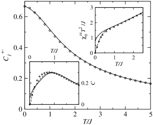
Figure 2: $D=0$ limit: Nearest-neighbor correlation function $C_{1}^{+-}$, longitudinal spin susceptibility $\chi_{0}^{zz}$ (upper inset), and specific heat $C$ (lower inset) for $S=1$, as obtained by the Green-function theory in the thermodynamic limit (solid) and for a finite system with $N=12$ (dashed) in comparison with the ED data for $N=12$ ($\circ$). The Green-function results for $C_{1}^{+-}$ obtained for $N=12$ and $N\to\infty$ agree within the accuracy of drawing.

In Fig. 2 our results for $S=1$ are plotted, where a remarkably good agreement of the Green-function theory for $N=12$ with the ED data is found. This justifies the decouplings (9) and (14) with $\lambda$ calculated by Eq. (32). Considering the specific heat, the temperature of the maximum in the theory, $T_{m}^{C}=0.9J$ for both $N=12$ and $N\to\infty$, only slightly deviates from the ED result $T_{m}^{C}=0.8J$. Note that $T_{m}^{C}$ in the semiclassical approach of Ref. CTV00, agrees with the ED value. Concerning the uniform static susceptibility in the thermodynamic limit, we have (see also Ref. SSI94, ) $\lim_{T\to 0}\chi_{0}^{zz}T^{2}/J=\frac{2}{3}S^{4}$. This low-temperature behavior, $\chi_{0}^{zz}\propto T^{-2}$, qualitatively agrees with the result of the renormalization-group approach of Ref. Kop89, , but quantitatively deviates from the finding $\lim_{T\to 0}\chi_{0}^{zz}T^{2}/J=1.58S^{2}$. Kop89

Finally, let us compare our theory with the Green-function approach of Ref. BZS96, for the $S=1$ antiferromagnetic Heisenberg chain. There, instead of the decoupling (14), the left-hand side is rewritten as $S_{i}^{-}S_{j}^{z}S_{j}^{+}=S_{i}^{-}S_{j}^{+}S_{j}^{z}+S_{i}^{-}S_{j}^{+}$. The first term is decoupled analogous to Eq. (14) as $\alpha\langle S_{i}^{-}S_{j}^{+}\rangle S_{j}^{z}$, whereas the second term yields a contribution to $i\dot{S}_{i}^{z}$. This results in a gap $\Delta$ in $\omega_{q}^{zz}$ at $q=0$ which, for $D=0$, is given by $\Delta=J$. In Ref. BZS96, , $\Delta$ is interpreted as a Haldane gap. As we have verified, $\Delta$ is independent of $S$. However, for $S=\frac{3}{2}$, for example, there is no Haldane gap. That means, the gap $\Delta$ is an artefact of the approach of Ref. BZS96, employing commutation before decoupling. According to our experience (see, e.g., the Green-function theory for the $t-J$ modelWI98 ) such a procedure should be avoided. Furthermore, we argue that the approach of Ref. BZS96, yields $\Delta\neq 0$ for the $S=1$ antiferromagnet also in higher dimensions and for the $S\geqslant 1$ ferromagnetic chain. Concluding, contrary to the reasonings of Ref. BZS96, , the Haldane physics cannot be captured by the second-order Green-function theory.

IV EFFECTS OF SPIN ANISOTROPY

To complete our Green-function scheme for the model (1) with $D>0$ and $J>0$ (hereafter, we set $J=1$), the four parameters $\alpha^{\nu\mu}$ and $\lambda^{\nu\mu}$ have to be determined. In the ground state, for $D>0$ we have the exact results

$$C_{n}^{+-}(0)=S\delta_{n,0};\;\;\;C_{n}^{zz}(0)=S^{2}$$ (33)

so that $C_{n\neq 0}(0)=S^{2}$. By Eq. (5) we get $C_{n}^{+-}(0)=\frac{1}{N}\sum_{q}\frac{M_{q}^{+-}}{2\omega_{q}^{+-}}\text{e}^{iqn}$ and, comparing with Eq. (33),

$$M_{q}^{+-}=2S\omega_{q}^{+-}.$$ (34)

Inserting $M_{q}^{+-}$ and $\omega_{q}^{+-}$ given by Eqs. (3) and (15) to (17) with $\eta(0)=1$ [see Eq. (11)] and comparing the coefficients in Eq. (34) in front of $(1-\cos q)^{n}\;(n=2\text{ and }0\text{ or }1)$, we obtain

$$\alpha^{+-}(0)=1;\;\;\lambda^{+-}(0)=1-\frac{1}{2S}.$$ (35)

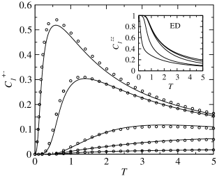
Figure 3: Nearest-neighbor transverse spin correlation functions $C_{1}^{+-}$ for $S=1$ at $D=0.1,1,5,10$, and 25, from top to bottom, showing the Green-function (solid) and ED results ($\circ,\;N=12$). The inset shows the ED data for the nearest-neighbor longitudinal correlation functions $C_{1}^{zz}$ at the same values of D with D increasing from bottom to top, which are used as input to the Green-function theory.

Considering finite temperatures and suggesting $\lim_{T\to\infty}\alpha^{+-}(T)=1$ (see Sec. III), we put $\alpha^{+-}(T)=1$ because of $\alpha^{+-}(0)=1$. Following the reasonings in the $D=0$ limit, for the ratio $Q^{+-}\equiv\lambda^{+-}/\alpha^{+-}$ we assume $Q^{+-}(T)=Q^{+-}(0)$, i.e. $\lambda^{+-}(T)=\lambda^{+-}(0)$. The parameter $\alpha^{zz}(T)$ is calculated from the sum rule (7). Concerning the remaining parameter $\lambda^{zz}$ and the ratio $Q^{zz}\equiv\lambda^{zz}/\alpha^{zz}$, it turns out that $Q^{zz}$ has very different values in the $T\rightarrow 0$ and $T\rightarrow\infty$ limits. Therefore, we adjust $\lambda^{zz}(T)$ to the ED data for $C_{1}^{zz}(T)$ which are depicted, for $S=1$, in the inset of Fig. 3. Thus, we have a closed system of equations for seven quantities ($C_{0}^{\nu\mu},C_{1}^{+-},C_{2}^{\nu\mu},\alpha^{zz},\lambda^{zz}$) to be determined self-consistently as functions of temperature.

As a first test of our approach, in Fig. 3 the NN correlation function $C_{1}^{+-}$ for $S=1$ is plotted, where a very good agreement with the ED results is found. The correlator $C_{0}^{+-}$ (not shown) also agrees very well with the ED data. As can be seen, we have $C_{1}^{+-}<2C_{1}^{zz}$; that is, due to the easy-axis anisotropy the transverse correlations are suppressed as compared with the longitudinal correlations. The maximum in the temperature dependence of $C_{1}^{+-}$ indicates the crossover from Ising-like to Heisenberg-like behavior, where the maximum position increases with increasing $D$.

IV.1 Spin waves

At $T=0$, by Eq. (34) with Eqs. (3) and (33) we obtain the spin-wave spectrum

$$\omega_{q}^{+-}(0)=2S(1-\cos q)+(2S-1)D$$ (36)

with the spin-wave gap $\omega_{0}^{+-}(0)=(2S-1)D$. Let us point out that the dispersion (36) agrees with the result obtained by the RPA and the Anderson-Callen decoupling (see, e.g., Ref. FJK00, ) given by $B_{i}\equiv S_{i}^{+}S_{i}^{z}+S_{i}^{z}S_{i}^{+}=2\langle S^{z}\rangle\left\{1-\frac{1}{2S^{2}}\cdot[S(S+1)-C_{0}^{zz}]\right\}S_{i}^{+}$; putting, at $T=0$, $\langle S^{z}\rangle=S$ and $C_{0}^{zz}=S^{2}$ so that $B_{i}=2S-1$, the spectrum (36) results. In the RPA approach of Ref. FKS02, , where the $D$ term for $S=1$ is treated exactly, we calculate $\chi_{q}^{+-}(\omega)=-2(\omega-\omega_{q})^{-1}$ (correcting a misprint in Eq. (51) of Ref. FKS02, ) with $\omega_{q}$ given by Eq. (36) with $S=1$.

Let us compare Eq. (36) with previous spin-wave theories. The generalized spin-wave theory by Becker Bec72 for $S=1$, which extends the Holstein-Primakoff transformation to two sets of Bose operators treating the single-ion anisotropy exactly, yields $\omega_{0}^{+-}(0)=D$, in agreement with Eq. (36). Contrary, in the ordinary spin-wave theory (with only one Bose operator $a_{i}$), $(S_{i}^{z})^{2}$ with $S_{i}^{z}=S-n_{i}$ and $n_{i}=a_{i}^{+}a_{i}$ is approximated as $(S_{i}^{z})^{2}=S^{2}-2Sn_{i}$ neglecting the $n_{i}^{2}$ term. This yields the wrong result $\omega_{0}^{+-}=2SD$ violating the condition $\omega_{0}^{+-}(S=\frac{1}{2})=0$. Note that such an approach was used to fit the inelastic neutron-scattering data on LaMnO₃ on the basis of an effective spin model with easy-axis single-ion anisotropy. Mou96 From our results we conclude that this fit should be reconsidered by means of an improved theory.

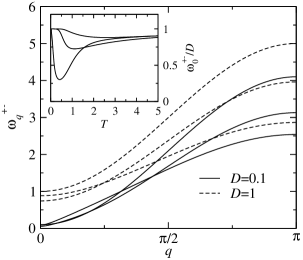
Figure 4: Spin-wave spectrum $\omega_{q}^{+-}$ for $S=1$ at $T=0,1,$ and 5, at $q=\pi$ from top to bottom. The inset shows the spin-wave gap $\omega_{0}^{+-}$ at $D=0.1,1,$ and 5, at $T=1$ from bottom to top.

Figure 5: Inverse correlation length for $S=1$ at $D=0.1,1,5,10$, and 25, from top to bottom (solid), compared with the $D=0$ limit (dashed).

Figure 6: Transverse (a) and longitudinal (b) uniform static spin susceptibility for $S=1$ at $D=1,5,10$, and 25, from left to right, obtained by the ED ($\circ$) for $N=8$ (a) and $N=12$ (b) and by the Green-function theory (solid). In the insets on the left-hand side, for $D=0.1$ the Green-function results for $N\rightarrow\infty$ (solid) and $N=8$ (dashed) are compared with the ED data for $N=8$. In the inset on the right-hand side of (a) the position of the susceptibility maximum $T_{m}^{\chi}$ vs $D$ is depicted.

In Fig. 4 the temperature dependence of the spin-wave spectrum for $S=1$ is shown, where a spin correlation-induced flattening of the shape with increasing temperature is observed. The spin-wave gap as function of temperature exhibits a minimum and approaches the high-temperature limit $\lim_{T\to\infty}\omega_{0}^{+-}(T)=\omega_{0}^{+-}(0)$. In the paraphase ($T>0$) with SRO, well-defined spin waves exist, if their wavelength is much smaller than the correlation length, i.e., if $q\gg(\xi^{zz})^{-1}$. To estimate the validity region of the spin-wave picture, in Fig. 5 the inverse correlation length is plotted. For $D=0$ we get $\lim_{T\to 0}\xi^{zz}T=S^{2}$ (cf. Ref. SSI94, ) which nearly agrees with the result of the renormalization-group approach, Kop89 $\lim_{T\to 0}\xi^{zz}T=1.14S^{2}$. For $D>0$ the low-temperature behavior of $\xi^{zz}$ is quite different. By Eq. (21) we have $\xi^{zz}=\sqrt{2\bar{\alpha}^{zz}/\Delta^{zz}}$ and $(\xi^{zz})^{-2}\chi_{0}^{zz}=C_{1}^{+-}/\bar{\alpha}^{zz}$ with $\bar{\alpha}^{zz}\equiv\alpha^{zz}C_{1}^{+-}$, where the numerical evaluation yields a finite value of $\bar{\alpha}^{zz}$ as $T\to 0$. Because $(\chi_{0}^{zz})^{-1}(0)=0$, $(\xi^{zz})^{-2}$ approaches zero as $T\to 0$ much stronger than $C_{1}^{+-}$ and $(\chi_{0}^{zz})^{-1}$ (compare Fig. 5 with Figs. 3 and 6). Correspondingly, the easy-axis anisotropy drives the paraphase at low temperatures close to long-range order. As can be seen from Fig. 5, the validity region of the spin-wave picture, $q\gg(\xi^{zz})^{-1}$, shrinks with increasing temperature, where predominantly high-energy magnons may be observed.

IV.2 Spin susceptibility

The spin anisotropy results in a qualitatively different temperature dependence of the uniform static susceptibilities $\chi_{0}^{+-}$ and $\chi_{0}^{zz}$, as can be seen from Fig. 6. Note that the ED calculation of $\chi_{0}^{+-}$ requires a small magnetic field in the $x$ direction so that the $S=1$ data can be obtained only for $N=8$.

The transverse susceptibility $\chi_{0}^{+-}$ (Fig. 6a) reveals a maximum at $T_{m}^{\chi}$, where $T_{m}^{\chi}$ increases with D (right inset), in very good agreement with the ED results. For small anisotropies (left inset) a pronounced finite-size effect is observed, where the theory for $N=8$ agrees well with the ED data. The temperature dependence of $\chi_{0}^{+-}$ may be explained as follows. The anisotropy-induced longitudinal SRO (cf. Fig. 5) results in a spin stiffness against the orientation of the transverse spin components along an external field perpendicular to the $z$ direction. Consequently, at zero temperature $\chi_{0}^{+-}(0)=2/D$ decreases with increasing $D$, and at intermediate temperatures $\chi_{0}^{+-}(T)$ exhibits a maximum.

Considering the longitudinal susceptibility $\chi_{0}^{zz}$ (Fig. 6b), it shows qualitatively the same behavior as in the $D=0$ limit; in particular, $\chi_{0}^{zz}$ diverges as $T\to 0$ indicating the ferromagnetic phase transition. For $T\gtrsim T_{0}$ the Curie law $\chi_{0}^{+-}=2\chi_{0}^{zz}=4/3T$ holds approximately, where, e.g., $T_{0}=2.5\;(3)$ for $D=0.1\;(1)$ and $S=1$.

IV.3 Specific heat

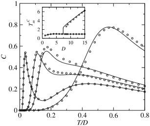
Figure 7: Specific heat $C$ for $S=1$ vs $T/D$ at $D=1,5,7.4$, and 25, from right to left, comparing the Green-function (solid) with the ED ($\circ,\;N=12$) results. The inset shows the positions of the maxima $T_{m}^{C}$ in the temperature dependence of the specific heat as functions of D.

In Figs. 7 to 9 the temperature dependence of the specific heat for the $S=1$ chain is presented. As the main result, the ED on $N=12$ chains with periodic boundary conditions yields two maxima at $T_{m_{1}}^{C}$ and $T_{m_{2}}^{C}$, if $D>D_{0}$ with $D_{0}=7.4$, and only one maximum at $T_{m}^{C}$ for $D<D_{0}$. Let us first consider the specific heat for $D\geqslant 1$ plotted in Fig. 7. The Green-function results for $N\to\infty$, agreeing with those for $N=12$ within the accuracy of drawing, are in a very good agreement with the ED data. Our results for the maximum positions nearly agree with those of Blöte BLO75 obtained by the ED of $N=7$ chains with open boundary conditions and subsequent extrapolations to $N\to\infty$. For example, for $D=1\;(5)$ we get $T_{m}^{C}=0.57\;(0.85)$, as compared with $T_{m}^{C}=0.5\;(1.0)$ in Ref. BLO75, ; for $D=10>D_{0}$ we obtain the maximum temperatures $T_{m_{1}}^{C}=0.85$ and $T_{m_{2}}^{C}=3.93$ which are slightly larger than the values found in Ref. BLO75, , $T_{m_{1}}^{C}=0.79$ and $T_{m_{2}}^{C}=3.77$. At $D=D_{0}$ the specific heat reveals a plateau within a small temperature region, $2.4\lesssim T\lesssim 2.7$ (cf.  Fig. 7). Correspondingly, the dependence on $D$ of the maximum position exhibits a jump at $D_{0}$, as seen in the inset of Fig. 7. For $D>D_{0}$, following the reasonings of Ref. BLO75, the upper maximum at $T_{m_{2}}^{C}$ may be interpreted as Schottky anomaly due to the $D$ term.

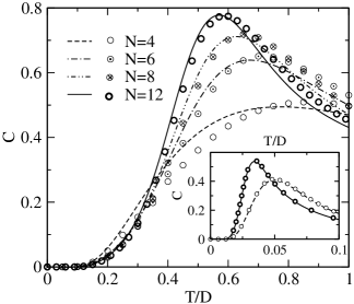
Figure 8: Specific heat for $S=1$ at $D=1$ and $D=25$ (inset: $N=4,12$) and its dependence on the number of spins, where the Green-function results (line styles) are compared with the ED data (circles).

To analyze the finite-size effects on the specific heat for $D\geqslant 1$ and the accuracy of the Green-function approach in dependence on the chain length $N$ and on $D$, in Fig. 8 the specific-heat curves for different values of $N$ with $4\leqslant N\leqslant 12$ and for $D=1$ and $D=25$ (see inset) are plotted. As can be seen, the deviation of the Green-function results from the corresponding ED data decreases with increasing $N$ and $D$. Comparing the curves for $D=1$ and $D=25$, the finite-size effects decrease with increasing $D$. Moreover, they are found to decrease with increasing temperature which is not shown in Fig. 8, where, e.g. for $D=25$, only the low-temperature maximum is depicted (cf. Fig. 7).

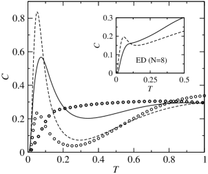
Figure 9: Specific heat for $S=1$ at $D=0.1$ and its dependence on the number of spins, where the ED results for $N=12$ (o) and $N=4$ (o) are compared with the Green-function theory for $N\rightarrow\infty$ (solid) and $N=4$ (dashed). In the inset, the dependence of the specific heat on the periodic (solid) versus open (dashed) boundary conditions in the ED calculations for $N=8$ is demonstrated.

Considering the specific heat at small anisotropies, the detailed analysis of our ED calculations for different chain lengths with periodic versus open boundary conditions reveals considerable finite-size effects, in contrast to the case $D\geqslant 1$ discussed above, and a remarkable dependence of the ED data on the chosen boundary condition. In this paper we prefer to use periodic boundary conditions, since, due to the translational symmetry implying equivalent lattice sites, (i) the finite-size effects are expected to be less pronounced and (ii) ED calculations for larger systems ($N\leqslant 12$) can be performed, as compared with open boundary conditions used by BlöteBLO75 for $N\leqslant 7$. In Fig. 9 we illustrate the finite-size effects and the influence of boundary conditions for $D=0.1$. The ED data for $N=4$ yield a maximum at $T_{m_{1}}^{C}\simeq 0.05$ which vanishes for $N=12$. This may be understood as follows. In finite systems the spin excitations are gapped, even in the $D=0$ limit, where the finite-size gap $\Delta_{N}$ scales as $N^{-\alpha}$ with $\alpha>0$. If $D<\Delta_{N}$, a low-temperature Schottky-type anomaly in the specific heat may appear and vanish for larger $N$ with $D>\Delta_{N}$. Note that both ED curves approach each other at $T\gtrsim 5$. In the Green-function theory for $N=4$ a maximum is also found at the same temperature $T_{m_{1}}^{C}=0.1$, but with a too large height. However, for $N\to\infty$ this maximum is only weakened, but does not disappear. In view of our ED results for $N=12$, this behavior of the specific heat has to be considered as an artefact of the Green-function theory for small anisotropies. As can be seen from the inset of Fig. 9, the use of open boundary conditions favors the appearance of a spurious low-temperature maximum in the specific heat.

In view of our analysis described above, we consider the ED results by Blöte BLO75 on the specific heat of the $S=1$ ferromagnetic chain with $D\lesssim 0.25$ as questionable, in particular, because the extrapolation of the data for small systems with $N\leqslant 7$ and open boundary conditions was performed. Our ED results on the specific heat at small anisotropies qualitatively deviate from the data by Blöte.BLO75 In Ref. BLO75, two maxima were obtained not only for large values of $D$ (see above), but also for $D\lesssim 0.25$, where for $D=0.1$ a low-temperature maximum was found at $T_{m_{1}}^{C}=0.12$. In our ED data at large enough $N$ such a maximum does not appear.

IV.4 Comparison with experiments

Finally, let us compare the results of the Green-function theory with some experiments on Ni complexes KBD74 and derive predictions for quantities not yet measured.

Figure 10: Specific heat $C$ of the Ni complexes NiBr${}_{2}\cdot 2py$ (a) and NiBr${}_{2}\cdot 2pz$ (b), where the Green-function theory (solid) is fit to the experimental data ($\blacklozenge$, Ref. KBD74, ). The insets show the predicted temperature dependences of the transverse magnetic susceptibility $\chi_{m}^{+-}$.

In Fig. 10 the specific heat of the di-bromo Ni complexes NiBr₂L₂ with L=pyrazole ($pz$, N₂C₃H₄) and L=pyridine ($py$, NC₅H₅) is depicted. Those compounds can be considered as weakly antiferromagnetically coupled ferromagnetic chains with a large easy-axis single-ion anisotropy.KBD74 The small values of the Neél temperatures $T_{N}$ indicated in Fig. 10 reflect the pronounced quasi-1D behavior. The anomaly of the specific heat at $T_{N}$ cannot be described by our theory for a purely 1D system. For NiBr${}_{2}\cdot 2py$ (Fig. 10a), this anomaly masks the low-temperature maximum at $T_{m_{1}}^{C}$. At sufficiently high temperatures $T>T_{N}$ the systems exhibit 1D behavior, and the theory may be compared with experiments. For NiBr${}_{2}\cdot 2py\;(2pz)$ the fit to the specific heat data yields $J=0.4$meV (0.48meV) and $D=3$meV (2.7meV) so that $D/J=7.5\;(5.6)$, where the first ratio slightly exceeds $D_{0}/J$. Note that those values nearly agree with the findings of Ref. KBD74, . Using the fit values for $J$ and $D$ we calculate the temperature dependence of the transverse magnetic susceptibility $\chi_{m}^{+-}=4\mu_{B}^{2}N_{A}\chi_{0}^{+-}$ ($N_{A}$ is the Avogadro constant). The results (see insets of Fig. 10) show a maximum of $\chi_{m}^{+-}(T)$ at $T_{m}^{\chi}>T_{N}$, where

$$T_{m}^{\chi}=\left\{\begin{array}[]{lll}5.35\text{K }&;&2py\\ 6.25\text{K }&;&2pz\\ \end{array}\right.,$$ (37)

which should be confirmed experimentally.

Figure 11: Spin-wave spectra $\omega_{q}^{+-}$ for NiBr${}_{2}\cdot 2py$ (solid) and NiBr${}_{2}\cdot 2pz$ (dashed) at $T=5$K and 10K, from top to bottom, and inverse correlation length $(\xi^{zz})^{-1}$ (inset), as predicted by the Green-function theory ($q$ and $\xi^{zz}$ are given in units of the lattice spacing.).

Furthermore, in Fig. 11 we show the spin-wave spectrum and the correlation length (inset) calculated for the $J$ and $D$ values given above. Those results may be verified by neutron scattering experiments on single crystals. As disscussed in Sec. A, spin-waves in the paramagnetic phase may be observed, if $q\gg(\xi^{zz})^{-1}$. For example, at $T=5$K this condition may be fullfilled for NiBr${}_{2}\cdot 2py\;(2pz)$ with $(\xi^{zz})^{-1}=0.47\;(0.16)$. At $T=10$K we have $(\xi^{zz})^{-1}=1.16\;(0.74)$ for the $2py\;(2pz)$ complex, so that only Brillouin-zone boundary magnons in NiBr${}_{2}\cdot 2pz$ may be observable.

V SUMMARY

In this paper we have developed a Green-function theory for $S\geqslant 1$ ferromagnetic Heisenberg chains with an easy-axis on-site anisotropy, where products of three spin operators are approximated in terms of one spin operator. Moreover, we have performed exact diagonalizations of chains with up to $N=12$ sites imposing periodic boundary conditions. To investigate the spin-wave picture in the paramagnetic phase, we have calculated the magnon spectrum and the correlation length. The thermodynamic properties (longitudinal and transverse susceptibilities, specific heat) at arbitrary temperatures were found to be in good agreement with the exact results for finite chains. A detailed analysis of the ED data for the specific heat yields two maxima in the temperature dependence for $D/J>7.4$, whereas for $D/J<7.4$ only one maximum appears. Our results at low ratios $D/J$ contradict those of Ref. BLO75, obtained on smaller chains with open boundary conditions. The Green-function theory was compared with specific heat experiments on di-bromo-pyrazole/pyridine Ni complexes, and predictions for the spin-wave spectrum, the correlation length, and the maximum in the temperature dependence of the transverse magnetic susceptibility were made.

- (1) Quantum Magnetism, Lecture Notes in Physics, Vol. 645, edited by U. Schollwöck, J. Richter, D. J. J. Farnell, and R. F. Bishop (Springer, Berlin, 2004).
- (2) G. Kamieniarz and C. Vanderzande, Phys. Rev. B 35, 3341 (1987); G. M. Wysin and A. R. Bishop, Phys. Rev. B 34, 3377 (1986).
- (3) T. Masuda, A. Zheludev, A. Bush, M. Markina, and A. Vasiliev, Phys. Rev. Lett. 92, 177201 (2004); S. L. Drechsler, J. Málek, J. Richter, A. S. Moskvin, A. A. Gippius, and H. Rosner, Phys. Rev. Lett. 94, 039705 (2005).
- (4) A. P. Ramirez, J. Phys. : Condens. Matter 9, 817 (1997); E. L. Nagaev, Phys. Rep. 346, 387 (2001).
- (5) F. Moussa, M. Hennion, J. Rodriguez-Carvajal, H. Moudden, L. Pinsard, and A. Revcolevschi, Phys. Rev. B 54, 15149 (1996); F. Moussa, M. Hennion, G. Biotteau, J. Rodríguez-Carvajal, L. Pinsard, and A. Revcolevschi, Phys. Rev. B 60, 12299 (1999).
- (6) J. Kondo and K. Yamaji, Prog. Theor. Phys. 47, 807 (1972); K. Yamaji and J. Kondo, Phys. Lett. 45 A, 317 (1973).
- (7) E. Rhodes and S. Scales, Phys. Rev. B 8, 1994 (1973).
- (8) H. Shimahara and S. Takada, J. Phys. Soc. Jpn. 60, 2394 (1991).
- (9) F. Suzuki, N. Shibata, and C. Ishii, J. Phys. Soc. Jpn. 63, 1539 (1994).
- (10) S. Winterfeldt and D. Ihle, Phys. Rev. B 56, 5535 (1997); Phys. Rev. B 59, 6010 (1999).
- (11) D. Ihle, C. Schindelin, and H. Fehske, Phys. Rev. B 64, 054419 (2001).
- (12) I. Junger, D. Ihle, J. Richter, and A. Klümper, Phys. Rev. B 70, 104419 (2004).
- (13) D. Schmalfuß, J. Richter, and D. Ihle, Phys. Rev. B 70, 184412 (2004).
- (14) O. Golinelli, Th. Jolicoeur, and R. Lacaze, Phys. Rev. B 46, 10854 (1992).
- (15) N. A. Potapkov, Theor. Mat. Fiz. 8, 381 (1971).
- (16) P. Fröbrich, P. J. Jensen, and P. J. Kuntz, Eur. Phys. J. B13, 477 (2000).
- (17) P. Fröbrich, P. J. Kuntz, and M. Saber, Ann. Phys. (Leipzig) 11, 387 (2002).
- (18) H. W. J. Blöte, Physica 79B, 427 (1975).
- (19) F. W. Klaaijsen, H. W. J. Blöte, and Z. Dokoupil, Soild State Comm. 14, 607 (1974).
- (20) K. Elk and W. Gasser, Die Methode der Greenschen Funktionen in der Festkörperphysik (Akademie-Verlag, Berlin, 1979); W. Nolting, Quantentheorie des Magnetismus, vol. 2 (B. G. Teubner, Stuttgart, 1986).
- (21) P. J. Jensen, and F. Aguilera-Granja, Phys. Lett. A 269, 158 (2000).
- (22) A. Cuccoli, V. Tognetti, P. Verrucchi, and R. Vaia, Phys. Rev. B 62, 57 (2000).
- (23) P. Kopietz, Phys. Rev. B 40, 5194 (1989).
- (24) S. Q. Bao, H. Zhao, J. L. Shen, and G. Z. Yang, Phys. Rev. B 53, 735 (1996).
- (25) S. Winterfeldt and D. Ihle, Phys. Rev. B 58, 9402 (1998).
- (26) K. Becker, Int. J. Magn. 3, 239 (1972).