Single Molecule Chemical Reaction: Kramers Approach Revisited

Abstract

Single molecule chemical reactions yield new insight into fluctuation phenomena which are obscured in measurement of ensemble of molecules. Kramers escape problem is investigated here in a framework suitable for single molecule reactions. In particular we obtain distributions of escape times in simple limiting cases, rather than their mean, and investigate their sensitivity on initial conditions. Rich physical behaviors are observed: sub-Poissonian statistics when the dynamics is only slightly deviating from Newtonian, super-Poissonian behavior when diffusion is dominating, and Poissonian behavior when Kramers original conditions hold. By varying initial conditions escape time distributions can follow a (usual) exponential or a $\tau^{-3/2}$ decay, due to regular diffusion. We briefly address experimental results which yield the $\tau^{-3/2}$ behavior (with cutoffs) and propose that this behavior is universal.

Chemical reaction of a single molecule evolving between two states $A\rightleftharpoons B$ or of two species $A+B\rightleftharpoons AB$ is now followed in many laboratories using single molecule spectroscopy techniques Xie (2002); Barkai et al. (2004); Lu et al. (1998); Deniz et al. (2000); Rhoades et al. (2003, 2004); Flomenbom et al. (2005). Such experiments yield detailed statistical information on chemical conformational changes, and simple chemical processes in condensed phase environments, for example the distribution of occupation times of states A and B in the process $A\rightleftharpoons B$. Such information is impossible to obtain when measurements are made on many molecules, since the ensemble averaging wipes out the detailed information found on the single molecule level. For ensemble of molecules, usually simple reactions are assumed to follow a rate process.

For ensemble of molecules undergoing a chemical reaction, classical concepts like reaction coordinate, and rate equations, work well in many cases. In particular Kramers model Kramers (1940); Hänggi et al. (1990) for activation over a barrier, is a fundamental tool for modeling chemical reactions in condensed phase environments. In this manuscript we analyze Kramers problem, in a framework of single molecules. We first discuss Kramers original approach, and its limitations in the single molecule domain.

Kramers describes a chemical reaction in terms of a reaction coordinate $x(t)$. The complicated interaction of the chemical species with their environment is replaced with a stochastic one dimensional approach. The coordinate $x(t)$ evolves in a deterministic force field $V(x)$, and is also coupled to a thermal heat bath. The reaction coordinate is supposed to escape a metastable state. The inverse of the average time of escape $\left\langle\tau\right\rangle$, from the bottom of the well, serves as an estimate on the ensemble averaged reaction rate. Two important regimes of Kramers problem are the underdamped and overdamped limits. Many refinements, non-trivial results and generalizations of Kramers problem are known, e.g. Kramers turn over behavior, quantum effects, and non-Markovian generalizations (e.g., Büttiker et al. (1983); Mel’nikov and Meshkov (1986); Drozdov and Brey (1999); see Hänggi et al. (1990) for a review). Experimental validation of the theory is also obtained McCann et al. (1999).

At least three aspects of Kramers problem must be revised in the context of single molecule chemical reaction. The most obvious one is that now we must consider the distribution of occupation times in a chemical state, and not limit the theory to averaged escape rates. Previous work considered temporal dependence of the rate Chen and Nash (2004); Bao and Jia (2004) until it reaches an equilibrium value in a single escape (transition) event, or the transient behavior after the particle injection close to the bottom of the well Shneidman (1997). The idea of fluctuating rates in multiple transitions, in the context of single molecule experiments has been scrutinized and used in, e.g., Wang and Wolynes (1995); Chernyak et al. (1999); Xie (2002); Brown (2003). A second issue is the sensitivity of single molecule chemical reactions to initial conditions. Consider the ongoing chemical reaction $A\rightleftharpoons B$. For example using fluorescence resonance energy transfer (FRET) methods, one may follow the closing (state A) and opening (state B) of a large molecule Weiss (1999); Selvin (2000); Deniz et al. (2000); Rhoades et al. (2003, 2004). The experimental data then yields the string of occupation times $\{\tau_{A}^{1},\tau_{B}^{2},\tau_{A}^{3},....\}$. Following Kramers assume that such events are described by a reaction coordinate, which goes over a single barrier, to cross from state $A\rightarrow B$ and vice versa. Also we assume that a measurement may distinguish between state $A$ and state $B$, as is shown in many experiments. In terms of the reaction coordinate this means that when $x(t)<x_{b}$ the system is in the state $A$, otherwise it is in the state $B$ and $x_{b}$ is the boundary (usually and conveniently assumed to be at the top of the potential barrier). Then immediately after the transition event from say $A\rightarrow B$, the reaction coordinate is in close vicinity to $x_{b}$. Thus a short time after the transition from state $A\rightarrow B$ there is an increased likelihood for a back transition $B\rightarrow A$. This possibility is expected to yield bunching of chemical activity on the time axis, i.e. to intermittency where strong activity is observed for some period of time followed by periods of lesser activity. Of course to observe such effects the resolution time in the experiments must be short compared to relaxation times of the dynamics. A third important point is that in single molecule experiments, an additional length scale $\lambda$ is introduced into the problem. For example the radius of the laser illumination field, or the Förster length scale in FRET experiments Selvin (2000); Deniz et al. (2000). Roughly, in the reaction $A\rightleftharpoons B$, a fluorescence signal is recorded if an acceptor and donor are within a range of Förster radius from each other (state A) while otherwise the signal is zero (state B). In terms of the reaction coordinate this implies that when $x(t)<\lambda$ the system is in the state $A$ otherwise it is in the state $B$. The point to notice is that in principle $\lambda$ can be anywhere along the reaction coordinate. In particular the classical approach of an escape from a bottom of the well over a maximum in the potential field is not expected to be general.

Hence we investigate Kramers escape problem, obtaining distribution of escape times. With initial conditions both in vicinity of the escape point and far from it. We classify the deviations from exponential behaviors, and show that in many cases rate concept is not valid. In particular we classify a turnover behavior from power law behavior to exponential, and show that the power law behavior is general.

Model 1 We consider a classical particle undergoing underdamped diffusion in a harmonic potential well. As well known the relevant coordinate for underdamped motion is the action $I$. The probability density function (PDF) P of finding the particle with action $I$ obeys

$$\frac{\partial P}{\partial t}=\gamma\frac{\partial}{\partial I}\left(IP+\frac{2\pi k_{B}T}{\omega}I\frac{\partial P}{\partial I}\right)$$ (1)

where $\omega$ is the harmonic frequency, $E$ is the particle energy, $k_{B}T$ is the thermal energy, and $\gamma$ is the damping coefficient; $\gamma\ll\omega$ (see Fig.

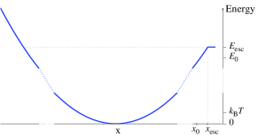
Figure 1: Escape from a metastable well. In the underdamped case, the relevant coordinate is the action $I$, which is related to the energy $E$ of the particle by $I=2\pi E/\omega$. In the overdamped case, the relevant coordinate is position x in real space.

1; $I=2\pi E/\omega$ for constant $\omega$). In what follows we use dimensionless time $\tau=\gamma t$ and action $\mathcal{I}=I\omega/2\pi k_{B}T$. Let $\phi(\tau)$ be the PDF of escape times from $\mathcal{I}_{0}$ to $\mathcal{I}_{esc}>\mathcal{I}_{0}$. Mathematically we use absorbing boundary conditions at $\mathcal{I}_{esc}$, so that $\phi(\tau)$ is the first passage time distribution (FPTD) from $\mathcal{I}_{0}$ to $\mathcal{I}_{esc}$. We obtained the Laplace $\tau\rightarrow u$ transform of $\phi(\tau)$, using known solution to Kummer’s equation Abramowitz and Stegun (1972); Siegert (1951). We find

$$\hat{\phi}(u)=\frac{{}_{1}F_{1}(u;1;\mathcal{I}_{0})}{{}_{1}F_{1}(u;1;\mathcal{I}_{esc})}$$ (2)

where ${}_{1}F_{1}(a;b;c)$ is the regular confluent hypergeometric function. Since ${}_{1}F_{1}(0;b;c)=1$ the function $\phi(\tau)$ is normalized to 1. We note that a second presentation of the solution in terms of an infinite sum of exponentially decaying modes is possible, in time domain. However, as we shall show now for an important parameter regime, one cannot replace such standard eigenfunction solutions with a summation over a finite number of modes consisting of a few exponential functions, rather the solution exhibits a power law behavior.

To quantify deviations from exponential statistics, we use the parameter

$$Q=\frac{\sigma^{2}}{\left\langle\tau\right\rangle^{2}}-1,$$

where $\langle\tau\rangle$ is the average escape time and $\sigma^{2}=\left\langle\tau^{2}\right\rangle-\left\langle\tau\right\rangle^{2}$ is its variance. If we have Poissonian behavior consistent with a rate equation approach, then $Q=0$. When the dynamics is Newtonian (i.e. diffusion is weak) the PDF of escape time is narrow, leading to $Q<0$, a sub-Poissonian behavior. On the contrary, if the PDF of escape times is wide spread, there is a super-Poissonian behavior and $Q>0$. Using the small $u$ expansion of the exact solution, we find

$$\left\langle\tau\right\rangle=A(\mathcal{I}_{esc})-A(\mathcal{I}_{0})$$ (3)

and

$$\sigma^{2}=A^{2}(\mathcal{I}_{esc})-A^{2}(\mathcal{I}_{0})-2[B(\mathcal{I}_{esc})-B(\mathcal{I}_{0})]$$ (4)

with

$$\begin{array}[]{ccc}A(z)={\displaystyle\sum_{n=1}^{\infty}\frac{z^{n}}{n\,n!}}&\textrm{and}&B(z)={\displaystyle\sum_{n=2}^{\infty}\frac{z^{n}\sum_{j=1}^{n-1}1/j}{n\,n!}}\end{array}.$$ (5)

In Fig.

Figure 2: $Q+1$ as a function of $r=\mathcal{I}_{0}/\mathcal{I}_{esc}$. Full line is the asymptotic line for small $\mathcal{I}_{esc}$, given by $(1+r)/(2(1-r))$. Dashed line is for $\mathcal{I}_{esc}=1$ and dot-dashed line is for $\mathcal{I}_{esc}=10$. Notice the logarithmic scale. Two generic behaviors are observed: (i) if $\mathcal{I}_{0}\leq 1$, a smooth transition from sub-Poissonian to super Poissonian behavior is observed (ii) if $\mathcal{I}_{0}>1$, a Poissonian behavior is found until $\mathcal{I}_{0}\simeq\mathcal{I}_{esc\,}$ and then a sharp transition from Poissonian to super-Poissonian behavior is observed.

2 we plot $Q+1$ versus $\mathcal{I}_{0}$ for three cases where $\mathcal{I}_{esc}<1$ (escape over a shallow barrier), $\mathcal{I}_{esc}=1$ and $\mathcal{I}_{esc}>1$ (escape over a large barrier). As $\mathcal{I}_{0}\rightarrow\mathcal{I}_{esc}$, namely the case when the chemical reaction starts close to the escaping zone, we observe $Q\rightarrow\infty$, i.e. strong super-Poissonian behavior. For $\mathcal{I}_{esc}\leq 1$ we do not expect, and indeed do not find an exponential behavior, since the barrier is not high. Here, depending on initial position, either sub- or super-Poissonian behavior is generally observed. As $\mathcal{I}_{0}$ becomes closer to $\mathcal{I}_{esc}$, diffusion in Eq. (1) becomes more dominant than the deterministic drift, and hence $Q$ grows. Conversely, when $\mathcal{I}_{0}\ll\mathcal{I}_{esc}$ and $\mathcal{I}_{esc}\leq 1$ drift becomes more important, leading to negative $Q$. However, diffusion can never be neglected as it is the only mechanism leading to an eventual escape from the well. Note that always $Q\geq-1/2$ and the absolute minimum of $Q=-1$ is unachievable in this model. For $\mathcal{I}_{esc}>1$ and $\mathcal{I}_{0}$ sufficiently below $\mathcal{I}_{esc}$, we have exponential behavior and $Q\simeq 0$. The latter case corresponds to Kramers’ original treatment of escape from a deep metastable state.

We now consider $\phi(\tau)$. In Laplace space and in the limit $u\gg\max\{1,1/\mathcal{I}_{0}\}$ we use Abramowitz and Stegun (1972) to reduce Eq. (2) to

$$\hat{\phi}(u)\sim\left(\frac{\mathcal{I}_{esc}}{\mathcal{I}_{0}}\right)^{1/4}e^{(\mathcal{I}_{0}-\mathcal{I}_{esc})/2}e^{-2\sqrt{u}(\sqrt{\mathcal{I}_{esc}}-\sqrt{\mathcal{I}_{0}})}.$$ (6)

The important thing to notice is the non-analytical behavior of this asymptotic solution, namely the term of the form $e^{-\sqrt{u}}$. This term is an indication for power law behavior (with some cutoffs) since if $\hat{\phi}(u)=e^{-\sqrt{u}}$ for all $u$ then $\phi(\tau)\sim\tau^{-3/2}$ for large $\tau$ (e.g., Feller (1966)). To find $\tau$ for which $\phi(\tau)\sim\tau^{-3/2}$ we have to demand the validity of Eq. (6) for small $\sqrt{u}(\sqrt{\mathcal{I}_{esc}}-\sqrt{\mathcal{I}_{0}})$, while $u$ is large. This yields

$$\left(\sqrt{\mathcal{I}_{esc}}-\sqrt{\mathcal{I}_{0}}\right)^{2}\ll\tau\ll\min\{1,\mathcal{I}_{0}\}$$ (7)

so that the reaction should start in the vicinity of the escaping point. This behavior is demonstrated in Fig.

Figure 3: Distribution of escape times $\phi(\tau)$ in the underdamped case. At early and intermediate times $\phi(\tau)$ is governed by Eq. (8), which exhibits a power law decay $\tau^{-3/2}$ at intermediate times (thin line), if the initial condition $\mathcal{I}_{0}$ is close to the escape condition $\mathcal{I}_{esc}$. At later times, there is an exponential decay with rate given by Kramers rate.

3.

When $\tau\rightarrow 0$ we find $\phi(\tau)\rightarrow 0$, a non-exponential behavior. This behavior is due to the fact that it takes the particle a certain amount of time to reach the boundary. More quantitatively, for short times Eq. (6) is always a good approximation for $\hat{\phi}(u)$, leading to

$$\phi(\tau) \sim \left(\frac{\mathcal{I}_{esc}}{\mathcal{I}_{0}}\right)^{1/4}e^{(\mathcal{I}_{0}-\mathcal{I}_{esc})/2}(\sqrt{\mathcal{I}_{esc}}-\sqrt{\mathcal{I}_{0}})$$ (8)

$$\times \frac{\exp[-(\sqrt{\mathcal{I}_{esc}}-\sqrt{\mathcal{I}_{0}})^{2}/\tau]}{\sqrt{\pi}\tau^{3/2}}.$$

Model 2 We turn now to the other limit of particle diffusion - namely to the overdamped limit, and demonstrate the deviation from Poissonian behavior. The relevant coordinate here is the spatial coordinate x. Restricting ourselves to one spatial dimension, the following equation is then obtained:

$$\frac{\partial P(x,t)}{\partial t}=(m\gamma)^{-1}\left[\frac{\partial}{\partial x}U^{\prime}(x)+k_{B}T\frac{\partial^{2}}{\partial x^{2}}\right]P(x,t),$$ (9)

where m is the particle mass and $F(x)=-U^{\prime}(x)$ is the deterministic part of the force, due to potential field. We consider two cases, when $U(x)=\pm m\omega^{2}x^{2}/2$ near the escape point, i.e., parabolic and inverted parabolic potential, with $\omega\ll\gamma$. We define dimensionless time $\tau=t/\theta$ and position $y=x/l$, where $\theta=\gamma\omega^{-2}$ and $l=\sqrt{k_{B}T/\left(m\omega^{2}\right)}$.

Parabolic potential. We are interested in the FPTD from initial position $y_{0}$ to $y_{esc}$. This function is known in Laplace space and is given by (e.g., Siegert (1951))

$$\hat{\phi}(u)=\frac{D_{-u}(-y_{0}s)e^{y_{0}^{2}/4}}{D_{-u}(-y_{esc}s)e^{y_{esc}^{2}/4}}=\frac{H_{-u}(-y_{0}s/\sqrt{2})}{H_{-u}(-y_{esc}s/\sqrt{2})},$$ (10)

where $D_{\lambda}(z)$ is the parabolic cylinder, or Weber function, $H_{-u}(z)$ is the generalization of Hermite polynomials used in mathematica and $s=\textrm{sign}(y_{esc}-y_{0})$. The PDF $\phi(\tau)$ is normalized to 1. Using various formulas from Abramowitz and Stegun (1972) we can simplify Eq. (10) for large $u\gg\max\{y_{esc}^{2},y_{0}^{2}\}$:

$$\hat{\phi}(u)\sim\exp\left[\frac{y_{0}^{2}-y_{esc}^{2}}{4}\right]e^{-\sqrt{u}|y_{esc}-y_{0}|},$$

exhibiting a non-analytical behavior of the $e^{-\sqrt{u}}$ type similar to the previous example. In order to have the $\phi(\tau)\propto\tau^{-3/2}$ scaling we thus have to demand the validity of this approximation for small $\sqrt{u}|y_{esc}-y_{0}|<1$. Together with the condition $u\gg\max\{y_{esc}^{2},y_{0}^{2}\}$ it leads to

$$\left(y_{esc}-y_{0}\right)^{2}\ll\tau\ll\frac{1}{\max\{y_{esc}^{2},y_{0}^{2}\}}.$$ (11)

As we are interested in the escape over the barrier, we have either $y_{0}<y_{esc}$ if $y_{esc}>0$, or $y_{0}>y_{esc}$ if $y_{esc}<0$. In a deep well (low $T$), if $|y_{0}|\ll|y_{esc}|$ then $\phi(\tau)$ will be nearly exponential, similar to Model 1. If the well is not deep, or $y_{0}$ and $y_{esc}$ are close, $Q$ shows a super Poissonian behavior. Noticeably negative $Q$ is only possible if the initial position of the particle is on the other side of the well from the escape point, and high above it in energy (when $y_{0}/y_{esc}$ becomes very negative).

Inverted parabolic potential. The FPTD is now given by

$$\hat{\phi}(u)={\displaystyle\frac{D_{-1-u}(-y_{0}s)}{D_{-1-u}(-y_{esc}s)}\exp\left[\frac{y_{esc}^{2}-y_{0}^{2}}{4}\right]}$$ (12)

The normalization is

$$\hat{\phi}(0)=\frac{1+\textrm{erf}(y_{0}s/\sqrt{2})}{1+\textrm{erf}(y_{esc}s/\sqrt{2})}<1.$$

The normalization is less than 1 in this case because some particles will escape in the direction of $-s\infty$, where the potential drops unbounded. Of course, if the particles are not allowed to escape to infinity, so that the only exit is through $y_{esc}$ then the normalization should be 1. However, the above formulae serve as a good approximation for a deep well, if we consider the behavior around the parabolically shaped escape barrier at sufficiently short times. Similar to the previous section, for  $u\gg\max\{1,y_{esc}^{2},y_{0}^{2}\}$

$$\hat{\phi}(u)\sim\exp\left[\frac{y_{esc}^{2}-y_{0}^{2}}{4}\right]e^{-\sqrt{u}|y_{esc}-y_{0}|}$$

and the condition for observing $\tau^{-3/2}$ scaling is

$$\left(y_{esc}-y_{0}\right)^{2}\ll\tau\ll\frac{1}{\max\{1,y_{esc}^{2},y_{0}^{2}\}}.$$

In this Letter, we demonstrated non-Poisson statistics of escape from a potential well, which contradicts reaction rate approach used for ensemble (bulk) dynamics. Both sub- and super-Poisson statistics were observed, indicated by the sign of the $Q$ parameter. For small travel distances, and for a shallow well in the overdamped case, scaling $\phi\propto\tau^{-3/2}$ is dominant and gives rise to a strong super-Poissonian statistics (cf. Fig. 2). The $\tau^{-3/2}$ behavior is a result of diffusion processes Redner (2001). The occurrence of such a behavior is easily understood if one realizes that in many cases a Fokker-Planck equation with variable coefficients (e.g., Eq. (1)) can locally be approximated by an equation with constant coefficients, i.e., by advection-diffusion equation. As travel distance increases, characteristic time grows and drift term can compete with diffusion, allowing for Poissonian and sub-Poissonian behavior. In the underdamped case sub-Poissonian behavior is found in many cases (see Fig. 2), in the overdamped case we may observe sub-Poissonian behavior only under special conditions. As is well known, near-exponential $\phi(\tau)$ is obtained for a deep well if initial energy is sufficiently below the escape energy.

Finally let us compare our model results to experiments on single molecules and to other models. Blinking nanocrystals exhibit a behavior of occupation times of on and off times close to $\tau^{-3/2}$ with cutoffs Brokmann et al. (2003); Kuno et al. (2003); Shimizu et al. (2001). The blinking is believed to describe charging of a single nanocrystal (charged NC can be off). Shimizu et al. Shimizu et al. (2001) briefly suggested a diffusion in energy space to describe such behavior, however did not consider the effect of dissipation and temperature which are always present in case of diffusion in energy space. Recent experiments on diffusing beads that come in and out of focus of a laser field, also exhibit the $\tau^{-3/2}$ behavior Zumofen et al. (2004). Occupation times in single molecule Raman experiments are described also by $\tau^{-3/2}$ behavior Bizzarri and Cannistraro (2005). Dynamics of single ion channels sometimes exhibit the $\tau^{-3/2}$ Nadler and Stein (1991); Goychuk and Hänggi (2002). Goychuk and Hänggi Goychuk and Hänggi (2002) suggested a model based on a reaction where space is divided into two: a zone with free diffusion (which yields the $3/2$ law) and a zone where the reaction coordinate is climbing over a potential field. While all these systems and models are very different, they all exhibit a universal tendency for a $\tau^{-3/2}$ and in several cases an exponential cutoff is observed. Thus the turn over behavior we found, from a power law behavior, to an exponential behavior, will be a useful concept for the single molecule domain. Further we do not expect this behavior to be limited to Kramers problem, since diffusion is expected to control short time dynamics of many reactions.