Gap-Townes solitons and localized excitations in low dimensional Bose-Einstein condensates in optical lattices

Abstract

We discuss localized ground states of Bose-Einstein condensates in optical lattices with attractive and repulsive three-body interactions in the framework of a quintic nonlinear Schrödinger equation which extends the Gross-Pitaevskii equation to the one dimensional case. We use both a variational method and a self-consistent approach to show the existence of unstable localized excitations which are similar to Townes solitons of the cubic nonlinear Schrödinger equation in two dimensions. These solutions are shown to be located in the forbidden zones of the band structure, very close to the band edges, separating decaying states from stable localized ones (gap-solitons) fully characterizing their delocalizing transition. In this context usual gap solitons appear as a mechanism for arresting collapse in low dimensional BEC in optical lattices with attractive real three-body interaction. The influence of the imaginary part of the three-body interaction, leading to dissipative effects on gap solitons and the effect of atoms feeding from the thermal cloud are also discussed. These results may be of interest for both BEC in atomic chip and Tonks-Girardeau gas in optical lattices.

I Introduction

Bose-Einstein condensates (BEC) in periodic potentials are presently receiving a great deal of theoretical and experimental interest due to the possibility to explore a whole class of phenomena ranging from Bloch oscillations And ; Cris , Landau-Zener tunneling Wu and solitons Eier to quantum phase transitions of the Mott insulator type Gren . In the mean field approximation these systems are described by the Gross-Pitaevskii equation (GPE) which is a cubic nonlinear Schrödinger (NLS) equation with periodic potential in which the cubic nonlinearity models the two-body interatomic interactions appropriate for dilute gases. The presence of the optical lattice (OL) allows interesting localization phenomena such as the formation of gap-solitons, i.e. localized states with energies comprised in the gaps of the band structure of the underlying linear periodic problem, both for attractive and repulsive interactions Baiz ; Ostr . This is quite remarkable because it is known that for two (2D) and three dimensional (3D) NLS, in absence of periodic potential, soliton solutions do not exist and for attractive interactions the phenomenon of collapse in finite time appears. In this last case only one localized solution is possible, the so called Townes soliton, existing for a single value of the norm (number of atoms). This solution however is unstable against norm variations i.e. it collapses in a finite time for norms above the critical value and decays into the uniform background for norms below the critical value. The presence of the OL allows to expand the range of existence of localized solutions from a single value to a whole interval of norms below which the delocalizing transition occurs and above which collapse takes place.

A description based on the GPE with cubic nonlinearity, however, is adequate only at low densities. For higher densities the three-body interactions start to play a role and a description based on two-body interactions is no longer sufficient. Akhmediev ; Zhang ; AGTF ; GFTA . To this regard we recall that condensate densities limited by three-body inelastic collisions ketterle have indeed been achieved. In these regime a more accurate treatment of the mean-field energetics of a dense condensate will need to account for both two- and three-body elastic collisions.

The contribution of the three-body interactions can be enhanced by detuning to zero the cubic two body term by means of Feschbach resonances ketterle , this leading to a periodic NLS equation with quintic nonlinearity. For appropriate values of density and scattering lengths, however, the three-body collisions could largely dominate the two-particle contributions even in a very dilute regime. This occurs when the so called Efimov effect efimov becomes possible i.e. when the two-body scattering length becomes much larger than the effective two body interaction radius (this usually occurring near a two-body resonance). In this case a very large number of three-body bound states can be formed in the system and the contribution of the three-body elastic collisions (cubic in the density) to the energy may largely overcome the one arising from the two-body terms (quadratic in the density). In this situation the condensate appear extremely dilute with respect to the two-body collisions but somewhat dense with respect to the three-body collisions bulgac .

Theoretical estimates of the three-body coefficient were given in Bed ; Braat ; Jack ; Koh . This term can be modeled by a quintic nonlinearity in the GPE which for rubidium atoms is expected to be attractive Zhang . The different types of instabilities induced by the quintic term may lead to interesting dynamical phenomena in 1D BEC similar to Bose-Novae effect observed in multidimensional case. On the other hand, the presence of these instabilities restricts the possibility of BEC manipulations in atomic waveguides Zhang ; AGTF . The optical lattice, however, can suppress or delay some of these instabilities opening the possibility for new types of localized excitations.

The 1D quintic NLS is also used to describe a Bose gas with hard-core interactions in the Tonks-Girardeau regime. Recent works have shown that this approach describes well the ground state properties, the collective oscillations in a parabolic trap Minguzzi and the dynamics of shock waves and dark solitons in the gas Damski ; Kevr . On the other hand, interference phenomena generated with small number of atoms ($N=10$) were shown to be not well accounted by the quintic NLS (the interference patterns obtained from this equation are much more pronounced than the experimental ones) Gir00 . For larger number of atoms and for weak density modulations, however, the description of the nonlinear excitations in the Tonks-Girardeau regime by means of a quintic NLS equation is expected to be valid.

The aim of the present paper is to study localized states of the quintic nonlinear Schrödinger equation with periodic potential for both attractive and repulsive interactions. To this regard we use a variational method, a self-consistent approach and direct numerical integrations, to show that the presence of the optical lattice allows to stabilize solitons of the attractive quintic 1D NLS against collapse or decay. In the case of repulsive interactions the optical lattice is found to be crucial for the existence of stable bright matter waves. The existence of localized excitations in this system is shown to be associated to the existence of unstable localized solutions similar to the Townes soliton of the cubic 2D NLS equation (we refer to them as gap-Townes solitons). These unstable solutions are found to be located in the forbidden zones of the band structure, very close to band edges and separate decaying states from stable gap-solitons. The existence curve of these solutions characterizes the critical threshold for the occurrence of the delocalizing transition and the existence of gap solitons appears to be a mechanism for arresting collapse in 1D BEC in OL with three-body interactions. We also investigate dissipative effects on gap solitons induced by the imaginary part of the three-body interactions. We show that when the imaginary part of this interaction is small compared to the real part, localized states exist for very long times and their behavior is qualitatively similar to the one of the undamped case. For moderate and large damping, however, all localized states in the band gap decay into the Bloch state at the band edge. We find remarkable that even in this case a reminiscence of the existence of gap-Townes solitons survives in focusing-defocusing cycles observed when the number of atoms is close to the critical value for their existence. We also find that these localized states can be stabilized into breather-like excitations by a linear amplification term modeling the feeding of atoms in the condensate from the thermal cloud in the presence of nonlinear damping.

We remark that in absence of periodic potential the quintic 1D NLS equation has a behavior similar to the 2D NLS equation with cubic nonlinearity. The interplay between dimensionality and nonlinearity has indeed been used in the past to investigate collapse in lower dimensional NLS, the critical condition being $D(n-1)-4=0$ where $n$ the order of the nonlinearity in the equation and $D$ is its dimensionality Berge . From this point of view the quintic NLS can be viewed as a 1D model for the 2D GP with cubic mean field nonlinearity and we expect that the results discussed in this paper will apply also to this case.

The paper is organized as follows. In Section II we introduce the 1D model and discuss the range of applicability to different physical situations. In Section III we study the quintic 1D NLS equation with attractive interactions both in absence and in presence of a periodic potential. The effectiveness of the optical lattice to stabilize localized states of the GPE in presence of two-body and three-body interactions is investigated by means of a variational analysis and by direct numerical simulations. We use a self-consistent method to investigate gap solitons and band structures. The existence of gap-Townes solitons is shown in Section IV and the role of usual gap solitons in arresting collapse is discussed. In Section V we investigate the case of repulsive interactions by means of variational analysis, self-consistent method and numerical simulations. The existence of unstable Townes soliton with energies above the band edges and their role in the delocalizing transition is also investigated. In Section VI the dissipative effects introduced by an imaginary part of the three-body interaction on gap solitons are studied both by a modified variational analysis and by direct numerical simulations. The effects of atoms feeding from the thermal cloud are also considered. Finally, in the last section, the main results of the paper are briefly discussed and summarized.

II The model

Let us consider a BEC with two and three-body interactions immersed in an optical lattice and an highly elongated harmonic trap. In the mean field approximation the system is described by the following 3D GPE AGTF

$$i\hbar u_{t} = -\frac{\hbar^{2}}{2m}\nabla^{2}u+[\frac{m}{2}(\omega_{\perp}^{2}\rho^{2}+\omega_{x}^{2}x^{2})+V_{opt}(x)]u$$ (1)

$$+\,g_{1}|u|^{2}u+g_{2}|u|^{4}u,$$

with $\rho$ denoting the radial distance, $g_{1},g_{2}$ the nonlinear coefficients corresponding to the two and three-body interactions, respectively, $\omega_{\perp},\omega_{x}$ the radial and longitudinal frequencies of the anisotropic trap ($\omega_{\perp}\gg\omega_{x}$) and $V_{opt}(x)=V_{0}\sin^{2}(kx)$ the optical lattice applied only in the longitudinal direction. The coupling constant of the two body interaction is related to the s-wave scattering length $a_{s}$ and to the mass $m$ of the atoms by the usual relation $g_{1}=4\pi\hbar^{2}a_{s}/m$. In view of the strong anisotropy of the trap we can average the three dimensional interaction over the radial density profile to reduce the problem to an effective one dimensional one. More precisely, we consider solutions of the form $u(r,t)=\phi_{0}(\rho)\psi(x,t)$ where $\phi_{0}=\sqrt{\frac{1}{\pi a_{\perp}^{2}}}\exp(-\frac{\rho^{2}}{2a_{\perp}^{2}})$ is the ground state of the radial linear equation

$$-\frac{\hbar^{2}}{2m}\nabla_{\rho}^{2}\phi_{0}+\frac{m}{2}\omega_{\perp}^{2}\rho^{2}\phi_{0}=\hbar\omega_{\perp}\phi_{0}.$$ (2)

Multiplying both sides of the GPE by $\phi_{0}$ and integrating over the transverse variable, we obtain the following quasi 1D-GP equation Zhang

$$i\hbar\psi_{t}=-\frac{\hbar^{2}}{2m}\psi_{xx}+(\frac{m}{2}\omega_{x}^{2}x^{2}+V_{0}\sin^{2}(kx))\psi+$$

$$\frac{g_{1}}{2\pi a_{\perp}^{2}}|\psi|^{2}\psi+\frac{g_{2}}{3\pi^{2}a_{\perp}^{4}}|\psi|^{4}\psi.$$ (3)

For a discussion on the limits of applicability of this 1D reduction see Brazh . Introducing the dimensionless variables

$$t=t\nu,x=kx,\;\;\nu=\frac{E_{R}}{\hbar},\;\;\alpha=\frac{\omega_{x}^{2}}{4\nu^{2}},$$ (4)

we reduce Eq. 3 to the following normalized 1D GPE equation with cubic and quintic nonlinearities

$$i\psi_{t}=-\psi_{xx}+g|\psi|^{2}\psi+\chi|\psi|^{4}\psi+\alpha x^{2}\psi-\varepsilon\cos(2x)\psi,$$ (5)

where $a_{s}=a_{s0}g$, with $a_{s0}$ the constant scattering length, $g\in[-1,1]$ and $E_{R}=\hbar^{2}k^{2}/2m$ is the recoil energy of the lattice. In this normalization the wavefunction has been scaled according to $\psi\rightarrow\psi\sqrt{{2a_{s0}\omega_{\perp}}/{\nu}}$ and the parameters $\varepsilon,\chi,$ are defined as $\varepsilon=V_{0}/(2E_{R})$, $\chi={g_{2}}\left({\nu}/{2a_{s0}\omega_{\perp}}\right)^{2}/{3\pi^{2}\hbar\nu a_{\perp}^{4}}$. In the following we will be mainly interested in the case $g=0$ for which it is convenient to rescale the wavefunction as $\psi\rightarrow(\frac{g_{2}}{3\pi^{2}a_{\perp}^{4}E_{R}})^{1/4}\psi$. In this case the relation between the dimensionless number of atoms $N$ and the physical one $N_{p}$ is $N_{p}=(3\pi^{2}a_{\perp}^{4}E_{R}/(g_{2}k^{2}))^{1/2}N$ (values of $N_{p}$ are typically in the range $4000-5000$ for $g_{2}/\hbar\approx 10^{-26}cm^{6}s^{-1},a_{\perp}=2\mu$ m, $\lambda=8.23\cdot 10^{-7}$m, $m=1.44\cdot 10^{-25}kg$).

Equation (5) is obtained from the following Hamiltonian

$$H=\int_{-\infty}^{\infty}dx[|\psi_{x}|^{2}+\frac{g}{2}|\psi|^{4}+\frac{\chi}{3}|\psi|^{6}+V(x)|\psi|^{2}],$$ (6)

as $i\psi_{t}=\delta H/\delta\psi^{\ast}$. This equation appears also in the context of nonlinear photonic crystals Gisin . The relevance of the two-body interactions (cubic term) for the formation of localized excitation of soliton type has been largely investigated in the past decades in the field of nonlinear optics and the existence of bistable solitons in optical media with Kerr (cubic) and saturable (quintic) nonlinearity was established for the case of a channel waveguide with step potential Gisin .

The cubic-quintic NLSE also appears as a model for the propagation of optical pulses in double-doped optical fibers DeAngelis with an effective refraction index given by $n=n_{2}+n_{4}|E|^{2}$, where $n_{2}=n_{d_{1}}+n_{d_{2}},n_{4}=n_{d_{2}}$, and $n_{d_{i}}$ are the contributions of dopants to the refraction index (values and signs can be changed by proper choice of dopants). Although Townes solitons have been presently found only in connection with collapse of 2D elliptic shaped intensive beams in homogeneous focusing Kerr media Fibich1 , we expect gap-Townes solitons to be observed also in double-doped fibers with Bragg gratings in the form of optical pulses and in photonic crystal fibers in the form of spatial optical solitons.

Finally, we remark that a pure quintic NLS equation with repulsive interactions also appears in connection with a Tonks-Girardeau gas in the local density approximation Kol . It this context the field equation is

$$i\hbar{\phi_{t}}=-\frac{\hbar^{2}}{2m}\phi_{xx}+V(x)\phi+\frac{\pi^{2}\hbar^{2}}{2m}|\phi|^{4}\phi,$$ (7)

also written in normalized form as

$$iu_{t}+u_{xx}-\alpha x^{2}u+\epsilon\cos(2x)u-|u|^{4}u=0,$$ (8)

which corresponds to the case $g=0,\chi=1$ in Eq.(5). Here normalization has been made by introducing dimensionless variables $x=kx,t=t\nu,u=\phi\sqrt{\pi/k},$ with $\int dx|\phi|^{2}=N_{p}=\frac{N}{\pi}$. In the next sections we use the variational approach mal, the self consistent method salerno and direct numerical integrations, to study localized states of the quintic NLS in presence of an optical lattice for both attractive and repulsive interactions.

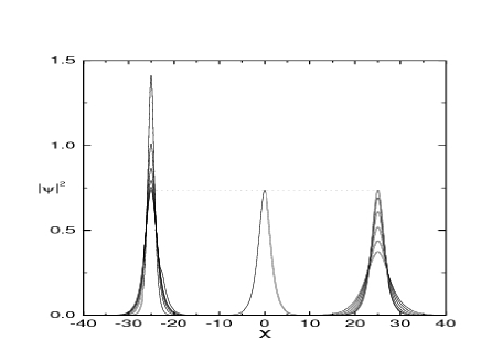
Figure 1: Early stages of the evolution toward collapse (left curves) or decay (right curves) of the critical soliton (central curve) in absence of external potentials ($\alpha=0,\varepsilon=0$). The critical soliton in the center refers to the value $\chi=-1$ and $N=2.7207$, while the collapse and the decay evolution refer to $\chi=-1.01$ and $\chi=-0.99$, respectively, with all other parameters unchanged. Snapshots were taken at regular time intervals of $5.2$ for collapse and of $10$ for decay. Plotted quantities are in normalized units.

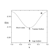
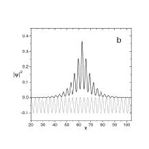
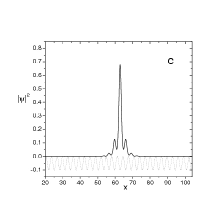
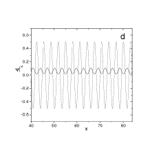
Figure 2: Panel a. Lower band and localized bound states of the quintic NLS with attractive interactions for parameter values $\chi=-1$, $\varepsilon=5$. The arrows show the decay pattern of the Townes bound state (open circle) for $N<N_{cr}$ (upper arrow) and $N>N_{cr}$ (lower arrow). Panel b. Townes soliton (thick line) corresponding to the unstable bound state level (open circle) in panel a, with $N=N_{cr}=0.4616$ and $E=-2.1576$. Panel c. Gap soliton (thick line and filled circle in panel a) obtained from the unstable Townes state for a slightly above critical value of $N$ ($N=0.4657,E=-2.2177$). Panel d. The Bloch state (thick line) at the bottom of the band into which the Townes soliton decays for a slightly sub-critical value of $N$ ($N=0.4586,E=-2.1531$). The OL is depicted as a thin dotted line scaled by a factor 100 and shifted down by $.05$ in panel b,c, and scaled by a factor $10$ in panel d. Plotted quantities are in normalized units.

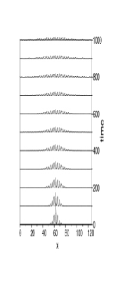
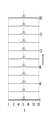
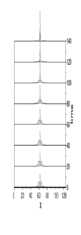
Figure 3: Time evolution of the Townes soliton in Fig.2 (central panel) compared with the one obtained from numerical integration of the quintic NLS with two slightly different values of $N$: $N=1.1N_{cr}$ (right panel) and $N=0.9N_{cr}$ (left panel). Parameters are fixed as in Fig. 2 and plotted quantities are in normalized units.

III Attractive interactions

To obtain analytical predictions for the existence of stable localized solutions of Eq.(5) with $\alpha=0$ and for attractive interactions ($g,\chi<0$ in Eq.(5)), we use the variational approximation (VA) with a Gaussian ansatz for the fundamental soliton

$$\psi(x,t)=A\exp\left(-i\mu t-\frac{1}{2}ax^{2}\right),$$ (9)

with $\mu$ denoting the chemical potential and $A$, $a$, the amplitude and the square root of the reciprocal width of the soliton, respectively. Following the standard VA (see Mal for a review) we derive the following effective Lagrangian

$$\bar{L}=\frac{A^{2}\sqrt{\pi}}{2\sqrt{a}}\left(\mu-\frac{a}{2}+\varepsilon e^{-1/a}-\frac{gA^{2}}{2\sqrt{2}}-\frac{\chi A^{4}}{3\sqrt{3}}\right),$$ (10)

from which the stationary equations $\partial\bar{L}/\partial a=\partial\bar{L}/\partial A=0$ for parameters $a$ and $A$ are obtained as

$$\mu=-\frac{a}{2}(1-\frac{2N^{2}\chi}{3^{3/2}\pi})+\varepsilon(\frac{2}{a}-1)e^{-1/a}+\frac{gN\sqrt{a}}{2\sqrt{2\pi}},$$ (11)

$$\frac{2N^{2}\chi}{3^{3/2}\pi}+\frac{gN}{2\sqrt{2\pi a}}=\frac{2\varepsilon}{a^{2}}e^{-1/a}-1.$$ (12)

Here the number of atoms has been expressed in terms of $a,A,$ as $N=A^{2}\sqrt{\frac{\pi}{a}}$. Note that for $\varepsilon=0,g=0$, Eqs. (12) predicts a maximum value of $N$ for the existence of soliton given by $N_{cr}=\sqrt{3^{3/2}\pi/(2\chi)}$. This value should be compared with the critical norm $N_{cr}^{(e)}=(\pi/2)\sqrt{3/|\chi|}$ obtained for the exact Townes soliton of Eq. (5) with $\varepsilon=0,g=0,\alpha=0$, Gaididei

$$\psi_{s}=\exp(i\mu t)\psi,\;\;\;\psi=\frac{(3\mu/|\chi|)^{1/4}}{\sqrt{\mbox{cosh}(2\sqrt{\mu}x)}}.$$ (13)

We see that the VA value deviates from the exact one by only $5\%$. Notice that the above solution has zero energy and is marginally stable ($dN/d\mu=0$) so it exists only for the single value of the norm $N=N_{cr}^{(e)}$. Since for $N>N_{cr}^{(e)}$ the solution collapses in a finite time, while for $N<N_{cr}^{(e)}$ it decays into the uniform background, it appears as the analogue of the Townes soliton of the cubic 2D NLS equation with attractive interactions. In Fig.1 we depict the early stages of the time evolution toward collapse (decay) for an initial norm which is slightly increased (decreased) with respect to $N_{cr}^{(e)}$.

For $\varepsilon\neq 0$ Eq. (12) shows that the number of particles attains a minimum value $N_{{\rm thr}}=\left[6\pi\sqrt{3}(1-8\varepsilon e^{-2})\right]^{1/2}$ at $a=1/2$, i.e. there exists a threshold value of the norm which is necessary to create a soliton. The expression for $N_{{\rm thr}}$ shows that the threshold exists for a relatively weak lattice and disappears if $\varepsilon$ exceeds the value $\varepsilon_{0}=e^{2}/8\approx\allowbreak 0.\,\allowbreak 9236$. From this analysis it is clear that the optical lattice is quite effective to stabilize solitons against decay when $N$ is in the interval $N_{{\rm thr}}<N<N_{{\rm cr}}$. Collapse and decaying into extended states is expected for $N>N_{{\rm cr}}$ and $N<N_{{\rm thr}}$, respectively. The VA makes it possible to predict stability of the solitons on the basis of the Vakhitov-Kolokolov (VK) criterion Berge , according to which a necessary condition for stability is given by $d\mu/dN<0$. Notice that the above variational equations are very similar to the ones derived in Ref. bms03 for the 2D cubic NLS (with exactly the same value of $\varepsilon_{0}$), this being a further confirmation of the analogy between the 1D quintic NLS and the usual 2D GPE. We remark that, since $N_{cr}$ does not dependent on $\varepsilon$, the prediction of the VA is that the optical lattice does not affect collapse. We shall check these results in the next section.

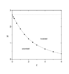
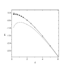
Figure 4: Left Panel. Delocalizing transition threshold obtained by direct numerical integrations (filled dots) of the quintic NLS with $\chi=-1.0$. The horizontal dotted line corresponds to the critical threshold for collapse in absence of the OL: $N_{cr}=\frac{\pi}{2}\sqrt{\frac{3}{\chi}}$. Right Panel. Energies versus $\varepsilon$ of the gap soliton (bottom curve with open squares), Townes soliton (middle curve with filled circles) and Bloch state at the bottom of the band (top curve with open circles) for the quintic NLS with $\chi=-1.0$. Plotted quantities are in normalized unit.

IV Gap-Townes solitons and arresting collapse in 1D BEC in OL

The existence of the exact Townes soliton (13) of the quintic NLS with $\varepsilon=0$ makes natural to ask whether this solution could exist also in presence of the OL. In view of the analogies between 1D quintic NLS and 2D GPE, the existence of this solution for $\varepsilon\neq 0$ could shine some light on the role of the OL in controlling collapse, as well as, on the origin of the delocalizing transition observed in these systems BS . In the following we use a self consistent approach salerno to determine the critical value of $N$ for the unstable solution to exist.

In Fig.2a we report the band structure and the localized states obtained with the self-consistent approach for the case $g=0,\alpha=0$ in Eq. (5). We see that there are two bound state levels just below the band. The level closer to the band edge (open circle) corresponds to an unstable localized state while the other corresponds to a stable gap soliton. The corresponding wavefunctions are depicted in Figs. 2b,c, respectively. We find that for a fixed value of $\varepsilon$ there is only one value $N$ for which the unstable state exists and its behavior resembles the one of the Townes soliton depicted in Fig. 1. In this case, however, we have that for a slightly overcritical value of N the unstable soliton starts to shrink and its energy decreases as for collapsing solutions until it reaches the gap soliton level below, at which the shrinking stops. The transition from the unstable Townes soliton to the stable gap soliton is represented in Fig.2a by the lower arrow. If the norm is slightly decreased below $N_{cr}$ the unstable state completely delocalizes into the Bloch state at the bottom of the band shown in Fig.2d (this decay is represented in Fig.2a by the upper arrow). Due to this behavior we refer to the unstable state as gap-Townes soliton, this name being also justified by the fact that for $\varepsilon\rightarrow 0$ the critical norm reduces to $N_{cr}^{e}$ (see left panel of Fig. 4). The decaying property of the gap-Townes soliton is illustrated in Fig.3 where the time evolution obtained from direct numerical integrations of Eq. 5 (with $g=0,\alpha=0$) is shown. The left (right) panel of this figure shows the decay into the extended state (gap soliton) when the initial norm is slightly decreased (increased) with respect to $N_{cr}$. Notice that the transition into the gap soliton state is much more rapid than the decay into the extended state, this being a reminiscence of the collapse occurring at $\varepsilon=0$. Since the energy of a slightly overcritical gap-Townes solution should go to $-\infty$, as for any collapsing solution, we see that the existence of a stable localized state which lies in energy below the unstable state is indeed a mechanism for arresting collapse in the system.

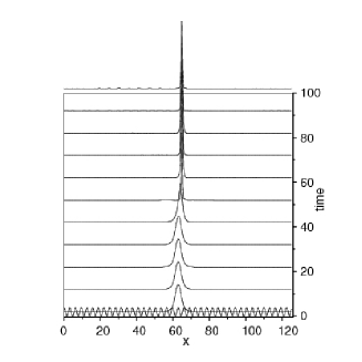
Figure 5: Time evolution of an intersite symmetric intrinsic localized mode for the attractive case $\chi=-1$ with $N=2.847$ and $\epsilon=0.1$. Notice that collapse starts after the mode has decayed into an onsite symmetric one (ground state). The periodic potential is shown together with the initial state at $t=0$. Plotted quantities are in normalized unit.

Also note that a gap-Townes soliton appears as a separatrix between localized and extended states. The fact that its energy lies below the lower band edge implies the existence of a delocalizing threshold in the number of atoms below which localized state of the quintic GPE with OL cannot exist, this being a remarkable difference between cubic and quintic nonlinearities (in the cubic case the threshold exists only in the higher dimensional case BS ). In Fig. 4a the threshold curve separating localized and extended states in the $(N,\varepsilon)$ plane is depicted (this curve coincides with the norm of the gap-Townes soliton as a function of $\varepsilon$). Notice that for $\varepsilon=0$ the norm coincides with the exact value $N_{cr}^{(e)}$ of the solution in (13), suggesting that the family of gap-Townes soliton for $\varepsilon\neq 0$ originates from the Townes soliton state at $\varepsilon=0$.

Numerical investigations show that collapse occurs when the strength of the optical lattice becomes small and the number of atoms overcomes the critical threshold for Townes soliton at $\varepsilon=0$. For larger values of $N$ the width of the soliton becomes small compared to the period of the periodic potential and the OL becomes ineffective for arresting collapse. We find that solitons extended on several potential wells are the ones which are better stabilized by the optical lattice against collapse. An indication of occurrence of collapse at small values of $\varepsilon$ is obtained from the right panel of Fig. 4 in which we depict the energies of the Bloch state at the bottom of the band, of the gap-Townes soliton immediately below the band and of the gap soliton, are reported as a function of $\varepsilon$. We see that while the energies of the Bloch state and of the gap- Townes soliton monotonically increase with decreasing $\varepsilon$, the energy of the gap soliton reaches a maximum around $\varepsilon\approx 1$ and then starts to decrease as $\varepsilon\rightarrow 0$. This behavior is consistent with the fact that a collapsing solutions with energy equal to $-\infty$ should exist at $\varepsilon=0$. A study of collapse for small $\varepsilon$ is numerically difficult to perform and requires more investigations. It is interesting to note, however, that besides stable gap-soliton the OL allows the existence of metastable states which are symmetric around a maximum of the potential (instead than a minimum as for usual gap-solitons). These intersite symmetric states have higher energy than the onsite symmetric ones and decay into the ground state after some time. Such states can be used to delay the time of collapse for $N>N_{{\rm cr}}$. Indeed, the collapse of these metastable states begins when their instability sets in, as one can see from Fig. 5 (notice that the matter moves first into a single potential well and then starts to collapse).

V Repulsive interactions

To investigate the existence of localized states in the repulsive quintic NLS with periodic potential we apply first a variational analysis based on the following ansatz for the soliton waveform BS

$$\psi(x,t)=A\frac{\sin(ax)}{ax}\exp\left(-i\mu t\right).$$ (14)

Performing the same analysis as before, we get the averaged Lagrangian

$$\bar{L}=\frac{A^{2}\pi}{2a}\left(\mu-\frac{a^{2}}{3}+\varepsilon(1-\frac{1}{a})-\frac{11\chi A^{4}}{60}-\frac{gA^{2}}{3}\right)$$ (15)

from which the following equations for the soliton parameters are obtained

$$\mu=\varepsilon(\frac{2}{a}-1)-\frac{1}{3}a^{2}+\frac{11\chi N^{2}a^{2}}{60\pi^{2}}+\frac{gNa}{3\pi},$$ (16)

$$\frac{N^{2}\chi}{\pi^{2}}+\frac{10gN}{11\pi a}=\frac{20}{11}(\frac{3}{2}\frac{\varepsilon}{a^{3}}-1).$$ (17)

Using the fact that the norm and the soliton parameters are related by $N=\pi A^{2}/a$, one can show that

$$A=\Bigl{[}\frac{30N^{3}\varepsilon}{2\pi(11N^{2}|\chi|+20\pi^{2})}\Bigr{]}^{1/6},$$ (18)

i.e. the VA predicts the existence of a single set of soliton parameters $a,A$ for a given norm $N$ and strength $\varepsilon$ of the OL. This is similar to what obtained in Ref. BS for the localized solutions of the repulsive 2D GPE with OL.

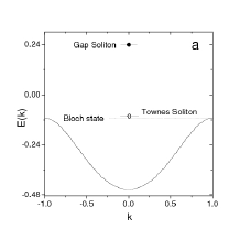
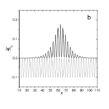
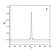
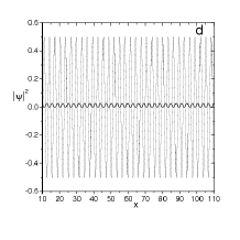
Figure 6: Panel a. Lower band and localized bound states of the quintic NLS with repulsive interactions for parameter values $\chi=1$, $\varepsilon=2.0$. The arrows show the decay pattern of the Townes bound state (open circle) for $N<N_{cr}$ (upper arrow) and $N>N_{cr}$ (lower arrow). Panel b. Townes soliton (thick line) corresponding to the unstable bound state level (open circle) in panel a, with $N=N_{cr}=1.5565$ and $E=-0.1047$. Panel c. Gap soliton (thick line and filled circle in panel a) obtained from the unstable Townes state for a slightly above critical value of $N$ ($N=1.5965,E=0.2537$). Panel d. The Bloch state (thick line) at the bottom of the band into which the Townes soliton decays for a slightly sub-critical value of $N$ ($N=1.5065,E=-0.1097$). The OL is depicted as a thin dotted line scaled by a factor 20 and shifted down by $.05$ in panel b,c, and scaled by a factor $10$ in panel d. Plotted quantities are in normalized units.

In the case of a Tonks-Girardeau gas in OL these parameters can be estimated as follows . From Eq.(18) we get that $A\approx(30N\varepsilon/22\pi)^{1/6}$ and from the expression of $N$ we get for the soliton width $w=1/a\approx(22N^{2}/(30\pi^{2}\varepsilon))^{1/3}.$ For a number of particles $N=314$ (corresponding in physical units to $N_{p}=100$) and for $V_{0}=4E_{R}$,so $\varepsilon=2$, the width of the gap soliton is estimated to be $w\approx 15.5$ corresponding to $3-4$ lattice periods.

The band structure associated to gap solitons of the repulsive quintic NLS equation has been investigated by means of the self-consistent method. In Fig. 6a we show the lower band and the localized bound states for the case $g=0,\alpha=0$ in Eq. (5). We see that above the band edge there are two bound state levels, one immediately above (open circle) corresponding to an unstable gap-Townes soliton, the other more separated from the band edge corresponding to a gap soliton. The wavefunctions of these bound states are depicted in Figs. 6b,c. In analogy with the attractive case, we have that the unstable soliton exists only for a critical value $N_{cr}$ of the norm and has a behavior similar to the gap-Townes soliton described before. The decaying property of the repulsive gap-Townes soliton is clearly illustrated in Fig.7 where we show the time evolution, as obtained from direct numerical integrations of Eq.5 (with $g=0,\alpha=0$), of the gap-Townes soliton in Fig.6b (central panel). The left and right panels of this figure show the decays into the extended (Bloch) and localized state (gap soliton) when the norm of the initial condition is, respectively, slightly decreased or increased with respect to $N_{cr}$.

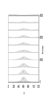
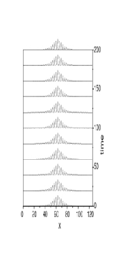
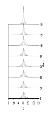
Figure 7: Time evolution of the Townes soliton in Fig.6 as obtained from numerical integration of the quintic NLS with repulsive interaction and three slightly different values of number of atoms: $N_{cr}=1.5565$ (central panel), $N=1.05N_{cr}$ (right panel) and $N=0.95N_{cr}$ (left panel). Other parameters are fixed as in Fig.6. Plotted quantities are in normalized units.

Thus, also in this case a gap-Townes soliton appears as a separatrix between localized and extended states. We remark, however, that in this case the existence of gap-solitons is a direct consequence of the band structure (it could not exist without the OL). The fact that the energy of the Townes soliton is slightly above the upper band edge is consistent with the existence of a threshold in the number of atoms (given by the critical norm of the gap-Townes soliton) below which localized state of the quintic GPE with OL cannot exist. In the left panel of Fig. 8 we show the delocalizing curve in the plane $(N,\varepsilon)$ separating localized from extended states. This behavior is very similar to what reported for repulsive 2D solitons of the GPE in optical lattices BS . In the right panel of the same figure we show the energies of the Bloch states at the top of the band, of the Townes soliton immediately above the band and of the gap soliton, as a function of $\varepsilon$. In contrast with the attractive case we see that all energies monotonically increase with decreasing $\varepsilon$. The absence of a maximum in the energy curve of the gap soliton at small values of $\varepsilon$ also indicates the absence of collapse in this case (compare the right panels of Figs 4 and 8).

VI Gap-Townes solitons in presence of dissipation

In the previous sections we have investigated the general properties of localized states of 1D BEC in OL with the elastic three-body interactions modeled by a real quintic nonlinearity. It is known, however, that the three-body interactions bears also an imaginary component corresponding to inelastic collisions which can be modeled by a damping term of the form $-i\gamma|\psi|^{4}\psi$ in the right hand side of Eq. (5). Recent theoretical studies Bed -Koh estimate for $Rb$ a negative value of the real part of the quintic nonlinearity of the order of $10^{-26}-10^{-27}cm^{6}/s$ . From the experiment in Ref. Tolra one can deduce the imaginary part of the three-body interaction for $Rb$ to be of the order $10^{-30}cm^{6}/s$. These numbers imply a ratio between the imaginary and the real part of this interaction of the order $10^{-3}-10^{-4}$. Other data gives values of the damping constant of the order $10^{-28}cm^{6}/s$. Due to the uncertainty intrinsic in some of these numbers (presently there are no measurements of the real part of the three-body interactions) in the following we take the damping constant $\gamma$ to be a free parameter and investigate both the underdamped and the overdamped regimes.

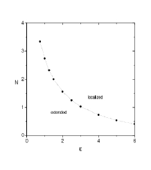
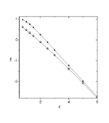
Figure 8: Left Panel. Delocalizing transition threshold obtained by direct numerical integrations (filled dots) of the quintic NLS with $\chi=1.0$. Right Panel. Energies versus $\varepsilon$ of the gap soliton (top curve with filled triangles), Townes soliton (curve with filled circles) and Bloch state at the top of the band (curve with open circles) for the quintic NLS with $\chi=1.0$. Plotted quantities are in normalized units.

The instability of gap-Townes solitons against small fluctuations in the number of the atoms rises the question of how the scenario of the previous sections changes in presence of dissipation. To answer this question we concentrate on the case of attractive quintic interactions (qualitatively similar results holds also for repulsive interactions) in presence of a quintic dissipation. The results are displayed in Fig. 9. In the top three panels of this figure we depict the time evolution of the Townes soliton in Fig. 2 in presence of a small damping. We see that in spite of a slow broadening of the Townes soliton (middle panel), the situation remains qualitatively similar to the undamped case depicted in Fig. 3. Notice that for an overcritical number of atoms (right top panel) several focusing-defocusing cycles between the gap-Townes soliton and the gap soliton occur (these oscillations are induced by the slightly overcritical starting value of $N$). From the left panel of this figure we also see that for an undercritical number of atoms the decay into the Bloch states occurs faster than for the zero damping case. At very long times the gap-Townes soliton in the middle panel of Fig. 9 eventually decays into the Bloch stated at the edge of the band.

For larger damping the situation is different, as one can see from the bottom three panels of Fig.9. Notice that for an overcritical value of $N$ the gap-Townes soliton (right panel) decays into an extended state after performing only one focusing-defocusing cycle. In this case the dissipation completely suppresses collapse and localized states becomes unstable against decay into the lowest energy Bloch state. It is remarkable, however, that a signature of the existence of gap-Townes soliton remains even for moderately large dampings in the focusing defocusing cycles observed when the decreasing (due to dissipation) number of atoms crosses the critical value for existence of gap-Townes soliton. This fact could indeed be used in experiments to detect the existence of gap-Townes solitons in presence of damping.

An analytical explanation of the existence of focusing-defocusing cycles can be obtained by means of a modified variational analysis Bendenson ; FAGT in which the damping is treated as a small perturbation. In this approach we assume a time dependent localized state of the form

$$\psi(x,t)=A\exp(-\frac{x^{2}}{2w^{2}}+ibx^{2}+i\phi),$$ (19)

with parameters $\eta_{i}\equiv\{A,w,b,\phi\}$ also time dependent. The equations of motion for these variables are obtained from the averaged unperturbed Lagrangian of Eq.(5) with $g=0$

$$L=-\frac{\sqrt{\pi}}{2}A^{2}w[w^{2}b_{t}+2\phi_{t}+\frac{1}{w^{2}}+4w^{2}b^{2}-2\varepsilon e^{-w^{2}}+\frac{2\chi}{3\sqrt{3}}A^{4}]$$

as

$$\frac{d}{dt}\frac{\partial L}{\partial{\eta_{i,t}}}-\frac{\partial L}{\partial\eta_{i}}=\int_{-\infty}^{\infty}dx(R\psi^{\ast}_{\eta_{i}}+R^{\ast}\psi_{\eta_{i}})$$ (20)

where $R=-i\gamma|\psi|^{4}\psi$, and the subscript ${\eta_{i}}$ denotes the derivative with respect to soliton parameters. From the above generalized Euler-Lagrange equation one derives the following equations for the number of atoms $N$ and soliton width $w$

$$N_{t} = -3\gamma\beta\frac{N^{3}}{w^{2}},$$

$$w_{tt} = \frac{4}{w^{3}}(1+\chi\beta N^{2})-8\epsilon we^{-w^{2}},$$ (21)

with $\beta=2/(3\sqrt{3}\pi).$

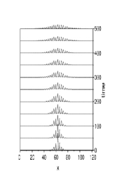
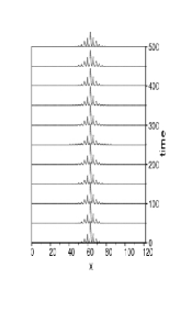
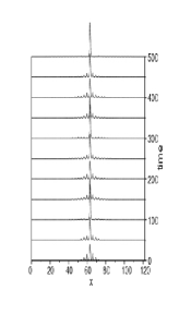
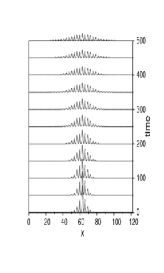
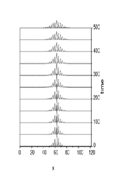
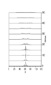
Figure 9: Time evolution of Townes soliton in Fig.2 as obtained from numerical integration of the dissipative quintic NLS with attractive interaction. The top three panels refer to three slightly different values of number of atoms: $N_{cr}=0.87248$ (central panel), $N=1.1N_{cr}$ (right panel) and $N=0.9N_{cr}$ (left panel) with a dissipation parameter $\gamma=0.00025$. The bottom three panels are the same but for $\gamma=0.01$. Other parameters are fixed as $\chi=-1$, $\varepsilon=5$. Plotted quantities are in normalized units.

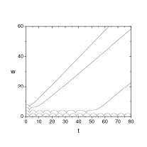
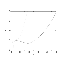
Figure 10: Left panel. Time evolution of the width of the Townes soliton as obtained from Eqs. VI with $\varepsilon=2$, $\chi=-1$ and damping parameters increased by a factor $10$ going from the bottom curve ($\gamma=0.0001$) to the top one ($\gamma=0.1$). The last three curves have been shifted respectively by $2,4,6$, to avoid overlapping. The initial value of atoms was detuned from the critical value $N=1.254$ corresponding to the unperturbed Townes by $0.05$. Right panel. Time evolution of the soliton width obtained from the damped quintic GPE (continuous line) and from the variational equations VI (dotted line). Parameter values are taken as $\varepsilon=2$, $\chi=-1$, $\gamma=0.01$. The comparison with the variational results was done by rescaling the soliton width obtained from the GPE by a factor $11.5$ to have the same initial condition. Plotted quantities are in normalized units.

In Fig 10 we show the time evolution of the soliton width for different values of the dissipation constant. We wee that for very low dampings the width oscillates around a constant value, meaning that the localized state undergoes periodic focusing-defocusing cycles in agreement with the right top panel of Fig. 9. By increasing the damping we see that after a certain number of cycles, the soliton width starts to grow monotonically signaling the decay of the gap soliton into an extended state. Notice that even for relatively high dampings there is one focusing-defocusing cycle, this being in good qualitative agreement with what observed in the bottom right panel of Fig. 9. In the right panel of Fig. 10 we make a quantitative comparison between the dynamics of the soliton width as obtained from the VA and from the damped quintic NLS. From this figure we see that although the main feature of the phenomenon is correctly captured (i.e. existence of only one focusing-defocusing cycle before decay), the variational equations are not in good quantitative agreement with the numerical integration of the full system. This may be due to the fact that the ansatz in Eq.(19) is more appropriate for strongly localized states than for extended gap-Townes ones. It is interesting, however, that for $\epsilon=0$ the variational equations become similar in form to the ones considered for the 2D cubic NLSE in presence of a cubic dissipation $-i\gamma|\psi|^{2}\psi$ Fibich . In this case one can show that the equation for $w$ reduces to a modified Airy equation for which a focusing-defocusing cycle always exists. When $\epsilon\neq 0$, Eq.s (VI) predict that for decreasing $\gamma$ the number of focusing-defocusing cycles grows, this being in good agreement with direct numerical simulations. Moreover, from the left panels of Figs. 4 and 8 we see that the critical value of the number of atoms for existence of gap-Townes soliton decreases by increasing $\varepsilon$, this meaning that in strong optical lattices the effect of the quintic damping on gap-Townes solitons is effectively reduced (due to the reduced norm), this being confirmed also by numerical simulations.

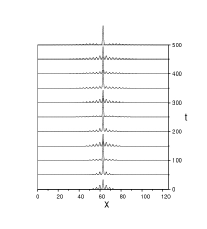
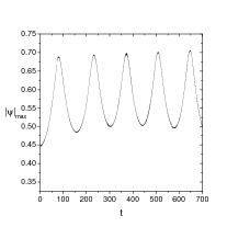
Figure 11: Left panel. Time evolution of the gap-Townes soliton in the lower right panel of Fig. 9 in presence of quintic dissipation $\gamma=0.01$ and linear amplification of strength $\delta=8.95\cdot 10^{-4}$. Right panel. Time evolution of the gap-Townes soliton amplitude in the left panel. Plotted quantities are in normalized units.

We remark that besides the decay phenomena induced by the quintic dissipation one could also consider the feeding of atoms in the condensate from the thermal cloud kagan . The injection of matter in the condensate can be modeled with a linear imaginary term (of sign opposite to $\gamma$) in the NLS equation of the form $i\delta\psi$. This term can balance the damping and stabilize localized states against decay even in the overdamped regime, this leading to the formation of dissipative gap solitons. We illustrate this phenomenon in Fig. 11 where the time evolution of the slightly overcritical gap-Town soliton shown in the bottom right panel of Fig. 9 is reported for a linear amplification term of strength $\delta=8.95\cdot 10^{-4}$. From this figure we see that the localized state instead of decaying into the Bloch state at the bottom of the band (see Fig. 9), it executes breather-like oscillations (i.e. focusing-defocusing cycles) with emission of radiation. In terms of band picture this breathing state can be thought as a non stationary states with energy oscillating between the gap-Townes soliton and the gap soliton in Fig. 2a. We believe this being a general mechanism for existence of breather-like excitations in 1D BEC in OL in presence of damping and amplification.

VII Conclusions

In this paper we have used the periodic 1D NLS equation with quintic nonlinearity to investigate localized states in 1D BEC in OL with three-body interactions. The existence of unstable solitons similar to the usual Townes soliton of the cubic 2D NLS has been established. These states have been shown to have energy located in the forbidden zones of the band structure, very close to band edges, separating decaying states from stable localized ones (gap-solitons). The existence of gap solitons appears to be a mechanism for arresting collapse in attractive low dimensional BEC with three-body interactions in OL and the analysis of gap-Townes solitons appears to be important for characterizing the delocalizing transition in these systems. To this regard we remark that the region of existence of localized states in the $N,\varepsilon$ plane is bounded by two limiting curves. The first curve separates extended states from localized ones and therefore characterizes the delocalizing transition. This curve coincides with the curve of existence of gap-Towenes solitons. For the 1D quintic NLS with periodic potential the delocalizing transition exists for both attractive and repulsive interactions. Delocalizing curves have been investigated in Fig.s 4, 8. A similar behavior is expected to be valid also for the standard GPE with periodic potential in higher dimensions. The second curve separates the localized solutions from the collapsing ones, giving an upper bound for the existence of gap-solitons. This curve obviously exists only for attractive interactions (for repulsive interactions a negative effective mass, although producing an attraction among atoms which leads to the formation of gap solitons, is usually insufficient to induce collapse). Due to the numerical difficulties involved in the study of collapsing solution, the threshold curves for collapse have not been investigated in this paper. For this it will be useful to develop an analytical approach to provide estimates of the critical values for collapse Kon2 .

We have also investigated the influence of a dissipative imaginary part of the three-body interaction on gap-Townes solitons. In particular, we have shown that the damping introduces effects which are important when the ratio between the imaginary and the real part of the three-body interaction is not small. For the case of rubidium this ratio is expected to be small and the situation described for the underdamped case should be qualitatively valid. It is remarkable, however, that even for moderate large damping a signature of the existence of gap-Townes solitons remains in the focusing-defocusing cycles observed when the number of atoms crosses the critical value for their existence.

Finally, we have shown that the presence of a small linear amplification term into the damped quintic NLS equation, modelling the feeding of atoms from the thermal cloud, can stabilize gap solitons into breather-like excitations even in presence of large damping.

The results of this paper suggest the possibility to experimentally observe gap-Townes solitons in low dimensional BEC.

- (1) B.P. Anderson and M.A. Kasevich, Science, 282, 1686 (1998).
- (2) M. Cristiani, J. Morsch, J. Miller, D. Ciampini, and E. Arimondo, Phys.Rev. A 65, 63612 (2002).
- (3) B. Wu and Q. Niu, New J. Phys., 5, 104 (2003).
- (4) B. Eiermann, et al., Phys.Rev.Lett., 91, 060402 (2004).
- (5) M. Greiner, O. Mandel, T. Esslinger, T.W. Hansch, and I. Bloch, Nature, 415, 39 (2002).
- (6) B.B. Baizakov, V.V. Konotop, and M. Salerno, J.Phys. B:At.Mol.Opt.Phys., 35 , 5105 (2002).
- (7) E. Ostrovskaya and Yu.S. Kivshar, Phys.Rev.Lett., 90, 160407 (2003).
- (8) N. Akhmediev et al., Int.J.Mod.Phys.B 13, 625 (1999).
- (9) W. Zhang, E.M. Wright, H. Pu, and P. Meystre, Phys.Rev. A 68, 023605 (2003).
- (10) F.Kh. Abdullaev, A. Gammal, L. Tomio, and T. Frederico, Phys.Rev. A 63, 043604 (2001).
- (11) A. Gammal, T. Frederico, L. Tomio, and F.Kh. Abdullaev, Phys.Lett. A 267, 305 (2000).
- (12) S. Inouye, M. R. Andrews, J. Stenger, H. J. Miesner, D. M. Stampur-Kurn and W. Ketterle, Nature (London) 392, 151 (1998).
- (13) V. Efimov, Phys.Lett. 33B, 563 (1970).
- (14) A. Bulgac, Phys.Rev.Lett. 89, 050402-1-4 (2002).
- (15) P.F. Bedaque, E. Braaten, and H -W. Hammer, Phys.Rev.Lett. 85, 908 (2000).
- (16) P.F. Braaten and H -W. Hammer, Phys.Rev.Lett. 88, 040401 (2001).
- (17) Jack W. Michael, Phys.Rev.Lett. 89, 140402 (2002).
- (18) T. Köhler, Phys.Rev.Lett. 89, 210404 (2002).
- (19) E.B. Kolomeisky, T.J. Newmann, J.P. Straley, and Qi Xiaoya, Phys.Rev.Lett. 85, 1146 (2000).
- (20) A. Minguzzi, P. Vignolo, M.I. Chiofalo, and M.P. Tosi, Phys.Rev. A 64, 033605 (2001).
- (21) B. Damski, J.Phys. B:At. Mol. Opt. Phys. 37, L85 (2004).
- (22) D.J. Frantzeskakis, N.P. Proukakis, and P.G. Kevrekidis, Phys.Rev.A 70 , 015601 (2004).
- (23) M.D. Girardeau and E.M. Wright, Phys.Rev.Lett. 84, 5239 (2000).
- (24) L. Berge, Phys.Rep. 303, 259 (1998).
- (25) V.A. Brazhnyi and V.V. Konotop, Modern.Phys.Lett. B 18, 627 (2004).
- (26) B.V. Gisin, R. Driben, and B.A, Malomed, J.Opt.B:Quantum Semiclass.Opt. 6, S259 (2004).
- (27) C. De Angelis, IEEE J.Quant.Electron., 30, 818 (1994).
- (28) K.D. Moll, A.L. Gaeta, and G. Fibich, Phys.Rev.Lett. 90, 203902 (2003).
- (29) B.A. Malomed, Progress in Optics, 43, 69 (2001).
- (30) Mario Salerno, Laser Physics 15, No.4, 620 (2005); see also cond-mat/0311630.
- (31) Yu.B. Gaididei, J. Schjodt-Eriksen, and P.L. Christiansen, Phys.Rev. E 60, 4877 (1999).
- (32) B.B. Baizakov, B.A. Malomed, and M. Salerno, Eurphys.Lett. 63, 642 (2003).
- (33) B.B. Baizakov and M. Salerno, Phys.Rev. A 69, 013602 (2004).
- (34) B.L. Tolra, K.M. O’Hara, J.H. Huckans, W.D. Phillips, S.L. Robston, and J.V. Porto, Phys.Rev.Lett. 92, 190401 (2004).
- (35) A. Bondeson, M.Lisak, and D. Anderson, Phys.Scr. 20, 479 (1979); A. Maimistov, Zh.Eksp.Teor.Fiz 104, 3620 (1993) [JETP 77, 727 (1993)].
- (36) V. Filho, F.Kh. Abdullaev, A. Gammal, and L. Tomio, Phys.Rev. A 63, 053603 (2001).
- (37) G. Fibich, SIAM J.Appl.Math. 61, 1680 (2001).
- (38) Y.Kagan, A.E. Muryshev, and G.V. Shlyapnikov, Phys.Rev.Lett. 81, 933 (1998).
- (39) V.V. Konotop and P. Pacciani, private communication.