Nonergodisity of a time series obeying Lévy statistics

Abstract

Time-averaged autocorrelation functions of a dichotomous random process switching between 1 and 0 and governed by wide power law sojourn time distribution are studied. Such a process, called a Lévy walk, describes dynamical behaviors of many physical systems, fluorescence intermittency of semiconductor nanocrystals under continuous laser illumination being one example. When the mean sojourn time diverges the process is non-ergodic. In that case, the time average autocorrelation function is not equal to the ensemble averaged autocorrelation function, instead it remains random even in the limit of long measurement time. Several approximations for the distribution of this random autocorrelation function are obtained for different parameter ranges, and favorably compared to Monte Carlo simulations. Nonergodicity of the power spectrum of the process is briefly discussed, and a nonstationary Wiener-Khintchine theorem, relating the correlation functions and the power spectrum is presented. The considered situation is in full contrast to the usual assumptions of ergodicity and stationarity.

I Introduction

Many time series exhibit a random behavior which can be represented by a two-state process Allegrini-wrong . In such processes the state of the system will jump between state on and state off. Examples include ion channel gating dynamics in biological transport processes NadlerStein91 ; GoychukHanggi02 and gene expression levels Dewey02 ; Roy in cells, neuronal spike trains Masuda , motion of bacteria Korobkova04 , fluorescence intermittency of single molecules Haase04 and nanocrystals Nirmal ; Kuno ; Ken ; Brokmann ; Dahan , and fluorescence fluctuations of nanoparticles diffusing through a laser focus Zumofen04 . Some aspects of spin dynamics can also be characterized using two distinctive states GL ; Bald . These diverse systems may display non-ergodicity and/or Lévy statistics BouchaudGeorges90 ; Schlesinger ; MetzKlaf00 ; BJS04 , and often their behavior is found to deviate from simple scenarios used in the past to interpret the behavior of ensembles. In particular, in certain systems Nirmal ; Kuno ; Ken ; Brokmann ; Dahan ; NadlerStein91 ; Korobkova04 ; Haase04 ; GL ; Bald ; Zumofen04 power law sojourn times are found for one or both of the states. Lévy statistics, which manifests itself in appearance of power laws, is also found in flows on chaotic maps ZK , which may be used to model dynamics of various complex systems with non-linear interactions. In this paper we address non-ergodicity of the Lévy walk processes using a stochastic approach.

We model the intermittent behavior by a random process which switches between the two states after random sojourn times drawn from the probability density functions (PDFs) $\psi_{\pm}(\tau)$, where the $\pm$ denote the two states (see Fig. 1).

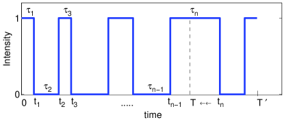
Figure 1: Schematic representation of a dichotomous process. $T=T^{\prime}-t^{\prime}$, where $T^{\prime}$ is the duration of the experiment and $t^{\prime}$ is the time difference used in correlation function (see Eq. (2)). Note that in Section V we redefine $t_{n}$ to be equal to T and $\tau_{n}$ is redefined to be $T-t_{n-1}$, to simplify notation.

It is assumed that these sojourn times are mutually independent random variables. In the following we assume common PDF for both states $\psi(\tau)$, unless stated otherwise, and assume that in state $+$, or on, the system is described by the intensity $I=1$, while in state $-$, or off, it is described by zero intensity, $I=0$ (Fig. 1). We consider the case of power law decay for long times

$$\psi(\tau)\sim\theta\tau^{-1-\theta},\,\,\,\,\,0<\theta<1,$$ (1)

where we use natural units with dimensionless $\tau$. Such distributions are observed in nanocrystal experiments Nirmal ; Kuno ; Ken ; Brokmann ; Dahan , which under continuous laser illumination exhibit random two-state blinking. As the mean sojourn time diverges, this situation reflects aging and non-ergodicity. Aging means dependence of some observables (e.g., ensemble average correlation functions) on absolute times from the process onset at time zero, even in the limit of long times Marinari93 ; Chaos ; Cheng ; MB_JCP ; Bouchaud92 ; LineShape04 . Non-ergodicity means that ensemble averages are not equal to time averages of single realizations, even in the limit of long times.

Generally speaking, our model represents the so-called Lévy walk process MetzKlaf00 , in which a particle travels on a line with a constant velocity, changing directions at random times; the sojourn times are distributed with a power-law decaying PDF $\psi(\tau)$. Some of the systems mentioned above can in certain aspects be viewed as physical realizations of the Lévy walk.

In this manuscript we investigate the time average correlation function of the Lévy walk process. When $\theta<1$ the process is nonergodic, because the mean sojourn time diverges. It is a common practice to replace the time average correlation function with the ensemble average correlation function. Such a replacement is valid only for ergodic processes. Previous attempt to model correlation function of the Lévy walk process, ignored the problem of ergodicity Verberk . Nonergodicity was observed in experiments of Dahan’s group Brokmann ; Dahan , who obtained nonergodic correlation functions in experiments on nanocrystals. However, as far as we know there is no attempt to quantify the nonergodic properties of correlation functions of blinking nano-crystals and other Lévy walk processes. Such a quantification is important in understanding the unusual behavior of physical systems and mathematical models described in terms of Lévy walks. Here we present a detailed analysis of our findings, part of which was reported in MB_PRL .

II Time average correlation functions

We consider an on-off signal in the interval $(0,T^{\prime})$ with intensity $I(t)$ jumping between two states $I(t)=1$ and $I(t)=0$. At start of the measurement $t=0$ the process begins in state on $I(0)=1$. The process is characterized based on the sequence $\{\tau_{1}^{on},\tau_{2}^{off},\tau_{3}^{on},\tau_{4}^{off},\cdots\}$ of on and off sojourn times or equivalently according to the dots on the time axis $t_{1},t_{2},\cdots$, on which transitions from on to off or vice versa occur (cf. Fig. 1). Define the following time-averaged (TA) correlation function for a single realization/trajectory:

$$C_{TA}(t^{\prime},T^{\prime})=\frac{\int_{0}^{T^{\prime}-t^{\prime}}I(t)I(t+t^{\prime})dt}{T^{\prime}-t^{\prime}}=\frac{\int_{0}^{T}I(t)I(t+t^{\prime})dt}{T},$$ (2)

and we denoted

$$T=T^{\prime}-t^{\prime}>0.$$

We are interested in the asymptotic behavior of the correlation function for large T and $t^{\prime}$, and define a ratio

$$r=\frac{t^{\prime}}{T^{\prime}},$$ (3)

which will be a useful parameter. In the non-ergodic situations we consider, the distribution of the correlation function will asymptotically depend on $t^{\prime}$ and $T^{\prime}$ only through their ratio r.

The mathematical goal of this paper is to investigate the PDF of $C_{TA}(t^{\prime},T^{\prime})$. We first consider the PDF of $C_{TA}(t^{\prime},T^{\prime})$ in the ergodic case, and then address the non-ergodicity for $\theta<1$. This PDF is denoted by $P_{C_{TA}(t^{\prime},T^{\prime})}(z)$, where $0\leq z\leq 1$ are possible values of $C_{TA}(t^{\prime},T^{\prime})$, due to Eq. (2).

II.1 Ergodic case

Let us first consider the ergodic case with exponential PDF of sojourn times $\psi(\tau)=e^{-\tau}$, when the mean sojourn time defined by

$$\left\langle\tau\right\rangle=\int_{0}^{\infty}\tau\psi(\tau)d\tau=1$$

is finite. If the process is ergodic, the PDF of $C_{TA}(t^{\prime},T^{\prime})$ will approach in the limit of long times $T^{\prime}\rightarrow\infty$, the Dirac delta function

$$P_{C_{TA}(t^{\prime},T^{\prime})}(z)\sim\delta\left(z-\left\langle C_{TA}(t^{\prime},T^{\prime})\right\rangle\right),$$ (4)

where $\left\langle\right\rangle$ represent ensemble average. This is what we mean by ergodicity of the two-time correlation function. We illustrate this behavior in Figure 2, using numerical simulations. Increasing the experimental time $T^{\prime}$ (and hence also $t^{\prime}$, to keep r constant) leads to narrowing of the distribution of the correlation function, yielding asymptotically Eq. (4). It is also clear that, for any nonzero r the ensemble average $\left\langle C_{TA}(t^{\prime},T^{\prime})\right\rangle$ will tend to $(1/2)^{2}=1/4$ as we increase $T^{\prime}$. Stretching of the distributions observed in Fig. 2 for large r is due to the finiteness of $T^{\prime}$: here $T=T^{\prime}-t^{\prime}$ becomes of the order of unity, which is the mean time of $e^{-\tau}$. Therefore, this behavior is completely pre-asymptotic.

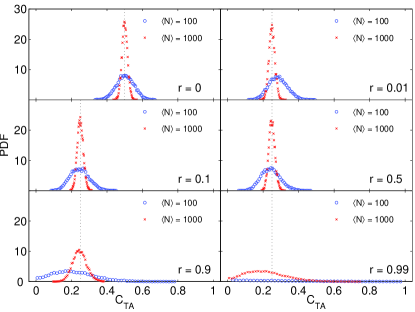
Figure 2: Distribution of time-averaged correlation function for $\psi(\tau)=e^{-\tau}$ is seen to approach the Dirac delta function as the average number of transitions per realization $\left\langle N\right\rangle$ grows. Location of the delta function shifts from $1/2$ for $r=0$ to $1/4$ for any $r\neq 0$ for large enough $T^{\prime}$(and hence also $t^{\prime}$), as indicated by the dotted line. Here $\left\langle N\right\rangle=T^{\prime}$.

The picture is completely different when we consider Eq. (1) with $\theta<1$, as is shown below. There is no narrowing of the distribution, and it actually tends to a universal shape, which is a function of r and $\theta$ alone. The analogue of this distribution in the ergodic case is the Dirac delta, Eq. (4). In the ergodic case, one is usually interested in the non-universal behavior for relatively short $t^{\prime}$ of the order of mean sojourn time, while for long $t^{\prime}$ the behavior is trivial. On the contrary, in the non-ergodic regime we consider, the behavior of interest in this paper is the universal nontrivial asymptotic behavior. From now on, $\theta<1$ 1<theta<2 .

II.2 Non-ergodic case

We begin the discussion of a non-ergodic situation by illustrating two randomly selected trajectories for $\theta=0.3$ in Fig. 3.

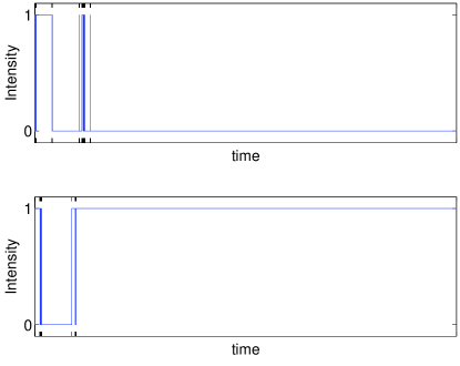
Figure 3: Two randomly selected trajectories for $\theta=0.3$. There are approximately 1000 transitions in each trajectory. The behavior is dominated by a few large intervals and hence is strongly nonergodic.

Clearly, these two trajectories are different, and hence time averaged correlation functions of these two trajectories will be different, yielding ergodicity breaking. It is important to emphasize that increasing the measurement time $T^{\prime}$, would not yield an ergodic behavior, since the process has no characteristic average time scale. In Fig. 4

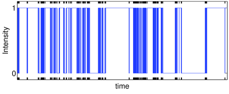
Figure 4: One randomly selected trajectory for $\theta=0.8$ with 1000 transitions. In comparison to $\theta=0.3$ (Fig. 3), the longest sojourn times here are shorter and the behavior is less nonergodic.

we show one trajectory with $\theta=0.8$ to compare to Fig. 3. One can say that for $\theta=0.8$ the nonergodicity is weaker. Unlike Fig. 3, in Fig. 4 we do not see one long on or off period dominating the time series. In Figure 5 we plot ten typical realizations of a correlation function, for a power-law decaying $\psi(\tau)$ following Eq. (1) with $\theta=0.3$ and $\theta=0.8$. The most striking feature of this figure is that the correlation functions are random. For very small r there is more or less smooth evolution of the correlation functions. As r grows their behavior becomes more chaotic.

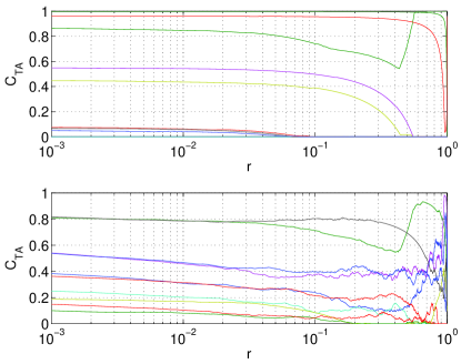
Figure 5: Ten typical realizations of $C_{TA}$ dependence on $r=t^{\prime}/T^{\prime}$ for $\theta=0.3$ (top) and $\theta=0.8$ (bottom). $T^{\prime}$ is kept constant, $t^{\prime}$ changes. For an ergodic process all correlation functions would follow the same master curve, the ensemble average correlation function.

We stress that this randomness is a true behavior and is not a problem in our simulations.

For many realizations, our numerical simulations are used to obtain $P_{C_{TA}(t^{\prime},T^{\prime})}(z)$ depicted in Figures 6

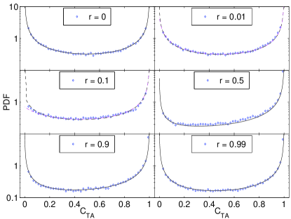
Figure 6: PDF of $C_{TA}(t^{\prime},T^{\prime})$ for different $r=t^{\prime}/T^{\prime}$ and $\theta=0.3$. $\left\langle N\right\rangle\approx 10^{3}$, $T^{\prime}\approx 1.66\times 10^{10}$. Abscissas are possible values of $C_{TA}(t^{\prime},T^{\prime})$. Diamonds are numerical simulations. Curves are analytical results without fitting: for $r=0$ Eq. (7) is used (full line), for $r=0.01$ and 0.1 Eq. (23) is used (dashed) and for $r=0.5$, 0.9 and 0.99 Eq. (29) is used (full). See Section VI for details.

, 7 and 8 for $\theta=0.3$, $\theta=0.5$ and $\theta=0.8$, respectively ($\left\langle N\right\rangle$ is the average number of transitions per realization; details of these simulations are deferred until Section VI and theoretical analysis is developed in Section V below). The diamonds are numerical results. In all the figures we vary $r\equiv t^{\prime}/T^{\prime}$. First consider the case $r=0$. For $\theta=0.3$ and $\theta=0.5$ we see from Figs. 6 and 7 that the PDF $P_{C_{TA}(t^{\prime},T^{\prime})}(z)$ has a $U$ shape. This is a strong non-ergodic behavior, since the PDF does not peak on the ensemble averaged value of the correlation function which is $1/2$. On the other hand, when $\theta=0.8$ the PDF $P_{C_{TA}(t^{\prime},T^{\prime})}(z)$ has a $W$ shape (cf. Fig. 8), a weak non ergodic behavior. To understand the origin of this type of transition note that as $\theta\rightarrow 0$ we expect the process to be in an on state or an off state for the whole duration of the measurement. This is so because the probability that the sojourn time is longer then $T^{\prime}$ will be $\sim(T^{\prime})^{-\theta}\rightarrow 1$ (cf. Fig. 3). Hence in that case the PDF of the correlation function will peak on $C_{TA}(t^{\prime},T^{\prime})=1$ and $C_{TA}(t^{\prime},T^{\prime})=0$ (i.e $U$ shape behavior). On the other hand when $\theta\rightarrow 1$ we expect a more ergodic behavior, since for $\theta>1$ the mean on and off periods are finite, this manifests itself in a peak of the distribution function of $C_{TA}(t^{\prime},T^{\prime})$ on the ensemble average value of $1/2$ and a $W$ shape PDF emerges (Fig 8, $r=0$). Note that for $\theta<1$ there is still statistical weight for trajectories which are on or off for periods of the order of the measurement time $T^{\prime}$, and the distribution of $C_{TA}(0,T^{\prime})$ attains its maximum on $C_{TA}(0,T^{\prime})=1$ and $C_{TA}(0,T^{\prime})=0$.

For $r>0$ we observe in Figs. 6 and 8 non-symmetrical and non-trivial shapes of the PDF of the correlation function. These PDFs agree very well with the analytical results, which we derive later. Not shown in Figs. 6, 7 and 8 is a delta function contribution on $C_{TA}(t^{\prime},T^{\prime})=0$. In other words, for $t^{\prime}\neq 0$, some of the random correlation functions are equal zero. The number of such correlation functions is increasing when r is increased. When $r\rightarrow 1$, half of the correlation functions are equal to zero (see Section V). Qualitatively, considering large r, the correlation is between the signal close to its starting point and the signal close to its end point. Roughly speaking, close to the end of the signal, typically long sojourn intervals with no transitions occur (cf. Fig. 3; i.e. persistence, as explained later in the paper in more detail - cf. Eq. (14)). For those types of trajectories being in state off at the end, the correlation function should be zero. We stress that the distributions observed on Figs. 6, 7 and 8 are not a scaling artifact: analogous calculations in the case of $\theta>1$ lead in the limit $T^{\prime}\rightarrow\infty$ to Dirac $\delta$-functions instead, as was shown above (Section II.1; cf. Fig. 2).

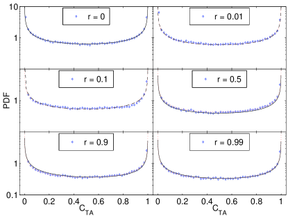
Figure 7: PDF of $C_{TA}(t^{\prime},T^{\prime})$ for different $r=t^{\prime}/T^{\prime}$ and $\theta=0.5$. $\left\langle N\right\rangle\approx 10^{3}$, $T^{\prime}\approx 2.47\times 10^{6}$. Diamonds are numerical simulations. Curves are analytical results without fitting: for $r=0$ Eq. (7) is used (full line), for $r=0.01$ and 0.1 Eq. (23) is used (dashed) and for $r=0.5$, 0.9 and 0.99 Eq. (29) is used (full). See Section VI for details.

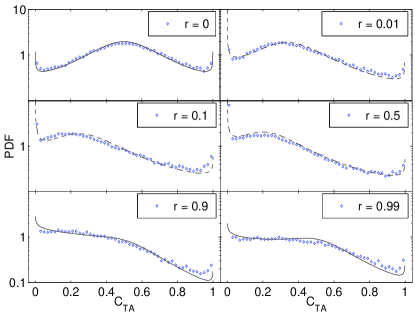
Figure 8: PDF of $C_{TA}(t^{\prime},T^{\prime})$ for different $r=t^{\prime}/T^{\prime}$ and $\theta=0.8$. $\left\langle N\right\rangle\approx 10^{4}$, $T^{\prime}\approx 6.15\times 10^{5}$. Diamonds are numerical simulations. Curves are analytical results without fitting: for $r=0$ Eq. (7) is used (full line), for $r=0.01$, 0.1 and 0.5 Eq. (23) is used (dashed) and for $r=0.9$ and 0.99 Eq. (29) is used (full). See Section VI for details.

We now turn to an analytical treatment of the described non-ergodicity.

III $t^{\prime}=0$: Lamperti distribution

In the case $t^{\prime}=0$ there exists known asymptotically exact expression for $P_{C_{TA}(0,T)}(z)$. Let us define

$$\mathcal{I}_{[a,b]}=\frac{\int_{a}^{b}I(t)\textrm{d}t}{b-a},$$ (5)

the time average intensity between time $a$ and time $b>a$. For $t^{\prime}=0$ from Eq. (2) it immediately follows that the time averaged correlation function is identical to the time average intensity

$$C_{TA}(0,T)=\mathcal{I}_{[0,T]}=\frac{T_{[0,T]}^{+}}{T}$$ (6)

where $T_{[a,b]}^{+}$ is the total time on of a particular realization in the time interval $[a,b]$. The time average intensity $\mathcal{I}_{[0,T]}$ has a known asymptotic distribution as $T\rightarrow\infty$, found originally by Lamperti Lamp ; GL and denoted in this paper as $\ell_{\theta}$:

$$P_{C_{TA}(0,T)}(z)=l_{\theta}\left(z\right),$$

and

$$l_{\theta}\left(z\right)=\frac{\sin\pi\theta}{\pi}\frac{z^{\theta-1}\left(1-z\right)^{\theta-1}}{z^{2\theta}+(1-z)^{2\theta}+2z^{\theta}\left(1-z\right)^{\theta}\cos\pi\theta},$$ (7)

for $0\leq z\leq 1$. For negative z and for $z>1$ it is zero. Note that $\ell_{\theta}(z)=\ell_{\theta}(1-z)$ and $\ell_{\theta}(z)$ diverges at $z=0,1$. This function is normalized to 1 for any $0<\theta\leq 1$. The Lamperti PDF is shown in Figs. 6, 7 and 8 for the case $r=0$, together with the numerical results. The transition between the $U$ shape behavior and the $W$ shape behavior happens at $\theta_{c}=0.5946...$. Lamperti distribution is related to the well known arcsine law Feller (case $\theta=1/2$). Other works regarding relative time spent by a system in one of two states are Bald ; Dhar ; BelBarkai .

IV Ensemble average $\left\langle C_{TA}(t^{\prime},T^{\prime})\right\rangle$

Another useful asymptotically exact result that can be derived is the mean of $P_{C_{TA}(t^{\prime},T^{\prime})}(z)$, i.e., the ensemble average of $C_{TA}(t^{\prime},T^{\prime})$. Generalizing to slightly different on and off time PDFs, with equal exponents but different coefficients,

$$\psi_{\pm}(t)\sim A_{\pm}t^{-1-\theta},$$ (8)

it has been shown MB_JCP that the mean intensity-intensity correlation function is asymptotically, for $t^{\prime}\geq 0$

$$\left\langle I(t)I(t+t^{\prime})\right\rangle\sim P_{+}-P_{+}P_{-}\frac{\sin\pi\theta}{\pi}B\left(\frac{1}{1+t/t^{\prime}};1-\theta,\theta\right),$$ (9)

where the incomplete beta function is defined as

$$B(z;\alpha,\beta)=\int_{0}^{z}x^{\alpha-1}(1-x)^{\beta-1}dx$$ (10)

and

$$P_{\pm}=\frac{A_{\pm}}{A_{+}+A_{-}}.$$

In the particular case of equal $\psi_{\pm}(t)$ we have $P_{\pm}=1/2$. Eq. (9) exhibits aging since the correlation function depends on t even when it is long. Aging of the ensemble average correlation function is related to nonergodicity of single realization trajectory.

Integrating we thus obtain from Eq. (2)

$$\begin{array}[]{c}\left\langle C_{TA}(t^{\prime},T^{\prime})\right\rangle={\displaystyle\frac{\int_{0}^{T}\left\langle I(t)I(t+t^{\prime})\right\rangle dt}{T}}\sim P_{+}^{2}+P_{+}P_{-}\times\\ \\ {\displaystyle\frac{\sin\pi\theta}{\pi}}\left[{\displaystyle\frac{B(1-r;\theta,1-\theta)}{1-r}-\frac{1}{\theta}\left(\frac{r}{1-r}\right)^{1-\theta}}\right].\end{array}$$ (11)

We see that the mean of the single trajectory correlation function asymptotically depends only on the ratio r of its arguments. We will show that the same is true also for the whole PDF of this random function, and not only for its mean. For r close to zero and to one,

$$\begin{array}[]{c}\left\langle C_{TA}(t^{\prime},T^{\prime})\right\rangle\sim\\ \\ \left[\begin{array}[]{cc}P_{+}\left(1-(1-P_{+}){\displaystyle\frac{r^{1-\theta}\sin\pi\theta}{\pi\theta(1-\theta)}}\right),&r\ll 1\\ \\ P_{+}^{2}+P_{+}P_{-}{\displaystyle\frac{(1-r)^{\theta}\sin\pi\theta}{\pi\theta(1+\theta)}},&1-r\ll 1.\end{array}\right.\end{array}$$ (12)

It is worth mentioning that for an ergodic time series the variance

$$\sigma_{\mathcal{I}}^{2}(T)=\left\langle\left(\mathcal{I}_{[0,T]}-\left\langle\mathcal{I}_{[0,T]}\right\rangle\right)^{2}\right\rangle=\left\langle\mathcal{I}_{[0,T]}^{2}\right\rangle-\left\langle\mathcal{I}_{[0,T]}\right\rangle^{2}$$

should go to zero as $T\rightarrow\infty$. In the case $\theta<1$, in this limit $\left\langle\mathcal{I}_{[0,T]}\right\rangle\rightarrow P_{+}$ MB_JCP and using Eq. (9),

$$\sigma_{\mathcal{I}}^{2}(T)\rightarrow\frac{\sin\pi\theta}{\pi}P_{+}P_{-}\int_{0}^{1}B(x;\theta,1-\theta)dx=P_{+}P_{-}(1-\theta),$$ (13)

which is non-zero, and so we can prove the non-ergodicity of the considered process, even without knowing $P_{C_{TA}(t^{\prime},T^{\prime})}(z)$. The last equality can be easily obtained using Eq. (10).

We conclude this section by introducing the probability $p_{0}(a,b)$ of making no transition, either up to down or vice versa, between two arbitrary times $a$ and $b\geq a$, known as the persistence probability. For large $a$ (cf. Eq. (44))

$$p_{0}(a,b)\sim\frac{\sin\pi\theta}{\pi}B\left(a/b;\theta,1-\theta\right).$$ (14)

Without going into details, we note that this probability plays important role in Lévy walks, and in particular in formulas given above GL ; MB_JCP . Its crucial feature is that it depends on the ratio of times and not on their difference, as is the case for ergodic processes. See also Dhar ; Majumdar .

Remark: Eq. (13) also follows from the fact that $\sigma_{\mathcal{I}}^{2}(T)$ should approach the variance of the Lamperti distribution (for $P_{+}=P_{-}$), whose moments can be calculated (GL, , appendix B).

V $t^{\prime}\neq 0$: Approximate solution

We were able to obtain only a formal exact solution for the PDF of $C_{TA}(t^{\prime},T^{\prime})$ for $t^{\prime}\neq 0$ (see Appendix A). Therefore, we resort to approximations. To start our analysis we divide the integration interval $[0,T]$ into sojourn times $\tau_{j}$. For convenience we redefine the first $t_{j}>T$ to be equal to $T$, and denote its index by n: $t_{n}\equiv T$. Accordingly, $\tau_{n}$ is redefined to be $T-t_{n-1}$ [cf. Fig. (1)]. Thus, for $i\leq n$ we write

$$C_{TA}(t^{\prime},T^{\prime})=\frac{\sum_{i\,\,\mbox{odd}}^{n}\int_{t_{i-1}}^{t_{i}}I(t+t^{\prime})\textrm{d}t}{T},$$ (15)

where we used the initial condition that $I(t)=1$ at time $t=0$. Hence $I(t)=1$ in $t_{i-1}<t<t_{i}$ when $i$ is odd, otherwise it is zero. The summation in Eq. (15) is over odd $i$’s, and $t_{n}=T$, namely $n-1$ in Eq. (15) is the random number of transitions in the interval $[0,T]$. From Eq. (15) we see that the time averaged correlation function, multiplied by T, is a sum of the random variables

$$\int_{t_{i-1}}^{t_{i}}I(t)I(t+t^{\prime})\textrm{d}t=\left\{\begin{array}[]{ll}\tau_{i}-t^{\prime}+\mathcal{I}_{[t_{i},t_{i}+t^{\prime}]}t^{\prime}&i\,\,\mbox{odd,}\,\,\tau_{i}>t^{\prime}\\ \mathcal{I}_{[t_{i-1}+t^{\prime},t_{i}+t^{\prime}]}\tau_{i}&i\,\,\mbox{odd,}\,\,\tau_{i}<t^{\prime}\\ 0&i\,\,\mbox{even}.\end{array}\right.$$ (16)

Using Eqs. (15, 16) we find an exact expression for the correlation function

$$\begin{array}[]{c}TC_{TA}\left(t^{\prime},T^{\prime}\right)={\displaystyle\sum_{i\,\,\mbox{odd}}^{n}}\tau_{i}-{\displaystyle\sum_{\begin{array}[]{c}i\,\,\mbox{odd}\\ \tau_{i}<t^{\prime}\end{array}}^{n}}(1-\mathcal{I}_{[t_{i-1}+t^{\prime},t_{i}+t^{\prime}]})\tau_{i}\\ -\,\,\,t^{\prime}{\displaystyle\sum_{\begin{array}[]{c}i\,\,\mbox{odd}\\ \tau_{i}>t^{\prime}\end{array}}^{n}}\left(1-\mathcal{I}_{[t_{i},t_{i}+t^{\prime}]}\right).\end{array}$$ (17)

The first term on the right hand side of this equation is $T^{+}$ the total time spent in state on in the time interval $[0,T]$, in the remaining two terms we have considered sojourn times $\tau_{i}$ larger or smaller than $t^{\prime}$ separately.

The core idea of our approximate solution is to replace the time-averaged intensities entering Eq. (17) by their mean-field value, specific for a given realization. Then for short $t^{\prime}$ we replace $\mathcal{I}_{[t_{i-1}+t^{\prime},t_{i}+t^{\prime}]}$ and $\mathcal{I}_{[t_{i},t_{i}+t^{\prime}]}$ by $\mathcal{I}_{[0,T]}$, while for long $t^{\prime}$ we use $\mathcal{I}_{[t^{\prime},T^{\prime}]}$ instead. Some alternative approximations are given in Appendix C. In the following, we treat short and long $t^{\prime}$ separately.

V.1 Small $t^{\prime}$

Within the mean field theory, Eq. (17) is approximated by

$$TC_{TA}(t^{\prime},T^{\prime})=\mathcal{I}_{[0,T]}T-\left(1-\mathcal{I}_{[0,T]}\right)\left(t^{\prime}N^{+}+\Sigma^{+}\right)$$ (18)

where $N^{+}$ is the number of odd (i.e. on) intervals satisfying $\tau_{i}\geq t^{\prime}$ and $i\leq n$, while $\Sigma^{+}\equiv\sum_{i\,\,\mbox{odd},\tau_{i}<t^{\prime}}^{n}\tau_{i}$ is the sum of all odd $\tau_{i}<t^{\prime}$ and $i\leq n$. For any particular realization $N^{+}$ will decrease with $t^{\prime}$ in a step-wise fashion, while $\Sigma^{+}$ will increase in a step-wise fashion. The term $t^{\prime}N^{+}+\Sigma^{+}$ in Eq. (18), however, will be continuous.

We proceed by replacing $N^{+}$ and $\Sigma^{+}$ with their scaling forms. $N^{+}$ should scale as $\sim n^{+}\int_{t^{\prime}}^{T^{+}}\psi(\tau)d\tau$ and $\Sigma^{+}\sim n^{+}\int_{0}^{t^{\prime}}\tau\psi(\tau)d\tau$, where $n^{+}$ is the number of on intervals comprising a given $T^{+}$. First note that for $t^{\prime}>T^{+}$, $N^{+}=0$ and $\Sigma^{+}=T^{+}$. Second, we assume

$$n^{+}\sim\frac{\sin\pi\theta}{\pi\theta}(T^{+})^{\theta}$$ (19)

in analogy to the scaling of n with T (e.g., GL ). Therefore, using Eq. (1) we propose that for $1\ll t^{\prime}\leq T^{+}$

$$N^{+}\approx\frac{\sin\pi\theta}{\pi\theta}\left[\left(\frac{T^{+}}{t^{\prime}}\right)^{\theta}-1\right],$$ (20)

and similarly,

$$\Sigma^{+}\approx t^{\prime}\left(\frac{T^{+}}{t^{\prime}}\right)^{\theta}.$$ (21)

Finally, plugging Eqs. (20, 21) into Eq. (18) results in

$$C_{TA}(t^{\prime},T^{\prime})\simeq\left\{\begin{array}[]{l l}{\mathcal{I}}_{[0,T]}\left\{1-\left(1-{\mathcal{I}}_{[0,T]}\right)\left[\left({r\over{(1-r)\mathcal{I}}_{[0,T]}}\right)^{1-\theta}\left({\sin\pi\theta\over\pi\theta}+1\right)-{\sin\pi\theta\over\pi\theta}{r\over{(1-r)\mathcal{I}}_{[0,T]}}\right]\right\}&\ t^{\prime}<T^{+}\\ {\mathcal{I}}_{[0,T]}^{2}&\ t^{\prime}>T^{+}.\end{array}\right.$$ (22)

Eq. (22) yields the correlation function, however unlike standard ergodic theories the correlation function here is a random function since it depends on $\mathcal{I}_{[0,T]}$.

The PDF of $C_{TA}(t^{\prime},T^{\prime})=z$ is now easy to find from the Lamperti PDF of $\mathcal{I}_{[0,T]}=x$. Using the chain rule, and Eqs. (6,7, 22):

$$P_{C_{TA}(t^{\prime},T^{\prime})}(z(x))\approx\frac{\ell_{\theta}(x)}{\left|{\displaystyle\frac{dz(x)}{dx}}\right|}$$ (23)

which is a parametric representation of $P_{C_{TA}(t^{\prime},T^{\prime})}(z)$ ($dz/dx=dC_{TA}(t^{\prime},T^{\prime})/d\mathcal{I}_{[0,T]}$ is found from Eq. (22)).

In Figs. 6, 7 and 8 we plot the PDF of $C_{TA}(t^{\prime},T^{\prime})$ (dashed curves) together with numerical simulations (diamonds) and find excellent agreement between theory and simulation, for the cases where our approximations are expected to hold $r<1/2$. In the above treatment we approximated $\mathcal{I}_{[t^{\prime},T^{\prime}]}$ by $\mathcal{I}_{[0,T]}$, which is legitimate only for small enough $t^{\prime}<T$, leading to a deterministic dependence of $C_{TA}(t^{\prime},T^{\prime})$ on $\mathcal{I}_{[0,T]}$.

Remark 1: Note that in the ergodic case (in which we can insert $\theta=1$ in the scaling relations) it follows that $C_{TA}(0,T^{\prime})=\mathcal{I}_{[0,T]}=1/2$ for $r=0$ and $C_{TA}(0,T^{\prime})=\mathcal{I}_{[0,T]}^{2}=1/4$ for any $r\neq 0$. This behavior reflects complete decorrelation of $I(t)$ and $I(t+t^{\prime})$ for any (large enough) $t^{\prime}$, irrespective of the value of $T^{\prime}$, as is indeed the case.

Remark 2: There is a certain similarity between Eq. (22) and Eq. (12) for small r. Only qualitatively, a realization with a given $\mathcal{I}_{[0,T]}$ can be viewed as generated using $\psi_{\pm}(\tau)$ with $A_{+}\neq A_{-}$ (cf. Eq. (8)), such that $P_{+}=\mathcal{I}_{[0,T]}$. See additional discussion of Eq. (22) in Appendix D.

V.2 Large $t^{\prime}$

To understand the behavior of the PDF of the correlation function for the limiting case $t^{\prime}\approx T^{\prime}\gg T$ the concept of persistence is important (see Eq. (14)). Recall that the probability of $I(t+t^{\prime})=const$ on the interval $[t^{\prime},T^{\prime}]$ grows to unity as $t^{\prime}/T^{\prime}\rightarrow 1$. Moreover, there is virtually no dependence on the signal values on $t\in[0,T]$ and thus

$$P_{C_{TA}(t^{\prime},T^{\prime})}(z)\approx\frac{1}{2}\ell_{\theta}(z)+\frac{1}{2}\delta(z-0).$$ (24)

There is a collapse of half of the trajectories to a $\delta$-peak at $z=0$, because of zero intensity of the signal on $[t^{\prime},T^{\prime}]$ in one of the two states, with probability $\rightarrow 1/2$. In the second case the signal will be unity throughout the interval $[t^{\prime},T^{\prime}]$, with probability $\rightarrow 1/2$, while its relative on time distribution in $[0,T]$ is given by Lamperti PDF.

More generally, for $t^{\prime}$ not so large, but still $t^{\prime}>T$ we use the mean-field, or decoupling approximation yielding from Eq. (17)

$$C_{TA}(t^{\prime},T^{\prime})\approx\mathcal{I}_{[0,T]}\mathcal{I}_{[t^{\prime},T^{\prime}]}.$$ (25)

To calculate the PDF of $C_{TA}(t^{\prime},T^{\prime})$ in Eq. (25) we use two steps: (i) calculate the PDF of $\mathcal{I}_{[t^{\prime},T^{\prime}]}=z$ which statistically depends on $\mathcal{I}_{[0,T]}$ (it is denoted as $P_{\mathcal{I}_{[t^{\prime},T^{\prime}]}}(z|\mathcal{I}_{[0,T]})$) and then (ii) using the distribution of $\mathcal{I}_{[0,T]}$, which is the Lamperti’s PDF Eq. (7), calculate the PDF of $C_{TA}(t^{\prime},T^{\prime})=z$:

$$P_{C_{TA}(t^{\prime},T^{\prime})}(z)\sim\int_{0}^{1}\ell_{\theta}(x)P_{\mathcal{I}_{[t^{\prime},T^{\prime}]}}\left(\left.\frac{z}{x}\right|x\right)\frac{dx}{x}.$$ (26)

Using the persistence probability Eq. (14), we approximate the conditional PDF of $\mathcal{I}_{[t^{\prime},T^{\prime}]}=z$ for a given $\mathcal{I}_{[0,T]}$ in the case $T\ll t^{\prime}$ by

$$P_{\mathcal{I}_{[t^{\prime},T^{\prime}]}}(z|\mathcal{I}_{[0,T]})\simeq\left[1-p_{0}\left(T,T^{\prime}\right)\right]Q_{\mathcal{I}_{[t^{\prime},T^{\prime}]}}\left(z\right)+p_{0}\left(T,T^{\prime}\right)\left[\mathcal{I}_{[0,T]}\delta\left(z-1\right)+\left(1-\mathcal{I}_{[0,T]}\right)\delta\left(z\right)\right],$$ (27)

where $Q_{\mathcal{I}_{[t^{\prime},T^{\prime}]}}\left(z\right)$ is the PDF of $\mathcal{I}_{[t^{\prime},T^{\prime}]}$ conditioned that at least one transition occurs in $[T,T^{\prime}]$. In Eq. (27) we introduced the correlation between $\mathcal{I}_{[t^{\prime},T^{\prime}]}$ and $\mathcal{I}_{[0,T]}$ through the dependence of the right hand side of the equation on $\mathcal{I}_{[0,T]}$. We assumed that in the case of no transitions in the time interval $[T,T^{\prime}]$, the probability of the interval $[t^{\prime},T^{\prime}]$ to be all the time either $on$ or $off$ (the only possible choices) is linearly proportional to the value of $\mathcal{I}_{[0,T]}$.

The persistence probability controls also the behavior of

$$Q_{\mathcal{I}_{[t^{\prime},T^{\prime}]}}\left(z\right)\simeq\left[1-p_{0}\left(t^{\prime},T^{\prime}\right)\right]\Theta\left(0<z<1\right)+p_{0}\left(t^{\prime},T^{\prime}\right)\frac{\delta\left(z\right)+\delta\left(z-1\right)}{2}.$$ (28)

We assumed that if a transition occurs in the interval $[t^{\prime},T^{\prime}]$ the distribution of $\mathcal{I}_{[t^{\prime},T^{\prime}]}$ is uniform [i.e., $\Theta\left(0<z<1\right)=1$ if the condition in the parenthesis is correct]. This is a crude approximation which is, however, reasonable for our purposes (however when $\theta$ approaches 1, this approximation does not work). The delta functions in Eq. (28) arise from two types of trajectories: If no transition occurs either $\mathcal{I}_{[t^{\prime},T^{\prime}]}=1$ (state $on$) or $\mathcal{I}_{[t^{\prime},T^{\prime}]}=0$ (state $off$) with equal probability. An asymptotically exact expression for $Q_{\mathcal{I}_{[t^{\prime},T^{\prime}]}}\left(z\right)$ is given by Eq. (45) in Appendix B; given the approximate nature of our derivations, however, we chose to use Eq. (28) because it is much simpler.

Finally, from Eqs. (27,28,26), and using $\delta(a/x)=x\delta(a)$ for $x>0$, we obtain after some algebra

$$\begin{array}[]{l l}P_{C_{TA}(t^{\prime},T^{\prime})}\left(z\right)\simeq\left[1-p_{0}\left(T,T^{\prime}\right)\right]\left\{\left[1-p_{0}\left(t^{\prime},T^{\prime}\right)\right]\int_{z}^{1}{l_{\theta}\left(x\right)\over x}{\textrm{d}}x+{p_{0}\left(t^{\prime},T^{\prime}\right)\over 2}\left[l_{\theta}\left(z\right)+\delta\left(z\right)\right]\right\}+p_{0}\left(T,T^{\prime}\right)\left[zl_{\theta}\left(z\right)+{\delta\left(z\right)\over 2}\right].\end{array}$$ (29)

Note that to derive Eq. (29) we used the fact that $\mathcal{I}_{[0,T]}$ and $\mathcal{I}_{[t^{\prime},T^{\prime}]}$ are correlated. In Figs. 6,7 and 8 we plot these PDFs of $C_{TA}(t^{\prime},T^{\prime})$ (solid curves) together with numerical simulations (diamonds) and find good agreement between theory and simulation, for the cases where these approximations are expected to hold, $r>1/2$. Eq. (24) is recovered from Eq. (29) in the limit of $t^{\prime}/T^{\prime}\rightarrow 1$.

VI Numerical simulations and comparison to approximations

We performed Monte Carlo simulations to generate distributions of the time averaged correlation function $C_{TA}(t^{\prime},T^{\prime})$ for different values of $r=t^{\prime}/T^{\prime}$ and with different $\theta$. Specifically, for each chosen $\theta$ the function

$$\psi(\tau)=\left[\begin{array}[]{cc}\theta\tau^{-1-\theta},&\tau\geq 1\\ \\ 0,&\tau<1\end{array}\right.$$

was used to generate random sojourn times until certain cumulative time $T^{\prime}\gg 1$. This constitutes a single realization. Tens of thousands of realizations were generated for each $\theta$.

For each realization, $C_{TA}(t^{\prime},T^{\prime})$ was calculated for different $t^{\prime}$ using Eqs. (2) and (36). To check whether the PDF of $C_{TA}(t^{\prime},T^{\prime})$ depends only on r we used different $T^{\prime}$. We also used the one-sided L$\grave{\textrm{e}}$vy PDF for $\psi(\tau)$ and found that our results do not depend on details of $\psi(\tau)$ besides the exponent $\theta$ of course. In addition, we calculated $\left\langle C_{TA}(t^{\prime},T^{\prime})\right\rangle$ from our simulations and compared it to the theoretical result Eq. (11). The agreement is excellent, as long as $T=T^{\prime}-t^{\prime}\gg 1$.

Some simulations are shown on Figures 6, 7 and 8 together with various theoretical approximations, for $\theta=0.3,0.5\textrm{ and }0.8$ respectively. $\left\langle N\right\rangle$ is the number of transitions made until time $T^{\prime}$, averaged over realizations. Diamonds are simulated data. Solid lines for $r=0$ are $\ell_{\theta}(z)$ where $0\leq z\leq 1$ are possible values of $C_{TA}(0,T^{\prime})$. Dashed and solid lines for $r\neq 0$ are Eqs. (23) and (29) for $r\leq 0.5$ and $r\geq 0.5$, respectively.

The discontinuity of the dashed lines, which can be noticed at small values of $C_{TA}(t^{\prime},T^{\prime})$ for $r=0.1$ is due to the discontinuity of the derivative in Eq. (23) at $\mathcal{I}_{[0,T]}=r/(1-r)$, when $C_{TA}(t^{\prime},T^{\prime})$ becomes equal to $\mathcal{I}_{[0,T]}^{2}=r^{2}/(1-r)^{2}$, which is very small for small r. Overall, however, Eq. (23) agrees with the shown simulations for $r<0.5$.

Approximation (29) works well for all $\theta$ values and $r>0.5$, for which it was designed, and it can be seen that as r grows toward 1, the asymptotic result Eq. (24) is approached. The assumption of uniform distribution of $\mathcal{I}_{[t^{\prime},T^{\prime}]}$ for values between 0 and 1, used in Eq. (28), is an oversimplification when $\theta=0.8$, which is partly responsible for slight discrepancies with the simulated data. Qualitatively, the PDF of $\mathcal{I}_{[t_{1},t_{2}]}$ is similar to $\ell_{\theta}(z)$ which starts growing a maximum at $z=0.5$ for approximately $\theta>0.6$ and so Eq. (28) is not very accurate for $\theta=0.8$. Also, here $T^{\prime}\approx 6\times 10^{5}$ is not very large and therefore the simulated distributions haven’t completely reached their asymptotic forms (e.g., observe slight shape differences between simulated data and theory for $r=0$).

Dot-dashed lines in Fig. 6 for $\theta=0.3$ are based on Eq. (48). They are shown only for $r<0.5$; this approximation works well in the limit of small $\theta$ and r.

Our simulations show that for $\theta=0.5$ the PDF of $C_{TA}(t^{\prime},T^{\prime})=z$ is closely approximated by $2\left\langle C_{TA}(t^{\prime},T^{\prime})\right\rangle\ell_{0.5}(z)+\left(1-2\left\langle C_{TA}(t^{\prime},T^{\prime})\right\rangle\right)\delta(z)$. Dotted lines in Fig. 7 are the nonsingular part of this expression, i.e., Lamperti distributions normalized by the relative mean. They are in good agreement with the data, and therefore are hardly visible. We have no explanation for this fact, besides the qualitative argument that as r grows from zero, for lower $\theta$ the left side of the distribution drops (cf. Fig. 6), while for higher $\theta$ it rises (cf. Fig. 8), and so somewhere between $\theta=0.3$ and $\theta=0.8$ it might remain unchanged. For $t^{\prime}/T^{\prime}\rightarrow 1$ this expression approaches Eq. (24).

For $r=0$ the PDF of $C_{TA}(t^{\prime},T^{\prime})$ is the Lamperti distribution. As can be observed from comparison of the PDFs with $r=0$ and $r>0$ in Figs. 6 and 8, the PDF of $C_{TA}(t^{\prime},T^{\prime})$ is shifted to the left as r increases from zero. This is so because small $\mathcal{I}_{[0,T]}$ values mean small proportion of time spent on, and there is a large probability that a small $t^{\prime}$ will yield zero correlation in such realizations. This is in agreement with Eq. (48). For larger $\theta$ values, there are more short and less long intervals covering the time of  “experiment” $T^{\prime}$ (as can be seen from Eq. (47), because $r^{1-\theta}$ increases toward 1 with growing $\theta$, for any fixed $r>0$). Therefore, relatively small shift $t^{\prime}$ (small r) will cause no significant effect in the case of small $\theta$, dominated by large intervals, while in the case of large $\theta$ this small shift $t^{\prime}$ will decorrelate many intervals, thus significantly reducing the correlation function. Realizations with small $\mathcal{I}_{[0,T]}$ also will lose correlation faster for the same reason, leading to a non-uniform visible deformation of the shape of the PDF of $C_{TA}(t^{\prime},T^{\prime})$. Of course, as r grows this simple picture breaks. However, for r approaching unity we recover another simple asymptotic result (24).

VI.1 2D histograms

Two dimensional histograms, showing the frequency of events $C_{TA}(t^{\prime},T^{\prime})$ for a particular value of $\mathcal{I}_{[0,T^{\prime}]}$ are now considered. These histograms show the correlation between $C_{TA}(t^{\prime},T^{\prime})$ and $\mathcal{I}_{[0,T^{\prime}]}$. As we explained already for $r=0$ we have $C_{TA}(t^{\prime},T^{\prime})=\mathcal{I}_{[0,T^{\prime}]}$, hence we have total correlation in this simple case. When r is small, our approximate solution Eq. (22) suggests a strong correlation between $C_{TA}(t^{\prime},T^{\prime})$ and $\mathcal{I}_{[0,T^{\prime}]}$. However, the arguments we used to derive Eq. (22) neglect fluctuations since they are based on our non-ergodic mean field approximation. To check our mean field, and to understand its limitations, the two dimensional histograms we consider in this section are very useful. In addition, for large r we see from Eq. (29), that according to the decoupling approximation, the correlation between $C_{TA}(t^{\prime},T^{\prime})$ and $\mathcal{I}_{[0,T^{\prime}]}$ is expected to be weak, as is demonstrated indeed by correlation plots in Fig.

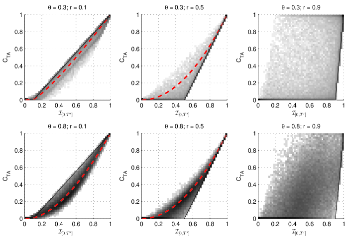
Figure 9: Distribution of $C_{TA}(t^{\prime},T^{\prime})$ as a function of $\mathcal{I}_{[0,T^{\prime}]}$ for different values of r and $\theta$. The gray scale is changed logarithmically with the number of occurrences inside a square bin. Darker regions mean higher occurrences. Dashed lines are Eq. (22) with $\mathcal{I}_{[0,T^{\prime}]}$ used instead of $\mathcal{I}_{[0,T]}$. Full lines $C_{TA}(t^{\prime},T^{\prime})=\left(\mathcal{I}_{[0,T^{\prime}]}-r\right)/(1-r)$ are shown as well.

9.

Leaving the details to Appendix E, we can derive the following rigorous boundaries (i.e., the inf and the sup) of $C_{TA}(t^{\prime},T^{\prime})$: for $r\geq 1/2$

$$\max\left\{0,\frac{\mathcal{I}_{[0,T^{\prime}]}-r}{1-r}\right\}\leq C_{TA}(t^{\prime},T^{\prime})\leq\min\left\{1,\frac{\mathcal{I}_{[0,T^{\prime}]}}{2(1-r)}\right\},$$ (30)

which is in agreement with Fig. 9. For $1/3\leq r<1/2$ we obtain

$$\begin{array}[]{c}\max\left\{0,\frac{\mathcal{I}_{[0,T^{\prime}]}+r-1}{1-r},\frac{2\mathcal{I}_{[0,T^{\prime}]}-r-1}{1-r}\right\}\leq C_{TA}(t^{\prime},T^{\prime})\\ \leq\min\left\{\frac{2\mathcal{I}_{[0,T^{\prime}]}}{3(1-r)},\frac{\mathcal{I}_{[0,T^{\prime}]}+1-2r}{2(1-r)}\right\}.\end{array}$$ (31)

For small r, on one hand the matters become more complicated, so our argument is more qualitative . First notice that if $T_{[0,T^{\prime}]}^{-}\equiv T^{\prime}-T_{[0,T^{\prime}]}^{+}$ is small enough then all the off intervals can lie inside $[t^{\prime},T]$ and be used twice (once in $I(t)$ and once in $I(t+t^{\prime})$, for $r\neq 0$) to multiply on intervals, hence $C_{TA}(t^{\prime},T^{\prime})\geq\left(T-2T_{[0,T^{\prime}]}^{-}\right)/T=\left(2\mathcal{I}_{[0,T^{\prime}]}-r-1\right)/(1-r)$. In most cases, small $T_{[0,T^{\prime}]}^{-}$ means that the last sojourn interval (going up to time $T^{\prime}$) is in state on and all the off intervals are inside $[0,T]$, so that $C_{TA}(t^{\prime},T^{\prime})\leq\left(T-T_{[0,T^{\prime}]}^{-}\right)/T=\left(\mathcal{I}_{[0,T^{\prime}]}-r\right)/(1-r)$. Compare this to Eq. (48) derived in Appendix C. It is argued there that this value of $C_{TA}(t^{\prime},T^{\prime})$ will be achieved more often for lower $\theta$, in agreement with Fig. 9. This is not a rigorous upper bound, though; see Appendix E. If $T_{[0,T^{\prime}]}^{+}$ is small enough then the lower bound will be zero. The sufficient (but not necessary, in general) condition to achieve zero is $T_{[0,T^{\prime}]}^{+}\leq 1/2$ as then we can construct a trajectory by choosing zero intensity at the time $t+t^{\prime}$ if it is 1 at time t, and vice versa.

On the other hand, for very small r (but $t^{\prime}$ can be large) we know that $C_{TA}(t^{\prime},T^{\prime})$ is almost unchanged, as the whole signal is dominated by relatively few largest sojourn intervals (cf. Eq. (47)); hence $C_{TA}(t^{\prime},T^{\prime})$ will be close to $\mathcal{I}_{[0,T^{\prime}]}$. The rigorous bounds are, therefore, hardly reached.

Remark: Our approximation Eq. (22), with $\mathcal{I}_{[0,T]}$ replaced by $\mathcal{I}_{[0,T^{\prime}]}$, is shown by the dashed lines on Fig. 9. For $r=1/2$ it actually reduces to $C_{TA}(t^{\prime},T^{\prime})=\mathcal{I}_{[0,T^{\prime}]}^{2}$, which works better for higher $\theta$, when the non-ergodicity is weaker. In fact, a more precise way to find $C_{TA}(t^{\prime},T^{\prime})$ in this case is using Eq. (25), but then there is no simple formula connecting $C_{TA}(t^{\prime},T^{\prime})$ and $\mathcal{I}_{[0,T]}$ like Eq. (22).

VI.2 Power spectrum

It is useful to look at power spectra (PS) of generated intensity signals Pelton04 ; Davidsen ; Zumofen93 ; Schriefl05 . Power spectrum is defined as

$$S(\omega)=\frac{\tilde{I}(\omega)\tilde{I}(-\omega)}{T^{\prime}},$$ (32)

where $\tilde{I}(\omega)$ is Fourier transform of $I(t)$ (cf. Eq. (39)). We calculate such PS and find, as expected, that they too exhibit a nonergodic behavior, as shown in Fig. 10. Each PS is random and does not fall on the ensemble averaged curve (dashed line) even after averaging the data in large frequency windows. Note that for smaller $\theta$ the PS values for a given $\omega$ are spread wider, which is a reflection of a wider distributions of correlation functions (cf. Figs. 6, 8). In light of the scaling $C_{TA}(t^{\prime},T^{\prime})\sim A-Br^{1-\theta}$ in expressions (12) and (22) for small enough r (but for $t^{\prime}$ as large as desired, as long as $T^{\prime}$ is large enough) we can argue that the PS will scale as (cf. Eq. (42))

$$\begin{array}[]{ccc}S(\omega)&\sim&-2B(T^{\prime})^{\theta-1}\textrm{Re}\int_{0}^{T^{\prime}}(t^{\prime})^{1-\theta}e^{-i\omega t^{\prime}}dt^{\prime}\\ &\approx&2BT^{\prime}\cos(\pi\theta/2)\Gamma(2-\theta)(\omega T^{\prime})^{\theta-2}\propto\omega^{\theta-2}\end{array}$$ (33)

as long as $\omega\gg 1/T^{\prime}$ (term A in $C_{TA}(t^{\prime},T^{\prime})$ leads to a term $2AT^{\prime}\sin\omega T^{\prime}/(\omega T^{\prime})$ which is zero for all $\omega\neq 0$ used in calculating discrete power spectrum). This is indeed the case, as illustrated in Fig. 10. In Eq. (33) we estimated the PS by Fourier transforming the correlation function, implying the well-known Wiener-Khintchine theorem. This theorem, however, is assumed valid only for stationary processes and for ensemble averaged correlation functions and spectra. Nevertheless, one can say that with respect to short sojourn times each realization is identical, and the observed non-ergodicity is due to necessarily poor statistics of long intervals (leading, in particular, to different values of B for different realizations). See Appendix A for discussion on a generalized Wiener-Khintchine theorem.

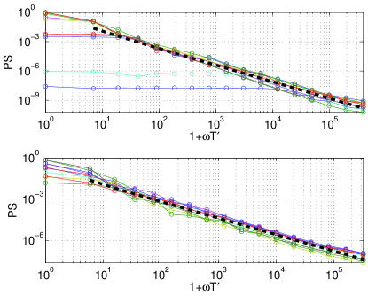
Figure 10: Power spectrum $S(\omega)/T^{\prime}$ for ten typical realizations shown in Fig. 5, for $\theta=0.3$ (top) and $\theta=0.8$ (bottom). Data for each realization are averaged in exponentially increasing with $\omega$ bins. Each curve is normalized in such a way that at $\omega=0$ the PS equals $\mathcal{I}_{[0,T^{\prime}]}^{2}$. The PS is random due to non-ergodicity of underlying process. Dashed lines are given by Eq. (34) and scale as $\omega^{\theta-2}$. The abscissas are $1+\omega T^{\prime}$ in order to show the value of PS at zero frequency on a log-log plot.

For the ensemble-averaged spectrum, using the value $B=\sin(\pi\theta)/(4\pi\theta(1-\theta))$ from Eq. (12),

$$\frac{\left\langle S(\omega)\right\rangle}{T^{\prime}}\sim\frac{\cos(\pi\theta/2)}{2\Gamma(1+\theta)}(\omega T^{\prime})^{\theta-2},\,\,\,\omega T^{\prime}\gg 1.$$ (34)

This line is also shown in Fig. 10.

VII Summary

We investigated autocorrelation of a dichotomous random process governed by identical waiting time distributions of its two states, characterized by zero and nonzero intensity. We considered the case of a power law waiting time with exponent $\theta$ lying between 0 and 1, as this choice is of considerable practical interest. This process is a one-dimensional Lévy walk process. Such power law distributions are experimentally observed, as discussed in the Introduction. These distributions lead to aging and non-ergodicity and in particular, to a distribution of possible values of a single trajectory two-time correlation function for fixed times, even in the limit when these times go to infinity. This is in striking contrast to the standard situation in which correlation function asymptotically assumes only one possible value for fixed times, equal to the ensemble average (ergodicity).

For our theoretical analysis of distributions of correlation functions we used the non-ergodic mean-field and the decoupling approximation, Eqs. (18) and (25), in which various temporal averages of the intensity were replaced by the total time averaged intensity $\mathcal{I}_{[0,T]}$ or $\mathcal{I}_{[t^{\prime},T^{\prime}]}$, specific for each realization. We then expressed the correlation function as a (deterministic or random) function of this time average. This enabled us to derive approximate results for the distributions of correlation functions from known distributions of time averaged intensity. We also related power spectra of single trajectories to the time averaged correlation functions, and demonstrated their nonergodicity as well as universal scaling which is a function of the exponent $\theta$ only. Our results agree well with numerical simulations, and, importantly, clarify the nature of the investigated non-ergodicity. Generalizations of our approach to situations with different on and off time distributions are possible.

In the context of blinking nanocrystals, we showed MB_JCP that the exponent $\theta=1/2$ is a result of a simple model of first passage time of charge carrier in three dimensions, based on standard diffusion. The experiments Dahan ; Zumofen04 ; Xie ; Weitz ; Kuno show, that rather generally, power law sojourn times describe dynamics of single particles in diverse systems. Since power law sojourn times (not necessarily for a two state process) lead to non-ergodic behavior, we expect that stochastic theories of ergodicity breaking will play an increasingly important role in the analysis of single particle experiments.

Appendix A Formal solution

We express the numerator in Eq. (2) through the cumulative renewal (transition) times $t_{j}$ by noting that $I(t)=const$ on intervals $t_{n}<t<t_{n+1}$, while $I(t+t^{\prime})=const$ on intervals $t_{m}-t^{\prime}<t<t_{m+1}-t^{\prime}$ and keeping in mind the restriction $0<t<T$. For convenience, we redefine the first $t_{j}$ which is $>T^{\prime}$ to be equal to $T^{\prime}$. The index of this $t_{j}$ is denoted by $N$. Note that $\tau_{N}\equiv T^{\prime}-t_{N-1}$ is not distributed according to $\psi(\tau)$. The temporal durations (lengths) of intervals where both $I(t)$ and $I(t+t^{\prime})$ are constant, are then

$$l_{mn}(t^{\prime})=\max\left\{0,\min(t_{n+1},t_{m+1}-t^{\prime})-\max(t_{n},t_{m}-t^{\prime})\right\}$$ (35)

and in particular

$$l_{nn}=\max\left\{0,\tau_{n+1}-t^{\prime}\right\}.$$

Obviously, $l_{m<n,n}=0$ and hence

$$\int_{0}^{T^{\prime}-t^{\prime}}I(t)I(t+t^{\prime})dt=\sum_{\begin{array}[]{c}n=0,\\ n\,\textrm{even}\end{array}}^{N-1}\sum_{\begin{array}[]{c}m=n,\\ m\,\textrm{even}\end{array}}^{N-1}l_{mn}.$$ (36)

Here, and throughout the article, we assume that the process starts in state on. This assumption is clearly asymptotically negligible, and is made here simply for purposes of notation.

Using the cumulative PDF of $\{\tau_{1},...,\tau_{N-1}\}$ and $N-1$ under the constraint $t_{N-1}<T^{\prime}$ GL (and because $\textrm{Prob}[t_{N-1}=T^{\prime}]=0$) we can write formally the PDF of $TC_{TA}(t^{\prime},T^{\prime})=x$ as

$$\begin{array}[]{c}f_{TC_{TA}(t^{\prime},T^{\prime})}(x)={\displaystyle\sum_{N=1}^{\infty}}\left({\displaystyle\prod_{k=1}^{N-1}}{\displaystyle\int_{0}^{\infty}}\psi(\tau_{k})d\tau_{k}\right)\mathcal{P}(t_{N}=T^{\prime})\times\\ \\ \times\Theta(T^{\prime}-t_{N-1})\delta\left(x-{\displaystyle\sum_{\begin{array}[]{c}n=0,\\ n\,\textrm{even}\end{array}}^{N-1}\sum_{\begin{array}[]{c}m=n,\\ m\,\textrm{even}\end{array}}^{N-1}}l_{mn}(t^{\prime})\right),\end{array}$$

where $\Theta$ is Heaviside step function, $\mathcal{P}(t_{N}=T^{\prime})$ is the probability that no transition occurred between $t_{N-1}$ and $T^{\prime}$, and $\delta$ is the Dirac delta.

In order to get rid of the max and min functions in Eq. (35), one can perform Laplace transform of Eq. (35) with respect to $t^{\prime}$ ($t^{\prime}\rightarrow u$) and write similar expression for the PDF of $T\hat{C}_{TA}(u,T^{\prime})$ (for real u). It can be shown that

$$\hat{l}_{m>n,n}(u)=\frac{e^{-u(t_{m+1}-t_{n})}(e^{u\tau_{m+1}}-1)(e^{u\tau_{n+1}}-1)}{u^{2}}$$ (37)

and

$$\hat{l}_{nn}(u)=\frac{u\tau_{n+1}-1+e^{-u\tau_{n+1}}}{u^{2}}.$$ (38)

We could not, unfortunately, utilize these expressions to calculate $f_{TC_{TA}(t^{\prime},T^{\prime})}(x)$ or $f_{T\hat{C}_{TA}(u,T^{\prime})}(x)$ and therefore have to resort to various approximations.

Relation to power spectrum

We derive a generalized form of Wiener-Khinchine theorem for nonergodic nonstationary processes. In analogy to the numerical spectral analysis of a time series, we assume here that the intensity signal is identically zero outside of the interval $[0,T^{\prime}]$. Then the Fourier transform of intensity is defined as

$$\tilde{I}(\omega)={\displaystyle\int_{-\infty}^{\infty}}I(t)e^{-i\omega t}dt={\displaystyle\int_{0}^{T^{\prime}}}I(t)e^{-i\omega t}dt$$ (39)

and the power spectrum of a realization is defined in Eq. (32). From Eqs. (39) and (32)

$$T^{\prime}S(\omega)={\displaystyle\int_{0}^{T^{\prime}}}I(t_{1})e^{-i\omega t_{1}}dt_{1}{\displaystyle\int_{0}^{T^{\prime}}}I(t_{2})e^{i\omega t_{2}}dt_{2}.$$

We now divide the integration over $t_{2}$ into two parts and replace the order of integration in the first part:

$$\begin{array}[]{ccc}{\displaystyle\int_{0}^{T^{\prime}}}dt_{1}{\displaystyle\int_{0}^{T^{\prime}}}dt_{2}&=&{\displaystyle\int_{0}^{T^{\prime}}}dt_{1}{\displaystyle\int_{0}^{t_{1}}}dt_{2}+{\displaystyle\int_{0}^{T^{\prime}}}dt_{1}{\displaystyle\int_{t_{1}}^{T^{\prime}}}dt_{2}\\ \\ &=&{\displaystyle\int_{0}^{T^{\prime}}}dt_{2}{\displaystyle\int_{t_{2}}^{T^{\prime}}}dt_{1}+{\displaystyle\int_{0}^{T^{\prime}}}dt_{1}{\displaystyle\int_{t_{1}}^{T^{\prime}}}dt_{2}.\end{array}$$

Swapping names $t_{1}$ and $t_{2}$ in the first part thus yields

$$T^{\prime}S(\omega)={\displaystyle\int_{0}^{T^{\prime}}}dt_{1}{\displaystyle\int_{t_{1}}^{T^{\prime}}}dt_{2}I(t_{1})I(t_{2})[e^{i\omega(t_{1}-t_{2})}+e^{i\omega(t_{2}-t_{1})}]$$

and introducing $t=t_{1}$ and $t^{\prime}=t_{2}-t_{1}$ results in

$$S(\omega)=\frac{1}{T^{\prime}}{\displaystyle\int_{0}^{T^{\prime}}}dt{\displaystyle\int_{0}^{T^{\prime}-t}}dt^{\prime}I(t)I(t+t^{\prime})[e^{-i\omega t^{\prime}}+e^{i\omega t^{\prime}}].$$

In a similar fashion, we can write the Laplace transform of

$$K(t^{\prime},T^{\prime})\equiv(T^{\prime}-t^{\prime})C_{TA}(t^{\prime},T^{\prime})={\displaystyle\int_{0}^{T^{\prime}-t^{\prime}}}dtI(t)I(t+t^{\prime})$$ (40)

with respect to $t^{\prime}$ as

$$\begin{array}[]{ccc}\hat{K}(u,T^{\prime})&=&{\displaystyle\int_{0}^{\infty}}dt^{\prime}e^{-ut^{\prime}}{\displaystyle\int_{0}^{T^{\prime}-t^{\prime}}}dtI(t)I(t+t^{\prime})\\ \\ &=&{\displaystyle\int_{0}^{T^{\prime}}}dt{\displaystyle\int_{0}^{T^{\prime}-t}}dt^{\prime}I(t)I(t+t^{\prime})e^{-ut^{\prime}}\end{array}$$

and it becomes evident that

$$T^{\prime}S(\omega)=\hat{K}(i\omega,T^{\prime})+\hat{K}(-i\omega,T^{\prime}).$$ (41)

This is a generalization of the Wiener-Khintchine theorem stating that the power spectrum is given by cosine Fourier transform of a correlation function. But while this theorem is used for ensemble-averaged correlation functions of stationary processes, here we have a similar relation for a non-stationary process, and without ensemble averaging. Note that the dependence on $T^{\prime}$ is preserved, in contrast to the regular Wiener-Khintchine theorem.

From Eq. (40) it follows that

$$\hat{K}(u,T^{\prime})=T^{\prime}\hat{C}_{TA}(u,T^{\prime})+\frac{\partial\hat{C}_{TA}(u,T^{\prime})}{\partial u}$$

and for large $uT^{\prime}\gg 1$, $\hat{C}_{TA}(u,T^{\prime})\approx\hat{K}(u,T^{\prime})/T^{\prime}$, leading finally to

$$\begin{array}[]{ccc}S(\omega)&=&\hat{C}_{TA}(i\omega,T^{\prime})+\hat{C}_{TA}(-i\omega,T^{\prime})\\ \\ &+&{\displaystyle\frac{\partial[\hat{C}_{TA}(i\omega,T^{\prime})-\hat{C}_{TA}(-i\omega,T^{\prime})]}{i\partial\omega}}\\ \\ &\approx&\hat{C}_{TA}(i\omega,T^{\prime})+\hat{C}_{TA}(-i\omega,T^{\prime})\end{array}$$ (42)

for large $\omega T^{\prime}\gg 1$. Note that for a single trajectory correlation defined as $\left(\int_{0}^{T^{\prime}-t^{\prime}}I(t)I(t+t^{\prime})dt\right)/T^{\prime}$ instead of Eq. (2) the generalized Wiener-Khintchine relation is exact for any $\omega$ (cf. Eq. (41)).

As an illustration, consider now our case of the on-off process. Fourier transform of an intensity $I(t)$ for a realization is:

$$\tilde{I}(\omega)={\displaystyle\frac{1}{-i\omega}\sum_{\begin{array}[]{c}n=0,\\ n\textrm{ even}\end{array}}^{N-1}}e^{-i\omega t_{n+1}}(1-e^{i\omega\tau_{n+1}}).$$

Then it is straightforward to show that

$$T^{\prime}S(\omega)=\hat{K}(i\omega,T^{\prime})+\hat{K}(-i\omega,T^{\prime}),$$

where $\hat{K}(u,T^{\prime})$ can be found utilizing Eqs. (36), (37) and (38). This is a particular case of the general relation (41).

Appendix B Distribution of $T_{[a,b]}^{+}$

Here we present asymptotically exact formula for a distribution of on times on an arbitrary interval $[a,b]$, where $a$ and $b-a$ are large enough. We denote the first renewal time after $a$ by $\nu$. We have to take two possibilities into account. First is that there was at least one renewal inside the interval and then $a<\nu<b$. Thus

$$T_{[a,b]}^{+}=Y+T_{[\nu,b]}^{+}$$

where Y is the on time from $a$ till first renewal $\nu$. Asymptotically, Y is independent of initial conditions and its PDF is

$$f_{Y}(y)=\frac{1}{2}\delta(y-(\nu-a))+\frac{1}{2}\delta(y-0),$$

where the two Dirac deltas correspond to being in state on or off.

After renewal at time $\nu$, again asymptotically, we can use the PDF of $T_{[\nu,b]}^{+}$ which is also independent of its “initial condition”, i.e., the value of Y being 0 or 1. Then the PDF of $T_{[\nu,b]}^{+}/(b-\nu)$ is given by the Lamperti $\ell_{\theta}$ and therefore for any fixed $\nu$

$$\begin{array}[]{c}f_{T_{[a,b]}^{+}}(x|\nu;\nu<b)\\ \\ =\frac{1}{2(b-\nu)}\left[\ell_{\theta}\left(\frac{x-(\nu-a)}{b-\nu}\right)+\ell_{\theta}\left(\frac{x}{b-\nu}\right)\right].\end{array}$$ (43)

The second possibility is that $\nu>b$ and in this case, clearly,

$$f_{T_{[a,b]}^{+}}(x|\nu;\nu>b)=\frac{1}{2}\delta(x-(b-a))+\frac{1}{2}\delta(x-0).$$

Introducing the PDF of the forward recurrence time, $f_{E}(\nu-a;a)$, which is the PDF of having to wait for the first renewal after time $a$ for a period of time $\nu-a$ GL , we finally obtain

$$\begin{array}[]{c}f_{T_{[a,b]}^{+}}(x)={\displaystyle\int_{a}^{b}}f_{T_{[a,b]}^{+}}(x|\nu)f_{E}(\nu-a;a)d\nu\\ \\ +\frac{1}{2}\left(\delta(x-(b-a))+\delta(x-0)\right){\displaystyle\int_{b}^{\infty}}f_{E}(\nu-a;a)d\nu,\end{array}$$

with $f_{T_{[a,b]}^{+}}(x|\nu)$ in the first integral given by Eq. (43). The last integral

$$p_{0}(a,b)={\displaystyle\int_{b}^{\infty}}f_{E}(\nu-a;a)d\nu$$ (44)

defines the persistence probability $p_{0}(a,b)$, for $b\geq a$. The function $f_{E}(\nu-a;a)$ is equal to $\psi(\nu)$ for $a=0$. For large $a$, it is the Dynkin function GL ; Feller ; MB_JCP

$$f_{E}(\nu-a;a)\sim\frac{\sin\pi\theta}{\pi}\frac{1}{\left(\frac{\nu}{a}-1\right)^{\theta}\nu},$$

and then $p_{0}(a,b)$ can be written as in Eq. (14).

Finally, the PDF of $\mathcal{I}_{[a,b]}=z$ is

$$Q_{\mathcal{I}_{[a,b]}}(z)=(b-a)f_{T_{[a,b]}^{+}}((b-a)z).$$ (45)

Appendix C Particular solutions

We consider here two situations which can be analyzed differently from the approach presented in Section V. This analysis helps understanding the structure of the correlation functions.

C.1 Extremely small $t^{\prime}$

If $t^{\prime}<\tau_{i},\,\,i=1,...,N$ then, using Appendix A, we obtain $l_{m>n+1,n}=0$, $l_{nn}=\tau_{n+1}-t^{\prime}$ and

$$TC_{TA}(t^{\prime},T^{\prime})=T_{[0,T^{\prime}]}^{+}-\left[\frac{N+1}{2}\right]_{int}t^{\prime}\approx T_{[0,T^{\prime}]}^{+}-\frac{Nt^{\prime}}{2}$$ (46)

where the subscript int indicates that […] denote integer part. It is easy to see that in this case, $T_{[0,T^{\prime}]}^{+}>0$ for $t^{\prime}>0$ and, moreover, $0<TC_{TA}(t^{\prime},T^{\prime})\leq T$, as it should (because $N\geq 1$).

The fraction of time $T^{\prime}$ covered by short intervals $\tau_{i}<t^{\prime}$ scales as

$$\frac{\int_{0}^{t^{\prime}}t\psi(t)dt}{\int_{0}^{T^{\prime}}t\psi(t)dt}\approx\left(\frac{t^{\prime}}{T^{\prime}}\right)^{1-\theta}=r^{1-\theta}$$ (47)

for large enough $t^{\prime}$ and $T^{\prime}$. Hence the contribution of these short intervals is negligible if $t^{\prime}\ll T^{\prime}$, although $t^{\prime}$ is large (in contrast to the case when the mean sojourn time is finite and the fraction of time covered by intervals shorter than $t^{\prime}$ grows to 1 as $t^{\prime}$ increases, irrespective of the ratio $t^{\prime}/T^{\prime}$). Therefore, we argue that Eq. (46) can still be used when $t^{\prime}\ll T^{\prime}$, if by $N$ we understand the number $N_{eff}$ of intervals longer than $t^{\prime}$. It is important, however, to distinguish these coarsened intervals from the original intervals $\tau_{i}$. The durations $\tau_{eff}$ of the coarsened intervals are not governed by $\psi(\tau)$. For a power law $\psi(\tau)$ we expect that their durations are still governed by a power law PDF with the same exponent $\theta$. Nevertheless, it is questionable to use asymptotic expressions for $N_{eff}$ as a function of $t^{\prime}/T^{\prime}$, constructed in a fashion used in Section V, because the PDF of $\tau_{eff}$ does not have to be a power law for $\tau_{eff}\sim t^{\prime}$ (and it is zero for $\tau_{eff}<t^{\prime}$).

C.2 Small $\theta$ and intermediate $t^{\prime}$

It is possible to make an exact calculation if there exists an interval number k, and for $t^{\prime}$ such that

$$\sum_{\begin{array}[]{c}i=1\\ i\neq k\end{array}}^{N}\tau_{i}<t^{\prime}<\tau_{k}.$$

Ubiquitous realization of this condition could be expected for small $\theta$, when the longest interval often approaches the “experimental” time $T^{\prime}$. Then, for $m>n$ using

$$\begin{array}[]{ccc}t_{n}-(t_{m}-t^{\prime})&=&t^{\prime}-{\displaystyle\sum_{i=n+1}^{m}}\tau_{i}\\ \\ t_{n+1}-(t_{m+1}-t^{\prime})&=&t^{\prime}-{\displaystyle\sum_{i=n+2}^{m+1}}\tau_{i}\end{array}$$

yields

$$l_{m>n+1,n}=\delta_{n,k-1}\tau_{m+1}+\delta_{m,k-1}\tau_{n+1};$$

also

$$l_{nn}=\delta_{n,k-1}(\tau_{k}-t^{\prime}),$$

where $\delta_{ij}$ is Kronecker delta, and hence

$$C_{TA}(t^{\prime},T^{\prime})=\left[\begin{array}[]{cc}0,&k\textrm{ even}\\ \\ {\displaystyle\frac{\mathcal{I}_{[0,T^{\prime}]}-r}{1-r}},&k\textrm{ odd.}\end{array}\right.$$ (48)

In the case of odd k, $T_{[0,T^{\prime}]}^{+}\geq\tau_{k}>t^{\prime}$ so that always $0\leq C_{TA}(t^{\prime},T^{\prime})\leq 1$, as it should. This particular solution also plays an important role in defining the boundaries of the two-dimensional correlation plots discussed in Section VI.

Appendix D Notes about Eq. (22)

In this appendix, we discuss some approximations involved in the derivation of Eq. (22) and some of its shortcomings.

We begin with Eq. (19). Scaling behavior $n\propto T^{\theta}$, where n is the number of transitions up to time T, is well-known for $0<\theta<1$ (e.g., GL ). However, the distribution of n is wide and its standard deviation is also known to scale as $T^{\theta}$. For our purposes, we want to represent this standard deviation as arising from two contributions. First is that n depends on $T^{+}\equiv T_{[0,T]}^{+}$, while second contribution is that for any fixed $T^{+}$ there still is a distribution of n values. We can approximate the first contribution by writing $n\propto\left(T^{+}(T-T^{+})/T\right)^{\theta}$. Since $T^{+}\propto T$, this formula does not contradict standard scaling $n\propto T^{\theta}$, and it is at least in qualitative agreement with our numerical simulations. To justify it we observe that when $T^{+}\ll T$ then there is probably a large interval of state off, which covers almost all the time T. If we remove this large interval then the remaining total time will be of the order of $T^{+}$, while the number of intervals will essentially remain unchanged (will decrease by 1). Hence, in this case $n\propto T^{+}$. Similar arguments apply when $T^{-}\equiv T-T^{+}\ll T$, leading to the proposed scaling. We neglect the second contribution, although it is not small. In Eq. (19) we used $n^{+}\propto\left(T^{+}\right)^{\theta}$, while the scaling part $n^{+}\propto\left((T-T^{+})/T\right)^{\theta}$ was absorbed in the coefficients. We also should ideally recover the relation

$$n\sim\frac{\sin\pi\theta}{\pi\theta}T^{\theta},$$

which leads to

$$\frac{\sin\pi\theta}{\pi\theta}\sim 2\int_{0}^{1}\frac{n^{+}(z)}{T^{\theta}}\ell_{\theta}(z)dz,$$ (49)

where $z\equiv T^{+}/T$ and the factor of 2 arises because $n^{+}\sim n/2$. In case of Eq. (19) we have $n^{+}\sim(Tz)^{\theta}\sin\pi\theta/(\pi\theta)$ and relation (49) is fulfilled approximately. One can instead approximate $n^{+}\sim a(Tz)^{\theta}$ or maybe $n^{+}\sim b(1-z)^{\theta}(Tz)^{\theta}$ where a or b will be determined from Eq. (49). Alternatively, a or b can be determined by equating the ensemble average of Eq. (22) for small r with Eq. (12) for $P_{+}=1/2$.

There are two noticeable shortcomings of Eq. (22). One of them regarding the discontinuity of its derivative is mentioned in Section VI. The other one becomes clear if one considers the complementary intensity signal $J(t)=1-I(t)$. It follows from Eq. (2) that

$$C_{I}(t^{\prime},T^{\prime})=\mathcal{I}_{[0,T]}+\mathcal{I}_{[t^{\prime},T^{\prime}]}-1+C_{J}(t^{\prime},T^{\prime}),$$ (50)

where $C_{I}(t^{\prime},T^{\prime})\equiv C_{TA}(t^{\prime},T^{\prime})$ and $C_{J}(t^{\prime},T^{\prime})$ is the time-averaged correlation of signal $J(t)$. Eq. (22) is written for $C_{I}(t^{\prime},T^{\prime})$, but analogous equation can be written for $C_{J}(t^{\prime},T^{\prime})$ as well, where $\mathcal{I}_{[0,T]}$ is replaced by $1-\mathcal{I}_{[0,T]}$. Then, unfortunately, the relation (50) will not hold in general. It will be satisfied trivially if $t^{\prime}=0$, or if $t^{\prime}$ is large enough so that one can use the second line of Eq. (22) for both $C_{I}(t^{\prime},T^{\prime})$ and $C_{J}(t^{\prime},T^{\prime})$ (more precisely, if $C_{I}(t^{\prime},T^{\prime})\sim\mathcal{I}_{[0,T]}\mathcal{I}_{[t^{\prime},T^{\prime}]}$ as in Eq. (25) and also $C_{J}(t^{\prime},T^{\prime})\sim(1-\mathcal{I}_{[0,T]})(1-\mathcal{I}_{[t^{\prime},T^{\prime}]})$).

Appendix E Boundaries of $C_{TA}(t^{\prime},T^{\prime})$

Let us first consider the simpler case of $r\geq 1/2$: then $T\geq t^{\prime}$. If $T_{[0,T^{\prime}]}^{-}\equiv T^{\prime}-T_{[0,T^{\prime}]}^{+}\leq t^{\prime}-T$, or equivalently $\mathcal{I}_{[0,T^{\prime}]}\geq 2(1-r)$ then all the off intervals can be placed inside the interval $[T,t^{\prime}]$ and hence $C_{TA}(t^{\prime},T^{\prime})$ can attain its maximal value of 1, which we will write as $C_{TA}(t^{\prime},T^{\prime})\leq 1$, meaning that the limit is achievable. For $\mathcal{I}_{[0,T^{\prime}]}<2(1-r)$ we put maximal duration of the off intervals inside the unused region $[T,t^{\prime}]$, making it identically zero, and the rest distribute identically on intervals $[0,T]$ and $[t^{\prime},T^{\prime}]$, so that all off intervals in $[0,T]$ will be multiplied by all off intervals in $[t^{\prime},T^{\prime}]$. Then we have $C_{TA}(t^{\prime},T^{\prime})\leq\left(T-\left(T_{[0,T^{\prime}]}^{-}-(t^{\prime}-T)\right)/2\right)/T=\mathcal{I}_{[0,T^{\prime}]}/(2(1-r))$, where again, this upper bound is achievable. Considering the lower bound, for $T_{[0,T^{\prime}]}^{-}>T$ or equivalently $\mathcal{I}_{[0,T^{\prime}]}<r$, $C_{TA}(t^{\prime},T^{\prime})\geq 0$ and can reach zero, because we can make the whole interval $[0,T]$ zero. For $\mathcal{I}_{[0,T^{\prime}]}\geq r$ we have $C_{TA}(t^{\prime},T^{\prime})\geq\left(T-T_{[0,T^{\prime}]}^{-}\right)/T=\left(\mathcal{I}_{[0,T^{\prime}]}-r\right)/(1-r)$. Summarizing for $r\geq 1/2$ we have Eq. (30).

The case of $r<1/2$, when $t^{\prime}<T$, is more complicated. We note that if the interval lies inside of $[t^{\prime},T]$ it will be used twice, by both functions $I(t)$ and $I(t+t^{\prime})$. Therefore, to minimize $C_{TA}(t^{\prime},T^{\prime})$ for a given $T_{[0,T^{\prime}]}^{+}$ it seems desirable to put as much as possible of the off intervals into $[t^{\prime},T]$. This is a good idea until we can make these intervals to be multiplied by the on intervals. If there is too much off time inside $[t^{\prime},T]$ then some zeros inside $[t^{\prime},T]$ will necessarily multiply other zeros inside $[t^{\prime},T]$, the situation we want to avoid. This can happen only if $r<1/3$. Therefore let us consider only the case of $1/3\leq r<1/2$. Then if $T_{[0,T^{\prime}]}^{-}<T-t^{\prime}$ or equivalently $\mathcal{I}_{[0,T^{\prime}]}>2r$ yields $C_{TA}(t^{\prime},T^{\prime})\geq\left(T-2T_{[0,T^{\prime}]}^{-}\right)/T=\left(2\mathcal{I}_{[0,T^{\prime}]}-r-1\right)/(1-r)$. For $\mathcal{I}_{[0,T^{\prime}]}\leq 2r$ we have $C_{TA}(t^{\prime},T^{\prime})\geq\left(T-2(T-t^{\prime})-(T_{[0,T^{\prime}]}^{-}-(t-t^{\prime}))\right)/T=\left(\mathcal{I}_{[0,T^{\prime}]}+r-1\right)/(1-r)$, assuming that if this bound is negative it is replaced by 0. For the upper bounds it follows that if $T_{[0,T^{\prime}]}^{-}\leq 2[T-2(T-t^{\prime})]$ or $\mathcal{I}_{[0,T^{\prime}]}\geq 3-6r$ then $C_{TA}(t^{\prime},T^{\prime})\leq\left(T-T_{[0,T^{\prime}]}^{-}/2\right)/T=\left(\mathcal{I}_{[0,T^{\prime}]}+1-2r\right)/(2(1-r))$ and if $T_{[0,T^{\prime}]}^{+}\leq 3(T-t^{\prime})$ or $\mathcal{I}_{[0,T^{\prime}]}\leq 3-6r$ then $C_{TA}(t^{\prime},T^{\prime})\leq\left(2T_{[0,T^{\prime}]}^{+}/3\right)/T=2\mathcal{I}_{[0,T^{\prime}]}/(3(1-r))$. Summarizing for $1/3\leq r<1/2$ yields Eq. (31).

Finally, for small r consider a simple counter-example showing that the bound $C_{TA}(t^{\prime},T^{\prime})\leq\left(\mathcal{I}_{[0,T^{\prime}]}-r\right)/(1-r)$ can be overcome, in principle, for any $\mathcal{I}_{[0,T^{\prime}]}$. Let $T^{\prime}/t^{\prime}=1/r$ be an integer. For any $T_{[0,T^{\prime}]}^{-}$ we then can distribute the on and off times by first filling the interval $[0,t^{\prime}]$ with on time from 0 to $rT_{[0,T^{\prime}]}^{+}$ and filling the remainder (from $rT_{[0,T^{\prime}]}^{+}$ to $t^{\prime}=rT^{\prime}$) with off time. Rest of the intervals, $[t^{\prime},2t^{\prime}]$, $[2t^{\prime},3t^{\prime}]$, …, $[T,T^{\prime}]$ are filled in exactly the same way. Then clearly $C_{TA}(t^{\prime},T^{\prime})=\left(rT_{[0,T^{\prime}]}^{+}(1-r)/r\right)/T=\mathcal{I}_{[0,T^{\prime}]}>\left(\mathcal{I}_{[0,T^{\prime}]}-r\right)/(1-r)$ for $\mathcal{I}_{[0,T^{\prime}]}<1$. The value $\mathcal{I}_{[0,T^{\prime}]}$ is not an upper bound either, in general, as can be seen, e.g., from Eq. (31).

References

(1)P. Allegrini, P. Grigolini, L. Palatella and B. J. West, Phys.
Rev. E70 046118 (2004).
(2)W. Nadler and D. L. Stein, Proc. Natl. Acad. Sci. USA88,
6750 (1991).
(3)I. Goychuk and P. Hänggi, Proc. Natl. Acad. Sci. USA99
3552 (2002).
(4)T. G. Dewey, Drug Discovery Today7 S170 (2002).
(5)S. Roy, I. Bose and S. S. Manna, International J. Modern Phys.
C12, 413 (2001).
(6)N. Masuda and K. Aihara, Neural Computation15 1341
(2003).
(7)E. Korobkova, T. Emonet, J. M. G. Vilar, T. S. Shimizu and P. Cluzel,
Nature428, 574 (2004).
(8)M. Haase, C. G. Hübner, E. Reuther, A. Herrmann, K. Müllen and
Th. Basché, J. Phys. Chem. B108, 10445 (2004).
(9)M. Nirmal, B. O. Dabbousi, M. G. Bawendi, J. J. Macklin, J. K. Trautman,
T. D. Harris, L. E. Brus, Nature383 802 (1996).
(10)M. Kuno, D. P. Fromm, S. T. Johnson, A. Gallagher and D. J. Nesbitt,
Phys. Rev. B67 125304 (2003).
(11)K. T. Shimizu, R. G. Neuhauser, C. A. Leatherdale, S. A. Empedocles,
W. K. Woo and M. G. Bawendi, Phys. Rev. B63 205316
(2001).
(12)G. Messin, J. P. Hermier, E. Giacobino, P. Desbiolles and M. Dahan,
Optics Letters26 1891 (2001).
(13)X. Brokmann, J. P. Hermier, G. Messin, P. Desbiolles, J.-P. Bouchaud,
and M. Dahan, Phys. Rev. Lett.90 120601 (2003).
(14)G. Zumofen, J. Hohlbein and C. G. Hübner, Phys. Rev. Lett.93 260601 (2004).
(15)C. Godrèche and J. M. Luck, J. Stat. Phys.104
489 (2001).
(16)A. Baldassarri, J. P. Bouchaud, I. Dornic, and C. Godrèche Phys.
Rev. E59 R20 (1999).
(17)J-P. Bouchaud and A. Georges, Physics Reports195
127 (1990).
(18)J. Klafter, M. F. Shlesinger, and G. Zumofen, Phys. Today49
33 (1996).
(19)R. Metzler and J. Klafter, Physics Reports339 1 (2000).
(20)E. Barkai, Y. Jung and Silbey, Annu. Rev. Phys. Chem.55
457 (2004).
(21)G. Zumofen, and J. Klafter, Phys. Rev. E47 851 (1993).
(22)E. Marinari and G. Parisi, J. Phys. A26 L1149 (1993).
(23)J. P. Bouchaud, J. Phys. I France2 1705 (1992).
(24)E. Barkai, and Y. C. Cheng J. Chem. Phys.118 6167
(2003).
(25)E. Barkai Phys. Rev. Lett.90 104101 (2003).
(26)G. Margolin and E. Barkai, J. Chem. Phys.121 1566
(2004).
(27)G. Aquino, L. Palatella and P. Grigolini, Phys. Rev. Lett.93 050601 (2004).
(28)R. Verberk, and M. Orrit, J. Chem. Phys.119 2214
(2003).
(29)G. Margolin and E. Barkai, Phys. Rev. Lett.94 080601
(2005).
(30)For a power law with , the distribution
of correlation function will also approach the Dirac delta, because
the mean sojourn time is finite. However, the variance of this distribution
will go to zero as , as opposed to
for with finite second moment.