Coherent population trapping and dynamical instability in the nonlinearly coupled atom-molecule system

Abstract

We study the possibility of creating a coherent population trapping (CPT) state, involving free atomic and ground molecular condensates, during the process of associating atomic condensate into molecular condensate. We generalize the Bogoliubov approach to this multi-component system and study the collective excitations of the CPT state in the homogeneous limit. We develop a set of analytical criteria based on the relationship among collisions involving atoms and ground molecules, which are found to strongly affect the stability properties of the CPT state, and use it to find the stability diagram and to systematically classify various instabilities in the long-wavelength limit.

I Introduction

The availability of atomic Bose-Einstein condensates (BECs) has made it possible to create, via photo- or magneto-association, molecular condensates. In photoassociation, a pair of free atoms is brought into a bound molecular state by absorption of a photon through a dipole transition. In magneto-association (or Feshbach resonance Feshbach ; timmermans99 ), atom pairs in an open channel are converted into bound molecules in a closed channel through hyperfine spin interaction resonantly enhanced by making the energies of the two channels close to each other via the Zeeman effect. Photoassociation creates molecules in excited electronic level, while magneto-association creates molecules in high vibrational quantum state. In either case, the resulting molecules are energetically unstable and suffer from large inelastic loss rate. Macroscopic coherence between atoms and molecules has been both studied theoretically timmermans99 ; drummond98 ; javanainen99 ; yurovsky99 ; heinzen00 ; kokkelmans02 ; javanainen02 (also see a recent review article by Duine and Stoof duine04 ), and demonstrated experimentally donley02 , nevertheless, long-lived stable molecular condensates have not been produced by direct association of atomic condensate fbecnote .

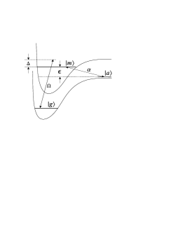
Figure 1: The energy diagrams of three-level atom-molecule system involving free-bound-bound transitions. Conversion of atoms in $\left|a\right\rangle$ to quasi-bound molecules in $\left|m\right\rangle$ is accomplished by Feshbach resonance, while the coupling between $|m\rangle$ and the ground molecular state $|g\rangle$ is provided by laser light.

One possibility to overcome the difficulty is to employ the two-photon or Raman photoassociation model, as in the proposal for generating ground molecular condensates thermal ; Mackie00 ; hope01 ; Drummond02 from atomic condensates through the stimulated Raman adiabatic passage (STIRAP) Hioe83 ; stirap . In spite of the nonlinear nature of the atom-molecule coupling in the photoassociation process, it was shown by Mackie et al. Mackie00 that in the collisionless limit, this model can support a coherent superposition of free atomic and ground molecular condensates. This superposition, being immune to the inelastic processes associated with the excited molecular state, is called the nonlinear coherent population trapping (CPT) state, in direct analogy to the CPT state in the linear $\Lambda$ three-level atomic system Alzetta76 ; Gray78 . However, efficient operation of this scheme typically demands very high laser intensities in order to overcome the weak coupling caused by the extremely small Franck-Condon overlap integral for the free atomic-bound molecular transition Drummond02 .

To overcome the small Franck-Condon factor, a Feshbach-assisted STIRAP model is proposed kokk ; mackie . Here, conversion of atoms into quasi-bound molecules is accomplished by the much more efficient Feshbach process. To bring the quasi-bound molecules into a more deeply bound vibrational state, a two-photon Raman laser field is applied. In the limit where both optical fields are tuned far-off resonance from other electronically excited levels, one can reduce the Raman coupling between the two molecular levels into an effective one-photon coupling. This leads to a three-level $\Lambda$ atom-molecule system Harris02 as shown in Fig. 1. In this scheme, the possible source of decoherence is the decay of the quasi-bound molecular state while the atomic state and the deeply bound molecular state are both stable.

In the absence of particle collisions, we expect, from the work of Mackie et al. Mackie00 , that this system is capable of supporting a CPT state, owing to the mathematical equivalence to its photoassociation counterpart. The situation when the collisions are present is more complicated. It was generally believed that the nonlinear phase shifts arising from particle collisions would defeat the two-photon resonance condition Mackie00 ; Drummond02 , a prerequisite for the existence of CPT states and hence the key for the successful implementation of STIRAP. In a recent work ling04 , we have shown that by appropriately chirping the optical frequency and the Feshbach detuning, the collision-induced nonlinear phase shifts can be dynamically compensated, hence generalizing the concept of the CPT state from the collisionless limit Mackie00 to situations where collisions cannot be ignored. In addition, we have also shown that collisions may lead to dynamical instabilities in the nonlinear CPT state, in contrast to the CPT states in the linear $\Lambda$-system which are always stable. Avoiding dynamical unstable regimes is another key for successful implementation of the STIRAP process in nonlinear systems.

The purpose of the current paper is to provide a systematic study of the excitation spectrum of the generalized nonlinear CPT state, focusing on the characterization of its stability phase diagram. To the best of our knowledge, a detailed stability analysis specific to the CPT state of the nonlinear $\Lambda$ system has never been presented before. Our paper is organized as follows: In Sec. II, we present the Hamiltonian and the nonlinear CPT solution to the coupled Gross-Pitaevskii equations. In Sec. III, collective excitations of the CPT state are calculated in the spirit of the Bogoliubov treatment bogoliubov47 ; fetter71 . Sec. IV focuses on the stability analysis in the long-wavelength limit based on the excitation spectrum obtained in Sec. III. In Sec. V, we study the dynamics of a CPT state and show that dynamical instabilities may lead to self-pulsing of a condensate mode or growth of non-condensate modes. Finally, a summary is provided in Sec. VI.

II Hamiltonian, Stationary Equations, and CPT State

We choose to formulate our theoretical description for the Feshbach-based $\Lambda$-system as illustrated in Fig. 1. The exactly same description can be applied to the two-photon photoassociation-based $\Lambda$-system, due to the formal equivalence between the two models Drummond02 . In Fig. 1, we use $|a\rangle$, $|m\rangle$, and $|g\rangle$ to denote the free atomic, quasi-bound molecular and ground molecular states, respectively. Levels $|a\rangle$ and $|m\rangle$ are coupled by a magnetic field through the Feshbach resonance with a coupling strength $\alpha$ and a detuning $\epsilon$ ($\epsilon$ is experimentally tunable via the magnetic field), while levels $|m\rangle$ and $|g\rangle$ are coupled by a (effective) laser field with a Rabi frequency $\Omega$ and a detuning $\Delta$. In second quantization, the total Hamiltonian, including collisions, takes the form

$$\hat{H} = \hbar\int d\mathbf{r}\left\{\sum_{i}\hat{\psi}_{i}^{{\dagger}}\left(\mathbf{r}\right)\left(-\frac{\hbar}{2m_{i}}\nabla^{2}\right)\hat{\psi}_{i}\left(\mathbf{r}\right)+\frac{1}{2}\sum_{i,j}\lambda_{ij}\hat{\psi}_{i}^{{\dagger}}\left(\mathbf{r}\right)\hat{\psi}_{j}^{{\dagger}}\left(\mathbf{r}\right)\hat{\psi}_{j}\left(\mathbf{r}\right)\hat{\psi}_{i}\left(\mathbf{r}\right)\right.$$ (1)

$$+\left.\epsilon\,\hat{\psi}_{m}^{{\dagger}}\left(\mathbf{r}\right)\hat{\psi}_{m}\left(\mathbf{r}\right)+\frac{\alpha}{2}\left[\hat{\psi}_{m}^{{\dagger}}\left(\mathbf{r}\right)\hat{\psi}_{a}\left(\mathbf{r}\right)\hat{\psi}_{a}\left(\mathbf{r}\right)+h.c.\right]+\left(\Delta+\epsilon\right)\hat{\psi}_{g}^{{\dagger}}\left(\mathbf{r}\right)\hat{\psi}_{g}\left(\mathbf{r}\right)-\frac{\Omega}{2}\left[\hat{\psi}_{m}^{{\dagger}}\left(\mathbf{r}\right)\hat{\psi}_{g}\left(\mathbf{r}\right)+h.c.\right]\right\},$$

where $\hat{\psi}_{i}^{{\dagger}}\left(\mathbf{r}\right)$ [$\hat{\psi}_{i}\left(\mathbf{r}\right)$] ($i=a$, $m$ and $g$) is the creation (annihilation) operator of the bosonic field for species $i$ at location $\mathbf{r}$,  and the terms proportional to $\lambda_{ij}$ represent two-body collisions with $\lambda_{ii}$ $=4\pi\hbar a_{i}/m_{i}$ and $\lambda_{ij}=\lambda_{ji}=2\pi\hbar a_{ij}/\mu_{ij}$ for $i\neq j\,$ characterizing the intra- and inter-state interaction strengths, respectively, ($a_{i}$ and $a_{ij}$ are $s$-wave scattering lengths, $m_{i}$ is the mass of species $i$ with $m_{m}=m_{g}=2m_{a}$, and $\mu_{ij}$ is the reduced mass between states $i$ and $j$). We take, without loss of generality, both $\alpha$ and $\Omega$ to be real as their phase factors can be absorbed by a trivial global gauge transformation of the field operators. Here, we consider a uniform system and hence have dropped the external trapping potentials.

Let us begin our formulation from the Bogoliubov approximation, which amounts to decomposing $\hat{\psi}_{i}\left(\mathbf{r}\right)$ as

$$\hat{\psi}_{i}\left(\mathbf{r}\right)\approx\psi_{i}\left(\mathbf{r}\right)+\delta\hat{\psi}_{i}\left(\mathbf{r}\right),$$ (2)

where $\psi_{i}\left(\mathbf{r}\right)=\left\langle\hat{\psi}_{i}\left(\mathbf{r}\right)\right\rangle$ is the condensate wave function and $\delta\hat{\psi}_{i}\left(\mathbf{r}\right)$ is a small fluctuation field operator that obeys the usual bosonic commutation relation

$$\left[\delta\hat{\psi}_{i}\left(\mathbf{r}\right),\delta\hat{\psi}_{j}^{{\dagger}}\left(\mathbf{r}^{\prime}\right)\right]=\delta_{ij}\delta\left(\mathbf{r-r}^{\prime}\right).$$ (3)

As a first step in the Bogoliubov approach, we put Eq. (2) into the grand canonical Hamiltonian (1)

$$\mathcal{\hat{H}}=\hat{H}-\hbar\mu\int d\mathbf{r}\left[\hat{\psi}_{a}^{{\dagger}}\hat{\psi}_{a}+2\hat{\psi}_{m}^{{\dagger}}\hat{\psi}_{m}+2\hat{\psi}_{g}^{{\dagger}}\hat{\psi}_{g}\right],$$ (4)

where the chemical potential $\hbar\mu$ is introduced to conserve the total particle number, and expand Eq. (4) up to the second order in fluctuation operators as

$$\mathcal{\hat{H}}\approx\mathcal{\hat{H}}^{\left(0\right)}+\mathcal{\hat{H}}^{\left(1\right)}+\mathcal{\hat{H}}^{\left(2\right)},$$ (5)

where the subscript represents the order in $\delta\hat{\psi}_{i}\left(\mathbf{r}\right)$.

The zeroth order term, $\mathcal{\hat{H}}^{\left(0\right)}$, is a constant depending on the wave functions $\psi_{i}$ and is irrelevant to our interest. The first-order term, $\mathcal{\hat{H}}^{\left(1\right)}$, is required to vanish in the Bogoliubov formalism. This requirement leads to a set of coupled stationary equations

$$\mu\psi_{a} = \left(-\frac{\hbar\nabla^{2}}{2m_{a}}+\sum_{i}\lambda_{ai}\left|\psi_{i}\right|^{2}\right)\psi_{a}+\alpha\psi_{m}\psi_{a}^{\ast},$$ (6a)

$$2\mu\psi_{m} = \left(-\frac{\hbar\nabla^{2}}{4m_{a}}+\sum_{i}\lambda_{mi}\left|\psi_{i}\right|^{2}\right)\psi_{m}+\epsilon\psi_{m}+\frac{\alpha}{2}\psi_{a}^{2}$$ (6b)

$$\;\;\;\;\;\;-\frac{\Omega}{2}\psi_{g},$$

$$2\mu\psi_{g} = \left(-\frac{\hbar\nabla^{2}}{4m_{a}}+\sum_{i}\lambda_{gi}\left|\psi_{i}\right|^{2}\right)\psi_{g}+\left(\Delta+\epsilon\right)\psi_{g}$$ (6c)

$$\;\;\;\;\;\;-\frac{\Omega}{2}\psi_{m},$$

which represent the generalized time-independent Gross-Pitaevskii equations (GPEs). Finally, the second-order term, $$\mathcal{\hat{H}}^{\left(2\right)}$$, which has a more complicated structure, will be studied separately in the next section where we calculate the spectra of the collective excitations.

We now turn our attention to the homogeneous (zero-momentum) solution to the GPEs. To proceed, we separate each wave function into an amplitude and a phase according to

$$\psi_{j}=\left|\psi_{j}\right|e^{i\theta_{j}},\;\;j=a,m,g.$$ (7)

To seek the CPT solution, we take $\psi_{m}=0$. After substituting Eq. (7) into Eq. (6), we find that under the conditions

$$\theta_{g} = 2\theta_{a},$$

$$\alpha\left|\psi_{a}\right|^{2} = \Omega\left|\psi_{g}\right|,$$ (8)

Eq. (6) possesses a solution consistent with the requirement that $\psi_{m}=0$. The explicit form of this solution can be readily found by combining Eq. (8 ) with the particle number conservation

$$\left|\psi_{a}\right|^{2}+2\left|\psi_{g}\right|^{2}=n,$$ (9)

where $n$ is the total particle density, to yield the particle density distribution as

$$\left|\psi_{m}^{0}\right|^{2} = 0\,,$$ (10a)

$$\left|\psi_{a}^{0}\right|^{2} = \frac{2n}{1+\sqrt{1+8\left(\frac{\alpha\sqrt{n}}{\Omega}\right)^{2}}}\,,$$ (10b)

$$\left|\psi_{g}^{0}\right|^{2} = \frac{n}{2}\frac{\sqrt{1+8\left(\frac{\alpha\sqrt{n}}{\Omega}\right)^{2}}-1}{1+\sqrt{1+8\left(\frac{\alpha\sqrt{n}}{\Omega}\right)^{2}}}\,.$$ (10c)

A check for consistency leads to the chemical potential

$$\mu=\lambda_{a}\left|\psi_{a}^{0}\right|^{2}+\lambda_{ag}\left|\psi_{g}^{0}\right|^{2},$$ (11)

where $\lambda_{i}\equiv\lambda_{ii}$, and the laser detuning

$$\Delta=-\epsilon+\left(2\lambda_{ag}-\lambda_{g}\right)\left|\psi_{g}^{0}\right|^{2}+\left(2\lambda_{a}-\lambda_{ag}\right)\left|\psi_{a}^{0}\right|^{2},$$ (12)

which is necessary in order for Eqs. (10) to be a stationary solution of Eqs. (6).

The vanishing of the population in the quasi-bound molecular state indicates a destructive interference in the excitation to this state. A system prepared in the state represented by Eqs. (10) is not subject to the particle loss suffered by the quasi-bound molecular state. This situation is reminiscent of the CPT state in a linear $\Lambda$-type atomic system where the atoms are immune to the spontaneous emission Alzetta76 ; Gray78 . For this reason, we regard the steady state represented by Eqs. (10) as the nonlinear matter-wave analog of the CPT state in a linear $\Lambda$-system.

Interestingly, just as in the linear case, the CPT solution described by Eqs. (10) depends only explicitly on the two coupling strengths, $\alpha$ and $\Omega$, not on the collisional parameters. The latter, however, play important roles as evidenced by Eq. (12). Note that in the absence of collisions, Eq. (12) degenerates into $\Delta+\epsilon=0$, which is just the ordinary “two-photon” resonance condition. Thus, Eq. (12) can be regarded as the generalization of the two-photon resonance in which the nonlinear phase shifts due to particle collisions have been compensated. This CPT solution is therefore a nonlinear generalization of the one found in the collisionless limit Mackie00 .

III Collective Excitations of the CPT State

In this section, we want to calculate the excitation spectra of the CPT state, especially, the spectra in the long-wavelength limit, since they determine many important properties, including the stability, of the CPT state at low temperature.

III.1 Bogoliubov Equations

To determine the equations for the collective excitations, we first take advantage of our system being homogeneous and move to the momentum space through the expansion

$$\delta\hat{\psi}_{i}\left(\mathbf{r}\right)=\frac{1}{\left(2\pi\hbar\right)^{3/2}}\int d\mathbf{p}\,e^{i\mathbf{p\cdot r/\hbar}}\,\hat{c}_{i}\left(\mathbf{p}\right)\,,$$ (13)

where $\hat{c}_{i}\left(\mathbf{p}\right)$ [$\hat{c}_{i}^{{\dagger}}\left(\mathbf{p}\right)$] is the annihilation (creation) operator for a particle of species $i$ with momentum $\mathbf{p}$ and obey the standard bosonic commutation relation

$$\left[\hat{c}_{i}\left(\mathbf{p}\right),\hat{c}_{j}^{{\dagger}}\left(\mathbf{p}^{\prime}\right)\right]=\delta_{ij}\delta\left(\mathbf{p-p}^{\prime}\right),$$ (14)

in accordance with Eq. (3). The third term $\mathcal{\hat{H}}^{\left(2\right)}$ in Eq. (5) for our CPT state can now be put into a compact form

$$\mathcal{\hat{H}}^{\left(2\right)} = \frac{\hbar}{2}\int d\mathbf{p}^{\prime}\sum_{nm}\left\{2\hat{c}_{n}^{{\dagger}}\left(\mathbf{p}^{\prime}\right)\left(A\right)_{nm}\hat{c}_{m}\left(\mathbf{p}^{\prime}\right)\right.$$ (15)

$$+\left.\left[\hat{c}_{n}\left(\mathbf{p}^{\prime}\right)B_{nm}\hat{c}_{m}\left(-\mathbf{p}^{\prime}\right)+h.c.\right]\right\},$$

where $A$ and $B$ are both real and symmetric matrices, given by

$$A = \left(\begin{array}[]{ccc}\epsilon_{p}+\lambda_{a}\left|\psi_{a}^{0}\right|^{2}&\alpha\left|\psi_{a}^{0}\right|&\lambda_{ag}\left|\psi_{a}^{0}\right|\left|\psi_{g}^{0}\right|\\ \alpha\left|\psi_{a}^{0}\right|&\frac{\epsilon_{p}}{2}+\epsilon^{\prime}&-\frac{\Omega}{2}\\ \lambda_{ag}\left|\psi_{a}^{0}\right|\left|\psi_{g}^{0}\right|&-\frac{\Omega}{2}&\frac{\epsilon_{p}}{2}+\lambda_{g}\left|\psi_{g}^{0}\right|^{2}\end{array}\right),$$ (16d)

$$B = \left(\begin{array}[]{ccc}\lambda_{a}\left|\psi_{a}^{0}\right|^{2}&0&\lambda_{ag}\left|\psi_{a}^{0}\right|\left|\psi_{g}^{0}\right|\\ 0&0&0\\ \lambda_{ag}\left|\psi_{a}^{0}\right|\left|\psi_{g}^{0}\right|&0&\lambda_{g}\left|\psi_{g}^{0}\right|^{2}\end{array}\right),$$ (16h)

where we have defined

$$\epsilon_{p} \equiv p^{2}/(2m_{a}\hbar)\,,$$ (17a)

$$\epsilon^{\prime} = \epsilon-\Lambda_{a}\left|\psi_{a}^{0}\right|^{2}-\Lambda_{g}\left|\psi_{g}^{0}\right|^{2}\,,$$ (17b)

$$\Lambda_{a} = 2\lambda_{a}-\lambda_{am}\,,$$ (17c)

$$\Lambda_{g} = 2\lambda_{ag}-\lambda_{mg}\,.$$ (17d)

The process of finding the quasiparticle spectrum begins by changing Eq. (15) into a diagonalized form

$$\mathcal{\hat{H}}^{\left(2\right)}=\hbar\int d\mathbf{p}\sum_{i}\omega_{i}\left(p\right)\hat{b}_{i}^{{\dagger}}\left(\mathbf{p}\right)\hat{b}_{i}\left(\mathbf{p}\right)+c{\rm-number},$$ (18)

with the generalized Bogoliubov transformation

$$\hat{b}_{i}\left(\mathbf{p}\right)=\sum_{j}u_{ij}\left(p\right)\hat{c}_{j}\left(\mathbf{p}\right)+\sum_{j}v_{ij}\left(p\right)\hat{c}_{j}^{{\dagger}}\left(-\mathbf{p}\right),$$ (19)

where $\omega_{i}\left(p\right)$ is the quasiparticle frequency, $u_{ij}\left(p\right)$ and $v_{ij}\left(p\right)$ are the transformation coefficients, and $\hat{b}_{i}\left(\mathbf{p}\right)$ and $\hat{b}_{i}^{{\dagger}}\left(\mathbf{p}\right)$ are the respective annihilation and creation operators for a quasiparticle of frequency $\omega_{i}\left(p\right)$ and momentum $\mathbf{p}$. To obtain the equations for $\omega_{i}\left(p\right)$, $u_{ij}\left(p\right)$ and $v_{ij}\left(p\right)$, we first note that

$$\left[\hat{b}_{i}\left(\mathbf{p}\right),\mathcal{\hat{H}}^{\left(2\right)}\right]=\hbar\omega_{i}\left(p\right)\hat{b}_{i}\left(\mathbf{p}\right).$$ (20)

Inserting Eq. (19) into Eq. (20) and with the help of Eqs. (14) and (15) along with the symmetric properties of $A$ and $B$, we arrive at

$$\sum_{m}\sum_{n}\left\{\left[A_{mn}u_{in}-B_{mn}v_{in}\right]\hat{c}_{m}\left(\mathbf{p}\right)+\left[B_{mn}u_{in}-A_{mn}v_{in}\right]\hat{c}_{m}^{{\dagger}}\left(-\mathbf{p}\right)\right\}=\omega_{i}\sum_{m}\left[u_{im}\hat{c}_{m}\left(\mathbf{p}\right)+v_{im}\hat{c}_{m}^{{\dagger}}\left(-\mathbf{p}\right)\right].$$ (21)

Equating the coefficients of $\hat{c}_{m}\left(\mathbf{p}\right)$ and $\hat{c}_{m}^{{\dagger}}\left(-\mathbf{p}\right)$ on both sides of the above equation, we arrive at a 6$\times 6$ matrix equation

$$\left(\begin{array}[]{cc}A&-B\\ B&-A\end{array}\right)\left(\begin{array}[]{c}u_{i}\\ v_{i}\end{array}\right)=\omega_{i}\left(p\right)\left(\begin{array}[]{c}u_{i}\\ v_{i}\end{array}\right),$$ (22)

where

$$u_{i}=\left(u_{ia},u_{im},u_{ig}\right)^{T},\;\;\;v_{i}=\left(v_{ia},v_{im},v_{ig}\right)^{T}.$$

A simple manipulation can show that $\omega_{i}^{2}(p)$ are the eigenvalues of the $3\times 3$ matrix $(A+B)(A-B)$, hence $\omega_{i}^{2}(p)$ satisfy a cubic equation with the form

$$\left(\omega_{i}^{2}\right)^{3}-a_{1}\left(\omega_{i}^{2}\right)^{2}+a_{2}\omega_{i}^{2}-a_{3}=0\,,$$ (23)

where the coefficients are given by

$$a_{1} = a_{10}+a_{11}\epsilon_{p}+a_{12}\epsilon_{p}^{2}\,,$$ (24a)

$$a_{2} = a_{20}+a_{21}\epsilon_{p}+a_{22}\epsilon_{p}^{2}+a_{23}\epsilon_{p}^{3}+a_{24}\epsilon_{p}^{4}\,,$$ (24b)

$$a_{3} = a_{31}\epsilon_{p}+a_{32}\epsilon_{p}^{2}+a_{33}\epsilon_{p}^{3}+a_{34}\epsilon_{p}^{4}+$$ (24c)

$$a_{35}\epsilon_{p}^{5}+a_{36}\epsilon_{p}^{6}\,.$$

The coefficients $a_{ij}$ depend on the coupling and the collisional constants and are in general quite complicated. We only list three of them below

$$a_{10} = \epsilon^{\prime 2}+\frac{1}{2}\left(\Omega^{2}+4\alpha^{2}\left|\psi_{a}^{0}\right|^{2}\right)\,,$$ (25a)

$$a_{20} = \frac{1}{16}\left(\Omega^{2}+4\alpha^{2}\left|\psi_{a}^{0}\right|^{2}\right)^{2}-0.5\epsilon^{\prime}\alpha^{2}\left|\psi_{a}^{0}\right|^{4}\left(\lambda_{g}-4\lambda_{ag}+4\lambda_{a}\right)\,,$$ (25b)

$$a_{31} = \frac{1}{8}\left|\psi_{a}^{0}\right|^{2}\left(\Omega^{2}+2\alpha^{2}\left|\psi_{a}^{0}\right|^{2}\right)\times\left[\lambda_{a}\Omega^{2}+4\alpha^{2}\left(\lambda_{g}\left|\psi_{g}^{0}\right|^{2}+\lambda_{ag}\left|\psi_{a}^{0}\right|^{2}\right)-8\epsilon^{\prime}\left(\lambda_{a}\lambda_{g}-\lambda_{ag}^{2}\right)\left|\psi_{g}^{0}\right|^{2}\right]\,,$$ (25c)

as they will be explicitly referenced in later discussions.

III.2 Excitation Spectra

Equation (23) has a cubic form with respect to $\omega_{i}^{2}$ and hence can be solved analytically. However the analytical expressions are in general too complicated to provide much physical insights. Since we are most interested in the long-wavelength excitations, we proceed to take a perturbative approach by expanding $\omega_{i}(p)$ in the limit of small $p$, or equivalently, small $\sqrt{\epsilon_{p}}$. The perturbative solution thus takes the form:

$$\omega_{i}\left(p\right)\approx\omega_{i}^{\left(0\right)}+d_{i}^{\left(1\right)}\,\sqrt{\epsilon_{p}}+d_{i}^{\left(2\right)}\,\epsilon_{p}+\cdots,$$ (26)

In order to bring out the effects of collisions more clearly, let us first consider the collicionless limit.

III.2.1 Excitation Spectra in the Collisionless Limit

In the absence of collisions, the matrix $B$ becomes null. The excitation frequencies $\omega_{i}(p)$ are eigenvalues of the Hermitian matrix $A$ and therefore must be real. This means that there is no dynamical instability in spite of the nonlinear nature of the coupling between the atomic and the quasi-bound molecular state.

To the zeroth order, we find that $\omega_{i}^{\left(0\right)}$ has three solutions comment

$$\omega_{0}^{\left(0\right)}=0,\;\;\;\omega_{\pm}^{\left(0\right)}=\sqrt{\left(a_{10}\pm\sqrt{a_{10}^{2}-4a_{20}}\right)/2}\,,$$ (27)

where the subscripts $\left(0,-,+\right)$ are used to denote the three branches of the collective modes. Clearly the 0-branch is gapless, while the $(\pm)$-branches are gapped. The reality of $\omega_{\pm}^{\left(0\right)}$ is guaranteed because here both $a_{10}$ and $a_{20}$ are positive with $a_{10}^{2}\geq 4a_{20}$ [see Eqs. (25a) and (25b), in the absence of collisions.]

For all three branches, we have found that $d_{i}^{(1)}=0$. Hence the next leading order in $\omega_{i}(p)$ is quadratic in momentum with

$$d_{0}^{(2)} = \frac{\Omega^{2}+2\alpha^{2}\left|\psi_{a}^{0}\right|^{2}}{\Omega^{2}+4\alpha^{2}\left|\psi_{a}^{0}\right|^{2}}\,,$$ (28a)

$$d_{\pm}^{\left(2\right)} = \pm\frac{\left[\frac{\Omega^{2}}{8}+\alpha^{2}\left|\psi_{a}^{0}\right|^{2}+\frac{(\omega_{\pm}^{(0)})^{2}}{2}\right]}{\left[(\omega_{\pm}^{(0)})^{2}+\frac{\Omega^{2}}{4}+\alpha^{2}\left|\psi_{a}^{0}\right|^{2}\right]}\,,$$ (28b)

Figure 2: The quasiparticle dispersion spectra for $n=1$, $\Omega=$ $1$, and $\epsilon=-2$. Solid lines represent the collisionless case while dotted lines are for a system with $\lambda_{a}=0.625,$ $\lambda_{m}=\lambda_{g}=\lambda_{am}=\lambda_{ag}=\lambda_{mg}=0.3\lambda_{a}$. Units are defined in Sec. IV.

Solid lines in Fig. 2 represent the three branches in the collisionless limit. They are obtained by directly solving the cubic equation (23), and are in good agreement with the perturbative results (not shown).

III.2.2 Excitation Spectra with Collisions

The spectra including the collisional terms can be similarly obtained. The zeroth order solutions, $\omega_{i}^{(0)}$, have exactly the same forms as in the collisionless limit given by Eq. (27). Therefore the 0-branch continues to be gapless. Due to the collision-modified coefficients $a_{ij}$, the two zeroth order gapped modes $\omega_{\pm}^{(0)}$ are now, however, no longer guaranteed to be real. Complex mode frequencies lead to the dynamical instability, which we will discuss in detail in the next section.

Another important effect of the collisions is the modification of the gapless 0-branch. While $d_{\pm}^{(1)}$ still remains to be zero (hence the two gapped branches are still quadratic in $p$ to the leading order), $d_{0}^{(1)}$ now takes a finite value given by

$$d_{0}^{\left(1\right)}=\sqrt{\frac{a_{31}}{a_{20}}},$$ (29)

Hence the gapless branch, in the long-wavelength limit, is linear in $p$ and represents the phonon mode with the speed of sound determined by Eq. (29). The dotted lines in Fig. 2 represent the spectra with collisions in the stable regime. Once again, they are calculated by solving the cubic Eq. (23), but are found in good agreement with the perturbative results (not shown).

According to Eq. (29), whenever $a_{31}$ and $a_{20}$ are opposite in sign, $\omega_{0}$ becomes imaginary for finite $p$ in the long wavelength limit, indicating an unstable 0-branch. We now turn to a detailed discussion of the collision-induced dynamical instability. Note that from Eq. (29), it may seem that $\omega_{0}$ is singular for any finite momenta when $a_{20}=0$. However, when $a_{20}=0,\omega_{0}^{\left(0\right)}$ and $\omega_{-}^{\left(0\right)}$ are degenerate according to Eq. (27). Thus, this singularity is only an artefact, indicating the failure of the nondegenerate perturbative calculation. Indeed, exact solutions of Eq. (23) do not exhibit such a singularity. Despite of this complication, the perturbative results can be used to identify the unstable regimes quite accurately.

IV Classification of Dynamical Instability

Studies in Sec. III.2.2 suggest that complex excitation frequencies and hence dynamical instabilities can occur under the following situations:

1. When $a_{31}$ and $a_{20}$ possess opposite signs, 0-branch becomes unstable [see Eq. (29)];

2. When $a_{20}<0$, $\omega_{-}$ becomes complex [see Eq. (27)];

3. When $a_{10}^{2}<4a_{20}$, both $(\pm)$-branches become unstable [see Eq. (27)].

Before moving foward, let us clarify our unit system. We consider systems with particle densities in the order of $n_{0}=5\times 10^{20}$ m^-3, and $\alpha$ fixed to $4.22\times 10^{-6}$ m^3/2s^-1, which corresponds to the atom-molecule coupling strength for the ²³Na Feshbach resonance at a magnetic field strength of $85.3$ mT seaman03 . We then adopt a unit system in which $n_{0}$ is the unit for density, $\alpha/\sqrt{n_{0}}=1.88724\times 10^{-16}$m³s^-1 the unit for collisional parameters ($\lambda_{i}$, $\lambda_{ij}$), $\alpha\sqrt{n_{0}}=9.436\times 10^{4}$ s^-1 the unit for frequencies $\left(\omega,\Omega,\epsilon\right)$, and $\sqrt{\left(2m\hbar\alpha\sqrt{n_{0}}\right)}=8.72\times 10^{-28}$ kg m/s the unit for momentum $p$. Furthermore, for simplicity, we only consider the situation where all the scattering lengths are positive.

Our goal is to identify the unstable regimes in the parameter space spanned by $\epsilon$ and $\Omega$, while the laser detuning $\Delta$ is always fixed by the resonance condition represented by Eq. (12). For cases 1 and 2, we can identify two threshold values for the Feshbach detuning $\epsilon_{0}^{th}$ and $\epsilon_{1}^{th}$, given by

$$\epsilon_{0}^{th} = \Lambda_{a}\left|\psi_{a}^{0}\right|^{2}+\Lambda_{g}\left|\psi_{g}^{0}\right|^{2}+\frac{2\left(\frac{\Omega^{2}}{4|\psi_{a}^{0}|^{2}}+1\right)^{2}}{4\lambda_{a}+\lambda_{g}-4\lambda_{ag}},$$ (30)

$$\epsilon_{1}^{th} = \Lambda_{a}\left|\psi_{a}^{0}\right|^{2}+\Lambda_{g}\left|\psi_{g}^{0}\right|^{2}$$ (31)

$$\;+\frac{\lambda_{a}\Omega^{2}+4\left(\lambda_{g}\left|\psi_{g}^{0}\right|^{2}+\lambda_{ag}\left|\psi_{a}^{0}\right|^{2}\right)}{8\left|\psi_{g}^{0}\right|^{2}\left(\lambda_{a}\lambda_{g}-\lambda_{ag}^{2}\right)},$$

which are obtained from the conditions $a_{20}=0$ and $a_{31}=0$, respectively. Case 3 will be discussed at the end of this section.

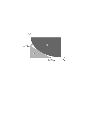
Figure 3: Division of the positive quarter of $\left(\lambda_{g},\lambda_{a}\right)$-space into three regions by a straight line: $\lambda_{g}=-4\lambda_{a}+4\lambda_{ag}$ and a hyperbola: $\lambda_{a}\lambda_{g}=\lambda_{ag}^{2}$.

It is not difficult to see that the signs of the denominators of the last terms of (30) and (31), $4\lambda_{a}+\lambda_{g}-4\lambda_{ag}$ and $\lambda_{a}\lambda_{g}-\lambda_{ag}^{2}$, respectively, will play crucial roles in locating the instability parameter regime. For this reason, we first decompose the $\left(\lambda_{g}\text{,}\lambda_{a}\right)$-space into three regions divided by a straight line, $\lambda_{g}=-4\lambda_{a}+4\lambda_{ag}$, and a hyperbola, $\lambda_{a}\lambda_{g}=\lambda_{ag}^{2}$, as shown in Fig. 3. The line is tangent to the hyperbola at the point $\left(\lambda_{g}=2\lambda_{ag}\text{,}\lambda_{a}=0.5\lambda_{ag}\right)$. The three regions are defined as follows: Both $4\lambda_{a}+\lambda_{g}-4\lambda_{ag}$ and $\lambda_{a}\lambda_{g}-\lambda_{ag}^{2}$ are negative in Region I and both are positive in Region II, while in Region III, $4\lambda_{a}+\lambda_{g}-4\lambda_{ag}<0$ and $\lambda_{a}\lambda_{g}-\lambda_{ag}^{2}>0$.

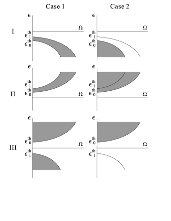
Figure 4: Classification of the instabilities in the limit of low momentum. The shaded areas of the diagrams in column one and two correspond to the instabilities due to the imaginary sound speed and the complex gaps, respectively. Each set of diagrams in row 1, 2 and 3 are the instability maps for systems operating in region I, II, and III as specified in Fig. 3, respectively.

Next, we choose to construct, for each region defined above, two instability maps in the $\left(\Omega,\epsilon\right)$-space; one for the instability due to the imaginary sound speed (case 1), and the other for the instability due to the complex gap (case 2). We represent them by the shaded areas of the diagrams in the first and second columns of Fig. 4, respectively. Each set of diagrams in row 1, 2 and 3 are built upon the collisional parameters corresponding to Regions I, II, and III of $\left(\lambda_{g}\text{,}\lambda_{a}\right)$-space, respectively. We construct these maps based on two principles. First, it can be shown from Eqs. (30) and (31) that $\epsilon_{1}^{th}-\epsilon_{0}^{th}\propto 1/\left(4\lambda_{a}+\lambda_{g}-4\lambda_{ag}\right)\left(\lambda_{a}\lambda_{g}-\lambda_{ag}^{2}\right)$ with a positive definite proportionality.  As a result, we have $\epsilon_{1}^{th}>\epsilon_{0}^{th}$ in Regions I and II, and $\epsilon_{1}^{th}<\epsilon_{0}^{th}$ in Region III. Second, according to Eq. (39) [Eq. (40 )], $\epsilon_{0}^{th}$ [$\epsilon_{1}^{th}$] is bent downward if $4\lambda_{a}+\lambda_{g}-4\lambda_{ag}$  $<0$ [$\lambda_{a}\lambda_{g}-\lambda_{ag}^{2}$ $<0$] and vice versa. Note that the instability of case 2 is solely determined by $\epsilon_{0}^{th}$; the presence of $\epsilon_{1}^{th}$ in the second column of Fig. 4 is to make the comparison of the two maps easier. For example, one can easily identify that the two instability maps in region II overlap in the band between $\epsilon_{0}^{th}$ and $\epsilon_{1}^{th}$.

Let us now consider a specific atom-molecule system composed of ²³Na. The atomic $s$-wave scattering length for sodium is around $a_{a}=3.4$ nm abeelen99 which yields $\lambda_{a}=0.625$. No precise knowledge about the scattering lengths involving molecules exists. Assuming they are on the same order of magnitude as $a_{a}$, we take $\lambda_{m}=\lambda_{g}=\lambda_{am}=\lambda_{mg}=\lambda_{ag}=0.3\lambda_{a}$. This set of parameters puts the system in Region II of Fig. 4. According to Eqs. (41) and (42), $\epsilon_{0}^{th}$ and $\epsilon_{1}^{th}$ approach $0.5\Lambda_{g}+2\alpha^{2}/\left(4\lambda_{a}+\lambda_{g}-4\lambda_{ag}\right)=1.126$ and $0.5\Lambda_{g}+0.5\alpha^{2}\lambda_{g}/\left(\lambda_{a}\lambda_{g}-\lambda_{ag}^{2}\right)=1.237,$ respectively, in the limit of small $\Omega$.

Figure 5: Im$\left[\omega\left(p\right)\right]$ as a function of $\Omega$ for a fixed momentum $p=0.005$. The curves from left to right correspond to $\epsilon=1.3$, $\epsilon=1.5$, $\epsilon=2,$ and $\epsilon=3$, respectively. Other parameters are $n=1$, $\lambda_{a}=0.625,$ and $\lambda_{m}=\lambda_{g}=\lambda_{am}=\lambda_{mg}=\lambda_{ag}=0.3\lambda_{a}$. Units are defined in Sec. IV.

A search using Eq. (23) above these thresholds and at small momenta indeed leads to two branches whose frequencies have finite imaginary parts for certain values of $\Omega$, as illustrated in Fig. 5(a) and (b), respectively. Each curve in Fig. 5(a) is restricted between two thresholds, both of which increase as $\epsilon$, evidently resembling the instability originating from the imaginary sound speed (case 1). Thus, in the limit of small $p$, we expect it to approach $d_{0}^{\left(1\right)}p$. In fact, one can trace the sharp asymmetry of each curve to the fact that according to Eq. (29), $d_{0}^{\left(1\right)}$ vanishes at the left threshold where $a_{31}$ is close to zero, while becomes singular at the right threshold where $a_{20}$ is close to zero. In contrast, each curve in Fig. 5(b) has only one threshold, which matches quite closely to the right threshold of the corresponding curve in Fig. 5(a). This along with the fact that the value of the mode frequency is rather insensitive with respect to $p$ (as long as $p$ is not too large) indicates that it represents the instability from the complex gapped branch of case 2. Therefore these exact calculations are in good agreement with the insights gained from the instability map shown in Fig. 4.

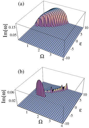
Figure 6: (Color online) A three-dimensional view of Im$\left[\omega\left(p\right)\right]$ as a function of $\Omega$ and $\epsilon$ for two branches of roots to Eq.(23). Parameters are same as in Fig. 5. Units are defined in Sec. IV.

In order to have a more detailed look at various instabilities, we make a three-dimensional plot in Fig. 6 for the imaginary parts of the two (non-vanishing) branches of excitation frequencies. A glance at this 3D view further confirms the instability map of Fig. 4: one can easily associate the large bump in Fig. 6(a) to the instability of case 2, and the curved band in Fig. 6(b) to the instability of case 1. The shapes of these unstable regions completely match with those shown in Fig. 4.

However, Fig. 6(b) also reveals a new feature consisting of a narrow strip along the $\Omega$ dimension. We can trace this new feature to the source of instability associated with case 3 which has so far been ignored. An analysis with the help of Eqs. (25a) and (25b) indicates that the condition $a_{20}>a_{10}^{2}/4$ amounts to

$$\epsilon^{\prime}\left[\epsilon^{\prime 3}+\left(\Omega^{2}+4\alpha^{2}\left|\psi_{a}^{0}\right|^{2}\right)\epsilon^{\prime}\right.$$

$$\left.+2\alpha^{2}\left|\psi_{a}^{0}\right|^{4}\left(\lambda_{g}-4\lambda_{ag}+4\lambda_{a}\right)\right]<0,$$ (32)

from which we find that to a good approximation, the unstable $\epsilon$ is bounded between

$$\epsilon_{1} = \Lambda_{a}\left|\psi_{a}^{0}\right|^{2}+\Lambda_{g}\left|\psi_{g}^{0}\right|^{2}\,,$$ (33a)

$$\epsilon_{2} \approx \epsilon_{1}-2\alpha^{2}\left|\psi_{a}^{0}\right|^{4}\,\frac{\lambda_{g}-4\lambda_{ag}+4\lambda_{a}}{\Omega^{2}+4\alpha^{2}\left|\psi_{a}^{0}\right|^{2}}\,,$$ (33b)

It can be shown that $\epsilon_{1}$ and $\epsilon_{2}$ are not very sensitive to $\Omega$, and the they merge together in the limit of either small or large $\Omega$, which explains the shape of this new instability region.

V Dynamical Signatures of Stable and Unstable CPT states

In order to determine the fate of an unstable state, we must examine its dynamical response to fluctuations, which can be simulated using the time-dependent version of the GPEs, which are obtained by replacing the left hand sides of Eqs. (6) by $i\dot{\psi}_{i}$.

We take a CPT state associated with a Rabi frequency $\Omega_{0}$ and Feshbach detuning $\epsilon$ to be the initial state. To simulate small fluctuations, we modify the Rabi frequency as

$$\Omega=\Omega_{0}+\left[\delta\Omega_{0}+2\delta\Omega_{1}\sin\left(px/\hbar\right)\right],$$ (34)

where $\delta\Omega_{0}$ and $\delta\Omega_{1}$ are small perturbation amplitudes. Note that a position-dependent perturbation represented by the $\delta\Omega_{1}$ term can cause spatial deformation of the uniform CPT state, making it possible to trigger the instabilities due to perturbations of finite momentum.

Figure 7: The time evolution of the particle number densities in the condensate mode probed by a zero-momentum perturbation with $\delta\Omega_{0}=0.001$ for (a) $\Omega_{0}=1.1$ and (b) $\Omega=0.9$, while the Feshbach detuning is fixed at $\epsilon=3$. Other parameters are the same as in Fig. 5. Units are defined in Sec. IV.

To test the instability of case 2, we take the same collisional parameters as in Fig. 5, but fix the Feshbach detuning to $\epsilon=3$. We apply a zero-momentum perturbation with an amplitude $\delta\Omega_{0}=0.001$ and $\delta\Omega_{1}=0$ to the CPT state with (a) $\Omega_{0}=1.1$ and (b) $\Omega_{0}=0.9$, respectively. By inspecting the $\epsilon=3$ curve of Fig. 5(b), which survives even when $p=0$, we anticipate that the dynamics of the system will change from a stable to an unstable one as $\Omega_{0}$ varies from $1.1$ to $0.9$. The results, shown in Fig. 7(a) and (b), clearly support our analysis. The stable CPT state does not respond significantly to the small perturbation; while Fig. 7(b) shows a large-amplitude self-pulsing behavior, characteristic of an unstable system. In addition, there is a noticeable population in the unstable molecular state. Such self-pulsing oscillations are also familiar features in the study of unstable nonlinear optical systems pierre .

To demonstrate the instability of case 1, we need to apply a finite-momentum perturbation since for case 1, the imaginary part of the excitation frequency $\omega_{0}$ vanishes at $p=0$. The finite-momentum perturbation will couple together different momentum modes. To simulate this process, we adopt the Floquet technique and expand the wave functions as

$$\psi_{i}\left(\mathbf{r},t\right)=\sum_{l=-\infty}^{+\infty}\phi_{i}\left(l,t\right)e^{ilpx/\hbar}\,,$$ (35)

where $\left|\phi_{i}\left(l,t\right)\right|^{2}$ represent the particle density of the $i$th species with momentum $lp$.  Here, $l$ is an integer and $p=2\pi\hbar/L$, with $L$ being the length of the condensate along $x$ dimension. Then the orthonormality condition for the momentum modes reads

$$\frac{1}{L}\,\int e^{i\left(l-l^{\prime}\right)px/\hbar}dx=\delta_{l,l^{\prime}}\,.$$ (36)

This enables us to transform the dynamical GPEs for $\psi_{i}\left(\mathbf{r},t\right)$ into the coupled modal equations for $\phi_{i}\left(l,t\right)$

$$i\frac{d\phi_{a}\left(n\right)}{dt} = -\epsilon_{p}n^{2}\phi_{a}\left(n\right)+\sum_{l,l^{\prime}}\sum_{s}\lambda_{as}\phi_{s}\left(l\right)\phi_{s}^{\ast}\left(l^{\prime}\right)\phi_{a}\left(n+l^{\prime}-l\right)+\alpha\sum_{l}\phi_{m}\left(l\right)\phi_{a}^{\ast}\left(l-n\right)\,,$$ (37a)

$$i\frac{d\phi_{m}\left(n\right)}{dt} = -\frac{\epsilon_{p}}{2}n^{2}\phi_{m}\left(n\right)+\sum_{l,l^{\prime}}\sum_{s}\lambda_{ms}\phi_{s}\left(l\right)\phi_{s}^{\ast}\left(l^{\prime}\right)\phi_{m}\left(n+l^{\prime}-l\right)+\epsilon\phi_{m}\left(n\right)$$ (37b)

$$+\frac{\alpha}{2}\sum_{l}\phi_{a}\left(l\right)\phi_{a}\left(n-l\right)-\frac{\Omega_{0}+\delta\Omega_{0}}{2}\phi_{g}\left(n\right)-\frac{\delta\Omega_{1}}{2i}\left[\phi_{g}\left(n-1\right)-\phi_{g}\left(n+1\right)\right]\,,$$

$$i\frac{d\phi_{g}\left(n\right)}{dt} = -\frac{\epsilon_{p}}{2}n^{2}\phi_{g}\left(n\right)+\sum_{l,l^{\prime}}\sum_{s}\lambda_{gs}\phi_{s}\left(l\right)\phi_{s}^{\ast}\left(l^{\prime}\right)\phi_{g}\left(n+l^{\prime}-l\right)+\left(\Delta+\epsilon\right)\phi_{g}\left(n\right)$$ (37c)

$$-\frac{\Omega_{0}+\delta\Omega_{0}}{2}\phi_{m}\left(n\right)-\frac{\delta\Omega_{1}}{2i}\left[\phi_{m}\left(n-1\right)-\phi_{m}\left(n+1\right)\right]\,.$$

The initial condition is then equivalent to

$$\phi_{a}\left(0,0\right)=\left|\psi_{a}^{0}\right|,\phi_{m}\left(0,0\right)=0,\phi_{g}\left(0,0\right)=\left|\psi_{g}^{0}\right|\,,$$ (38)

and $\phi_{i}\left(l\neq 0,0\right)=0$, where $\left|\psi_{a}^{0}\right|$ and $\left|\psi_{g}^{0}\right|$ are determined from Eqs. (10) with $\Omega$ being replaced by $\Omega_{0}$. We now switch to a set of collisional parameters with $\lambda_{a}=0.625$, $\lambda_{m}=\lambda_{g}=\lambda_{mg}=0.5\lambda_{a}$, $\lambda_{am}=\lambda_{a}$, and $\lambda_{ag}=1.4\lambda_{a}$, which puts the system in Region I, where the two instabilities regions of case 1 and 2 do not overlap in the same parameter space (see the two diagrams in the first row of Fig. 4). We take $\epsilon=-4$ and $\Omega_{0}=1$, which puts the system in the unstable region of case 1. This allows us to demonstrate the instability due solely to the finite-momentum perturbation. Indeed, simulations show that the system is stable against zero-momentum perturbations but is unstable when finite-momentum perturbations are applied. A dynamical result of a finite-momentum perturbation is displayed in Fig. 8 which shows that the instability leads to an irreversible population transfer from the condensate mode ($p=0$) to non-condensate modes ($p\neq 0$). The initial growth of the non-condensate modes is approximately exponential but quickly becomes rather chaotic, which is typical for an unstable multi-mode system ling01 .

Figure 8: The time evolution of $\left|\phi_{g}\left(l,t\right)\right|^{2}$ ($l=0,1,$ and $2$) after a finite-momentum perturbation with $\delta\Omega_{1}=0.001$ at $p=0.01$ $\left(\delta\Omega_{0}=0\right)$ is applied to a system initially prepared in a CPT state of $\epsilon=-4$ and $\Omega_{0}=1$. We include modes ranging from $l=-10$ to 10 in the simulation. Other parameters are $\lambda_{a}=0.625$, $\lambda_{m}=\lambda_{g}=\lambda_{mg}=0.5\lambda_{a}$, $\lambda_{am}=\lambda_{a}$, $\lambda_{ag}=1.4\lambda_{a},$ and $n=1$. Units are defined in Sec. IV.

VI Conclusion

To summarize, using a generalized Bogoliubov approach, we have calculated the collective excitation spectra of the CPT states involving atomic and stable molecular condensates. We have found, through our analysis of the excitation spectra, that collisions involving atoms and stable molecules strongly affect the stability properties of the CPT state. We have developed a set of analytical criteria for classification of various instabilities in the long-wavelength limit. We have shown that these criteria can be used to accurately identify the unstable parameter regimes. In this paper, we studied a homogeneous system. It will be desirable in the future to extend this work to the inhomogeneous case where trapping potentials are present, as in typical experimental situations. Nevertheless, our work here should provide important analytical insights into the much more complicated inhomogeneous problem, for which the only viable treatment is perhaps through numerical simulations.

Just as the usual CPT states in linear three-level $\Lambda$-systems are behind many important applications in quantum and atom optics arimondo96 , we anticipate that the nonlinear CPT states will also play important roles in applications where the coherence between atom and molecule condensates becomes critical. Evidently, the success of these applications depends on our ability to avoid the unstable regimes of the CPT state. For example, high efficiency coherent population transfer between the atomic and molecular condensate using STIRAP can only be achieved if these unstable regimes are not encountered during the transfer process ling04 . With this in mind, we believe that our work will have important implications in the coupled atom-molecule condensates heinzen00 , a system of significant current interest, with ramifications in other nonlinear systems.

VII Acknowledgments

HYL acknowledges the support from the US National Science Foundation under Grant No. PHY-0307359. We thank Dr. Su Yi for many discussions and help with some of the figures.

Appendix A Asymptotes

A qualitative understanding of the instability map shown in Fig. 4 depends on the asymptotic behavior of the threshold Feshbach detunings $\epsilon_{0}^{th}$ and $\epsilon_{1}^{th}$ which we show below. In the limit of large $\Omega/\alpha$

$$\epsilon_{0}^{th} \approx \Lambda_{a}+\frac{\alpha^{2}}{8\left(4\lambda_{a}+\lambda_{g}-4\lambda_{ag}\right)}\left(\frac{\Omega}{\alpha}\right)^{4},$$ (39)

$$\epsilon_{1}^{th} \approx \Lambda_{a}+\frac{\lambda_{a}\alpha^{2}}{8\left(\lambda_{a}\lambda_{g}-\lambda_{ag}^{2}\right)}\left(\frac{\Omega}{\alpha}\right)^{4},$$ (40)

and in the limit of small $\Omega/\alpha$

$$\epsilon_{0}^{th} \approx 0.5\Lambda_{g}+\frac{2\alpha^{2}}{4\lambda_{a}+\lambda_{g}-4\lambda_{ag}}+\left(\frac{2\Lambda_{a}-\Lambda_{g}}{2\sqrt{2}}+\frac{\sqrt{2}\alpha^{2}}{4\lambda_{a}+\lambda_{g}-4\lambda_{ag}}\right)\frac{\Omega}{\alpha},$$ (41)

$$\epsilon_{1}^{th} \approx 0.5\Lambda_{g}+\frac{0.5\alpha^{2}\lambda_{g}}{\lambda_{a}\lambda_{g}-\lambda_{ag}^{2}}+\frac{\lambda_{ag}^{2}\left(2\lambda_{ag}-\Lambda_{g}\right)+\lambda_{a}\lambda_{g}\left(\Lambda_{g}-2\Lambda_{a}\right)-2\alpha^{2}\lambda_{ag}}{2\sqrt{2}\left(\lambda_{ag}^{2}-\lambda_{a}\lambda_{g}\right)}\frac{\Omega}{\alpha},$$ (42)

References

• (1) H. Feshbach, Theoretical Nuclear Physics (Wiley, New York, 1992); E. Tiesinga, A. J. Moerdijk, B. J. Verhaar, and H. T. C. Stoof, Phys. Rev A 46, R1167 (1992).
• (2) E. Timmermans, P. Tommasini, M. Hussein, and A. Kerman, Phys. Rep. 315, 199 (1999).
• (3) E. A. Donley et al., Nature (London) 417, 529 (2002); J. Herbig et al., Science 301, 1510 (2003); K. Xu et al., Phys. Rev. Lett. 91, 210402 (2003); S. DΓΌrr et al., Phys. Rev. Lett. 92, 020406 (2004).
• (4) P. D. Drummond and K. V. Kheruntsyan, Phys. Rev. Lett. 15, 3055 (1998).
• (5) J. Javanainen and M. Mackie, Phys. Rev. A 59, 3186(R) (1999).
• (6) V. A. Yurovsky, A. Ben-Reuven, P. S. Julienne, and C. J. Williams, Phys. Rev. A 60, 765 (1999).
• (7) D. J. Heinzen, R. Wynar, P. D. Drummond, and K. V. Kheruntsyan, Phys. Rev. Lett. 84, 5029 (2000).
• (8) S. J. J. M. F. Kokkelmans and M. J. Holland, Phys. Rev. Lett. 89, 180401 (2002).
• (9) J. Javanainen and M. Mackie, Phys. Rev. Lett. 88, 090403 (2002).
• (10) R. A. Duine and H. C. Stoof, Phys. Repts. 396, 115 (2004).
• (11) Several groups have successfully created molecular condensate by magneto-associating degenerate Fermi atoms [M. Greiner, C. Regal and D. S. Jin, Nature 426, 537 (2003); S. Jochim et al., Science 302, 2101 (2003); M. W. Zwierlein et al., Phys. Rev. Lett. 91, 250401 (2003); T. Bourdel et al., Phys. Rev. Lett. 93, 050401 (2004).]. Although the resulting molecules are still in high vibrational levels, their decay into atomic constituents are suppressed by Pauli blocking, giving rise to long lifetimes for the molecular condensate [D. S. Petrov, C. Salomon, and G. V. Shlyapnikov, Phys. Rev. Lett. 93, 090404 (2004)].
• (12) A. Vardi et al., J. Chem. Phys. 107, 6166 (1997).
• (13) M. Mackie, R. Kowalski, and J. Javanainen, Phys. Rew. Lett. 84, 2000; M. Mackie et al., Phys. Rev. A 70, 013614 (2004).
• (14) J. J. Hope, M. K. Olsen, and L. I. Plimak, Phys. Rev. A 63, 043603 (2001).
• (15) P. D. Drummond, K. V. Kheruntsyan, D. J. Heinzen, and R. H. Wynar, Phys. Rev. A 65, 063619 (2002).
• (16) F. T. Hioe, Phys. Lett. A 99, 150 (1983); F. T. Hioe and J. H. Eberly, Phys. Rev. A 29, 1164(1984); J. Oreg, F. T. Hioe, and J. H. Eberly, Phys. Rev. A 29, 690 (1984).
• (17) K. Bergmann, H. Theuer and B. W. Shore, Rev. Mod. Phys. 70, 1003 (1998).
• (18) H. R. Gray, R. M. Whitley, and C. R. Stroud, Jr., Opt. Lett. 3, 218 (1978).
• (19) G. Alzetta, A. Gozzini, L. Moi and G. Orriols, Nuovo Cimento B 36, 5 (1976); G. Alzetta, L. Moi and G. Orriols, Nuovo Cimento B 52, 209 (1979).
• (20) S.J.J.M.F. Kokkelmans, H.M.J. Vissers and B. J. Verhaar, Phys. Rev. A 63, 031601(R) (2001).
• (21) M. Mackie, Phys. Rev. A 66, 043613 (2002).
• (22) S. E. Harris, Phys. Rev. A 66, 010701(R) (2002).
• (23) H. Y. Ling, H. Pu, and B. Seaman, Phys. Rev. Lett. 93, 250403 (2004)
• (24) N. N. Bogoliubov, J. Phys. USSR 11, 23 (1947).
• (25) A. L. Fetter and J. D. Walecka, Quantumm Theory of Many-Particle Systems, (McGraw-Hill, New York, 1971).
• (26) There are six roots. However, for the stability analysis, it suffices to examine the three positive branches defined by $\sqrt{\omega^{2}}$, where $\omega^{2}$ is the cubic solution of the characteristic equation.
• (27) B. Seaman and H. Ling, Opt. Commun. 226, 267 (2003).
• (28) F. A. van Abeelen, B. J. Verhaar, Phys. Rev. A 59, 578 (1999).
• (29) P. Meystre and M. Sargent III, Elements of Quantum Optics (Springer-Verlag, Berlin, Heidelberg, 1999).
• (30) H. Y. Ling, H. Pu, and L. Baksmaty and N. P. Bigelow, Phys. Rev. A 63, 053810 (2001); H. Y. Ling, Phys. Rev. A 63, 053810 (2001).
• (31) E. Arimondo, Progress in Optics 35, 257 (1996).