Test of multiscaling in DLA model using an off-lattice killing-free algorithm

Abstract

We test the multiscaling issue of DLA clusters using a modified algorithm. This algorithm eliminates killing the particles at the death circle. Instead, we return them to the birth circle at a random relative angle taken from the evaluated distribution. In addition, we use a two-level hierarchical memory model that allows using large steps in conjunction with an off-lattice realization of the model. Our algorithm still seems to stay in the framework of the original DLA model. We present an accurate estimate of the fractal dimensions based on the data for a hundred clusters with 50 million particles each. We find that multiscaling cannot be ruled out. We also find that the fractal dimension is a weak self-averaging quantity. In addition, the fractal dimension, if calculated using the harmonic measure, is a nonmonotonic function of the cluster radius. We argue that the controversies in the data interpretation can be due to the weak self-averaging and the influence of intrinsic noise.

I Introduction

The DLA model WS plays the same role in the physics of structure growth in two-dimensions BH as the Ising model plays in the theory of phase transitions. It catches the main features of the random growth and is quite simple in definition. But this model however is still not solved analytically more than twenty years after its introduction WS . Direct simulations of the original model and calculations using the conformal-mapping technique HL are the two main methods for investigating DLA structures.

It is commonly believed that DLA clusters are random fractals WS ; BH , and the accepted estimate for the fractal dimension is $D=1.71\pm 0.01$. The analytic result Hastings predicts $D=17/10$ in agreement with the numerical estimates. The surface of a DLA cluster demonstrates the multifractal properties obtained in simulations MSCW ; HMP and supported analytically HDH .

Several groups claim DLA clusters have multiscaling properties ms-PZ ; ms-DHOPSS ; ms-CZ ; ms-ACMZ ; ms-Os91 : that the penetration depth $\xi$ is scaled differently from the deposition radius $R_{\rm{dep}}$ and that a whole set of scaling exponents exists within the framework of multiscaling. Recently, these claims were doubted in papers by Somfai, Ball, Bowler, and Sander nms-BBSS ; nms-SBBS .

The off-lattice killing-free algorithm, our implementation of the DLA algorithm, allows generating a large number of huge clusters and calculating the fractal dimensions of the quantities mentioned above. Our numerical results do not support the arguments presented in nms-BBSS ; nms-SBBS but favor the early results ms-PZ ; ms-DHOPSS ; ms-CZ ; ms-ACMZ ; ms-Os91 .

The multiscaling that was “suspected” in those papers was attributed in nms-BBSS ; nms-SBBS to the strong lattice-size effects they advocated, with the correction-to-scaling exponent $1/3$. We do not find any evidence for that in our data. Instead, we prefer to attribute the spreading of the fractal dimension values as estimated from the different quantities to the weak-self-averaging of the fractal dimension. Its relative fluctuation decays with the number of particles approximately as ${\cal F}_{D}=(\langle D^{2}\rangle-\langle D\rangle^{2})/\langle D\rangle^{2})\propto 1/N^{\gamma}$ with $\gamma\approx 0.35\pm 0.04$ for the large cluster sizes, i.e, with the exponent about three times smaller than would be expected for the usual averaging of the quantity. Thus one can expect large fluctuations of the fractal dimension as estimated from the different quantities, with different methods, and from different cluster sizes.

The alternative and more naive view is to say that the last exponent is also evidence for the multiscaling properties of DLA cluster.

Our algorithm is off-lattice with memory organization similar to one used in the Ball and Brady algorithm BB-alg . The main differences are: (i) we use only two layers in the memory hierarchy, which seems optimal for reducing memory usage, keeping the overall efficiency of simulations high; (ii) we use bit-mapping for the second layer of memory to reduce the total memory used by the simulation program; (iii) we use large walk steps. The new feature is the recursive algorithm for the free zone tracking.

The essential feature of our algorithm is that we modified the rule for the particles that go far from the cluster. We never kill any particle at the outer circle but return them to the birth circle SSZ ; KVMW with an evaluated probability. This procedure eliminates the effect of the potential distortion (and thus of the cluster harmonic measure), keeping our algorithm in the same universality class.

In this paper we present all details of our algorithm. We believe that some details may be important both for understanding the results and for comparing the results properly. We briefly discuss the essentials of our implementation of the off-lattice killing-free algorithm in Section II, accompanied with some technical details on the derivation of the return-on-birth-circle probability given in Appendix A and details on the memory model in Appendix B. Various methods for estimating the fractal dimension are described in Section III and compared with those from other off-lattice estimations. We discuss fluctuations of the fractal dimension in Section IV and the multiscaling issue in Section V. The discussion in Section VI concludes our paper.

II Killing-free Off-lattice Algorithm

A cluster grows according to the following rules: (1) We start with the seed particle at the origin. (2) A new particle is born at a random point on the circle of radius $R_{\rm b}$. (3) A particle moves in a random direction; the step length is chosen as big as possible to accelerate simulations. (4) If a particle walks out of the circle of radius $R_{\rm d}>R_{\rm b}$, it is returned to the birth radius $R_{\rm b}$ at the angle $\varphi^{\prime}$ taken from distribution (7) and relative to the last particle coordinate. (5) If particle touches a cluster, it sticks. (6) The cluster memory is updated. Steps from (2) through (6) are repeated $N$ times.

The difference from the traditional DLA algorithm is in Step 4. We remind the reader that in the original algorithm, a particle is killed when it crosses $R_{\rm d}$ and the new one starts a walk from a random position on the circle $R_{\rm b}$, i.e, at the position $(R_{\rm b},\varphi_{random})$. Clearly, the rule being perfect in the limit $R_{\rm d}\rightarrow\infty$ will influence the growth stability when $R_{\rm d}$ is finite.

Instead, if particle crosses $R_{\rm d}$ to a position with $r>R_{\rm d}$, we use the probability SSZ ; KVMW as determined by expression (7) in Appendix A with $x=r/R_{\rm b}$ to obtain new particle position. The particle then walks from the position $(R_{\rm b},\varphi^{\prime}+\varphi)$, assuming $(r,\varphi)$ is the old particle position. Details on obtaining expression (7) and on generating random numbers with given probability are presented in SSZ and in Appendix A.

During the cluster growth, the empty space between cluster branches also grows. A special organization of the memory is implemented to avoid long walks in the empty space. We modify the hierarchical memory model BB-alg , using only a two-layer hierarchy (see Appendix B for details) and a bit-mapping technique for the second layer to reduce total memory.

Figure 1: (Color online) Typical DLA cluster with $5\cdot 10^{7}$ particles grown using killing-free off-lattice algorithm. Color denotes particle age.

III Fractal dimension estimations

In this section we present the results on the estimation for the DLA cluster fractal dimension analyzing various cluster lengths: deposition radius $R_{\rm dep}$, mean square radius $R_{2}$, gyration radius $R_{\rm gyr}$, effective radius $R_{\rm eff}$ and ensemble penetration depth $\xi$. The dependence of the length $R$ on the number of particles $N$ gives estimation of the fractal dimension through the relation $R\propto N^{1/D}$. There are two ways (see Table 1) to extract this dependence. The first is to average over the ensemble of clusters, for example, $\langle r(N)\rangle=\sum_{i=1}^{K}r_{i}(N)/K$, where the sum is over $K$ clusters and $r_{i}(N)$ is the position of the $N$-th particle in the $i$-th aggregate. The second is to average over the harmonic measure, which is the probability of sticking at the point $r$, for example, $R_{\rm dep}=\int r\,{d}q$.

	Definition 1	$D$	Definition 2	$D$
$R_{\rm dep}$	$\langle r\rangle$	$1.70942(46)$	$\langle\int r\,{d}q\rangle$	$1.70922(97)$
$R_{2}$	$\sqrt{\langle r^{2}\rangle}$	$1.71003(45)$	$\langle\sqrt{\int r^{2}\,{d}q}\rangle$	$1.7087(11)$
$R_{\rm gyr}$	$\sqrt{\frac{1}{N}\sum_{k=1}^{N}\langle r^{2}\rangle_{k}}$	$1.71008(96)$	—	—
$R_{\rm eff}$	—	—	$\langle\exp{(\int\ln r\,{d}q)}\rangle$	$1.70944(87)$
$\xi$	$\sqrt{{R_{2}}^{2}-{R_{\rm dep}}^{2}}$	$1.74(3)$	—	$1.69(7)$

Table 1: Estimates of the fractal dimension $D$ extracted with the fit $N\propto R^{D}$ to the dependence of the various lengths $R$ ( deposition radius $R_{\rm dep}$, mean square radius $R_{2}$, gyration radius $R_{\rm gyr}$, effective radius $R_{\rm eff}$ and ensemble penetration depth $\xi$) on the number of particles $N$. The third (fifth) column is the fit to the data calculated with the definition given in the second (fourth) column.

We use data from $K=100$ clusters, each built up by the algorithm described in Section II with $5\cdot 10^{7}$ particles. A typical cluster  is shown in Figure 1. Estimations of the fractal dimension from the various cluster lengths using both ways of averaging are shown in Table 1. The errors given in parentheses as corrections to the last digit include both statistical errors and fitting errors.

In averaging over the harmonic measure (the last column in Table 1 with the preceding definition column), we first estimate $D$ from a single cluster  and than average over the $K=100$ samples.

The estimations from all lengths agree well with each other within the error and with the most accepted value of the fractal dimension $D=1.711$ (see, e.g. nms-BBSS ). The error in measuring the penetration depth is much higher because of its complex structure.

It was proposed in nms-BBSS ; nms-SBBS that the various lengths depend on the number of particles with the correction term

$$R(N)=\hat{R}N^{1/D}(1+\tilde{R}N^{-\nu}),$$ (1)

and that exponent $\nu$ is the same ($\nu=0.33$) for all quantities.

The fit of the data to expression (1) with the fixed values of $D=1.711$ and $\nu=0.33$ is presented in Table 2. Table 2 here should be compared with Table 1 in nms-SBBS . The difference in the values of $\hat{R}$ is about factor of two and probably because of the different units of the particle size used in simulations. We fix to unity the particle radius and not the particle diameter. Result of the fit is extremely sensitive to the value of $D$ used. For example, if we fix fractal dimension $D$ to the value $1.710$ which one may suggest from our Table 1, the values of $\hat{R}$ and $\tilde{R}$ for the fit to $R_{gyr}$ changed from those in the third line of our Table 2 to $0.958(1)$ and $-0.06(1)$. Thus, values of $\hat{R}$ differ by six standard deviations, and values of $\tilde{R}$ – by sixteen standard deviations.

If we fit our data for the different cluster realizations to the expression (1) without fixing $D$ and $\nu$, then we find a large fluctuation of $\tilde{R}$ around the zero value.

If we suppose that authors of Ref. nms-SBBS fixed diameter to unity, we may conclude that our data for $\hat{R}$ from Table 2 coincide with the corresponding data in Table  of Ref. nms-SBBS and not the data for $\tilde{R}$. We can therefore conclude that the results of fitting to expression (1) are inconclusive and that the values of the coefficient $\tilde{R}$ presented in Table 2 are just random.

These large fluctuations can be understood in the framework of the weak self-averaging of the fractal dimension, which we describe in the next section.

	Definition 1		Definition 2
	$\hat{R}$	$\tilde{R}$	$\hat{R}$	$\tilde{R}$
$R_{\rm dep}$	1.394(2)	$0.59\pm 0.28$	1.398(2)	$0.006\pm 0.030$
$R_{2}$	1.414(2)	$0.22\pm 0.27$	0	0
$R_{\rm gyr}$	0.964(1)	$-0.22\pm 0.01$	0	0
$\xi$	0.239(1)	$-13\pm 1$	0	0

Table 2: Coefficients of correction to scaling fits (expr. 1) with fixed $D=1.711$ and $\nu=0.33$. The definitions of various length $R$ are given in Table 1.

IV Weak self-averaging of $D$

We check how the fluctuations of the measured fractal dimension $D$ depend on the system size $N$. By analogy with thermodynamics, the relative fluctuation ${\cal F}_{D}=\langle D^{2}\rangle-\langle D\rangle^{2})/\langle D\rangle^{2}$ of the quantity $D$ should decrease as the inverse system size. For full self-averaging of the fractal dimension, ${\cal F}_{D}\propto 1/N\propto 1/R^{D}$ can be expected. In the case of a slower decay ${\cal F}_{D}\propto 1/N^{\gamma}$ with $\gamma<1$, one can say that self-averaging of $D$ still occurs and that it is weak self-averaging.

We extract the fractal dimension from the analysis of the clusters in two ways. First, we calculate the number $N$ of particles inside the circle of radius $R$ for the given cluster. The slope of this curve on a log-log plot gives $D_{i}$. The fractal dimension $D_{i}$ as a function of $N$ is denoted as $D_{i}(N)$, where $i$ is the number of cluster, $i=1,2,...,K$, and $K=100$. Then we average $D_{i}(N)$ over the ensemble of $K$ clusters, $D(N)=\frac{1}{K}\sum_{i=1}^{K}D_{i}(N)$. The fractal dimension $D(N)$ is plotted in Figure 2 with a bold line as a function of the system size $N$. To better understand the behavior of $D$, we also present the results of averaging over smaller ensembles. We divide the whole ensemble with 100 clusters into five independent groups. Averaging over each group gives five different curves for $D(N)$, which exhibit strong fluctuations. Error bars are computed as fluctuations of $D_{i}(N)$ in the ensemble of $K=100$ clusters.

For sufficiently large $N>10^{5}$, the values of $D(N)$ vary mainly in the range 1.695–1.715, which is about the usually accepted value of the fractal dimension. The drop off of the curve $D(N)$ at $N>2\cdot 10^{7}$ is due to the influence of the cluster boundary: the most active zone of cluster growth, which is underdeveloped in comparison with the rest of the cluster, is now inside $R$.

Relative fluctuations ${\cal F}_{D}$ of that quantity are shown in Figure 3. The bold line represents 100-cluster ensemble averaging compared with five lines computed using five 20-cluster groups. Fluctuations decrease with the exponent $\gamma=0.33\pm 0.02$. This is three times slower decreasing than expected in the case of full self-averaging.

Next, we analyze self-averaging of the fractal dimension as extracted from the dependence of the deposition radius $R_{\rm dep}(N)$ calculated by averaging over the harmonic measure. This quantity averaged over the ensemble of $100$ clusters is plotted in Figure 4 as a function of the system size $D_{\rm harm}(N)$. It exhibits some “oscillation” around the value 1.708, which is very close to the accepted DLA fractal dimension. Averages over smaller ensembles also demonstrate this feature. It is not clear how this quantity will change as the system size increases further.

Relative fluctuations ${\cal F}_{D_{\rm harm}}$ of $D_{\rm harm}$ are shown in Figure 5. There are two regimes of the ${\cal F}_{D_{\rm harm}}$ decay. First, for the cluster sizes $N<10^{6}$, it decays with $\gamma=0.71\pm 0.02$, much faster than for the ${\cal F}_{D}$ as estimated with the conventional counting method described above with $\gamma\approx 0.33$. The next regime, for the larger system sizes $N>10^{6}$, shows slower decay with the exponent $\gamma=0.38\pm 0.01$, close to those estimated by the traditional counting method .

In practice, the exponent value $\gamma\approx 0.33$ means that to obtain more accurate estimate of the fractal dimension, one have to increase the number of particles in the cluster by three orders of magnitude.

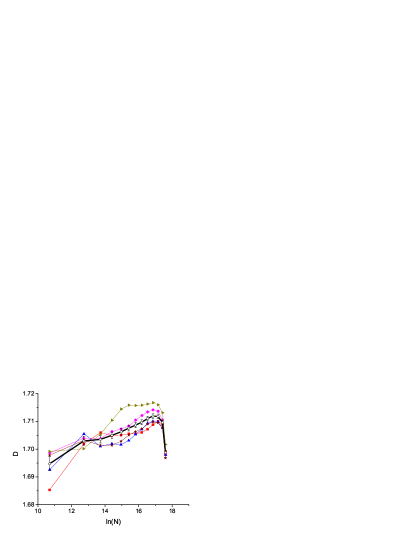
Figure 2: (Color online) Fractal dimension $D(N)$ as a function of the number $N$ of particles inside the radius $R$. Solid curve with error bars represents $D(x)$ averaged over 100 clusters. Another curves are the averages over five different 20-clusters ensembles.

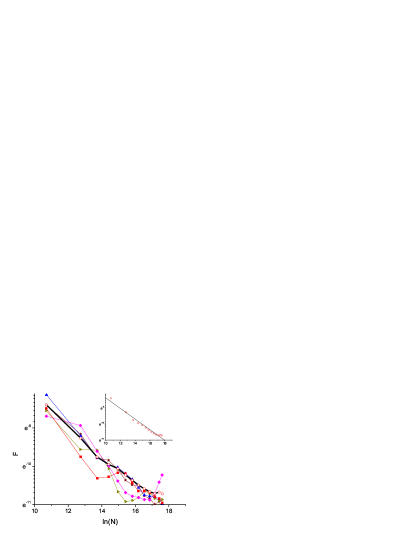
Figure 3: (Color online) Decay of the relative fluctuations of the fractal dimension shown in Figure 2. The symbols are the same as in Figure 2. The solid line in the inset is the linear fit to the open circles.

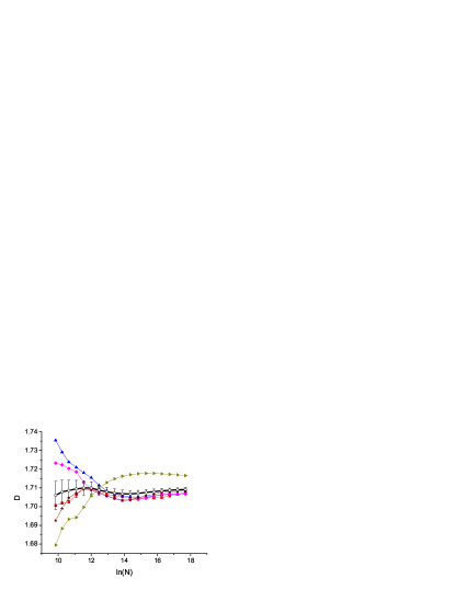
Figure 4: (Color online) Fractal dimension $D_{\rm harm}(N)$ as a function of the number of particles in the cluster used to estimate $R_{\rm dep}$ with averaging over the harmonic measure. The symbols are the same as in Figure 2.

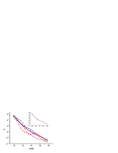
Figure 5: (Color online) Decay of the relative fluctuations of the fractal dimension $D_{\rm harm}(N)$ shown in Figure 4. The symbols are the same as in Figure 2. Inset: the linear fit to the data with $N$ up to $5\cdot 10^{5}$ and the linear fit to the data with larger $N$.

V Multiscaling

It was long discussed that DLA clusters are not simple fractals ms-PZ ; ms-DHOPSS ; ms-CZ ; ms-ACMZ ; ms-Os91 and, for example, that the fractal dimension depends continuously on the normalized distance from the cluster origin ms-ACMZ . It was suggested in ms-ACMZ that the density of particles at a distance $r$ from the origin obeys the equation $g(r,R_{\rm gyr})=c(x)R_{\rm gyr}^{D(x)-d}$, where $x=r/R_{\rm gyr}$, with a nontrivial (non constant) multiscaling exponent $D(x)$ (lines with open symbols in Figure 6).

Quite recently, Somfai et al. nms-BBSS ; nms-SBBS claimed that the multiscaling picture is wrong and is misled by finite-size transients. They argued for a strong dependence of the radius estimators ($R_{\rm dep},R_{2}$, etc., see Table 2) on the system size Expr. (1), where the leading subdominant exponent is estimated as $\nu\approx 0.33$.

It is well known ms-PZ ; Lee ; nms-SBBS that the fractal dimension $D(x)$ can be found using the probability $P(r,N)$ for the N-th particle to be deposited within a shell of width ${d}r$ at a distance $r$ from the seed. The simplest and most obvious form of the probability is $P(r,N)=\frac{1}{\xi(N)}f(\frac{r-R_{\rm dep}(N)}{\xi(N)})$, where $f(y)$ is Gaussian. Practically, the Gaussian distribution can be obtained by averaging over a large number of clusters. For the single-cluster realization this function has some particular form reflecting the details of the cluster growth as shown in Figure 7, in which each local maximum is associated with an actively growing branch.

In nms-SBBS Somfai et al. computed $D(x)$ from the Gaussian probability $P(r,N)$, and $D(x)$ with corrections to scaling coincides well with the numerical results of Amitrano et al. ms-ACMZ . Somfai et all state that $D(x)$ tends to a constant value as $N\to\infty$. In other words, Somfai et al. advocate that multiscaling is transient and is an artifact of the finite size of the DLA clusters.

In contrast, our numerical results demonstrate that (1) there is no evidence for the finite-size corrections with the exponent $\nu=0.33$, (2) $D(x)$ seems not tend to a constant, and (3) it is not correct to use the Gaussian probability $P(r,N)$ to compute $D(x)$ for the DLA model.

Gaussian distribution does not reflect details of the DLA cluster because it is the outcome of the the averaging over a large number of clusters. After such averaging all details of the random nature of the growth of a particular cluster are washed out, and the Gaussian distribution is just the result of the central limit theorem. There are some indications by Hastings Hastings , who computed DLA fractal dimension from field theory, that the Gaussian distribution by itself is insufficient for describing DLA clusters, and some noise must be added to obtain a model corresponding to the DLA model. To some extent, the local maxima in Figure 7 are due to that noise, in contrast to the distribution averaged over the cluster ensemble, which is smooth.

Accordingly, $D(x)$ calculated from the averaged distribution would be constant in the limit of large $N$. We can therefore say that multiscaling comes from the fluctuations (natural noise) of the DLA cluster growth process.

The fractal dimension $D(x)$ for different cluster sizes are shown in Figure 6 together with the results from ms-ACMZ . There is a notable maximum in $D(x)$ at around $x=1.4$, and its size does not change significantly with the number of particles in a cluster. We note that the position of the maximum can be found from the ratio of $(R_{\rm dep}-\xi)$ to $R_{\rm gyr}$. In our simulations, it equals $1.19$, which coincides well with the data in Figure 6.

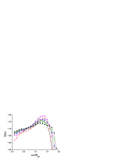
Figure 6: (Color online) Multiscaling fractal dimension D(x) for different cluster sizes: solid triangles, $N=10^{6}$; solid squares, $N=10^{7}$; stars, $N=5\cdot 10^{7}$; solid circles, limit of our data for $N\rightarrow\infty$; open symbols are from ms-ACMZ ; open squares, $N=10^{4}$ square lattice; open circles, $N=10^{5}$ off-lattice.

The maximum seems to occur because growth is mostly completed in the region $r<R_{\rm dep}-\xi$ , and the fractal dimension $D(x)$ decrease to the left of $x=(R_{\rm dep}-\xi)/R_{\rm gyr}$ in the actively growing region $D(x)$ because of the lack of particles there. For small $x$, i.e., for $r<<R_{\rm gyr}$, no new particles are being added, and $D(x)$ is the same for different cluster sizes.

We note that the prediction of Somfai et al. for $D(x)$ with a system size $N=10^{7}$ is quite smaller than the one computed by us and presented in Figure 6. We also estimate limit of the three curves plotted in Fig. 6, taking limit of $N\rightarrow\infty$ at the fixed value of $x$, and plot result with the solid circles in Fig. 6. Thus, our data does not demonstrate tendency of $D(x)$ to a constant value, and rather support our observation that the dynamic growth of the cluster is dominated by the active zone, and maximum in $D(x)$ reflects this nature of DLA. At the same time we have to note that accuracy of the data presented here is not enough for the final decision, and future investigation with the higher accuracy have to be still done.

VI Summary

We have implemented modifications to the DLA algorithm that help us to grow large DLA clusters and test some recent claims about its properties. In our experiments, aggregates do not exhibit corrections to scaling laws. Nevertheless, the results show multiscaling properties. This means that there should be another way for such a clusters to appear. We tried to analyze the processes responsible for multiscaling. We will address this question in future research.

Appendix A Probability to be alive on the birth circle

The main result of this Appendix is expression (7). The same expression was obtained earlier  in Refs. SSZ ; KVMW . We found our result is still worth publishing, since we derive it from a different point of view.

Figure 7: Probability $P(r)$ for a particle to stick at the distance $r$, computed for a single DLA cluster.

We consider a particle at some position $(r;\phi=0)$ outside circle of radius $R_{\rm b}$, $r>R_{\rm b}$. The particle moves randomly, and its size and step is much smaller than $r$ and $R_{\rm b}$. The question is what is the probability for a particle to intersect the circle $R_{\rm b}$ at the angle $\varphi^{\prime}$. Clearly, for the particles walking from infinity, i.e., $r>>R_{\rm b}$, that distribution is uniform in $[-\pi;\pi]$:

$$P(\varphi)d\varphi=\frac{1}{2\pi}d\varphi.$$ (2)

The conformal map

$$w=R_{\rm b}\frac{zr+R_{\rm b}}{r+zR_{\rm b}}$$ (3)

maps infinity to $(r,0)$ and the unit circle to the circle of radius $R_{\rm b}$. Transformation (3) changes probability (2) to the modulus of derivative of the conformal map,

$$\frac{dz}{dw}=\frac{R_{\rm b}^{2}-r^{2}}{R_{\rm b}(r-w)^{2}}.$$ (4)

Substituting $w=R_{\rm b}\exp(i\varphi^{\prime})$ in (4), we obtain the resulting probability

$$P(\varphi^{\prime})=\frac{\rm const}{x^{2}-2x\;\cos\varphi^{\prime}+1}$$ (5)

as a function of the ratio $x=r/R_{\rm b}>1$. This is a probability for the particle beginning its walk at the point $(r,0)$ outside $R_{\rm b}$ to intersect circle $R_{b}$ at the angle $\varphi^{\prime}$ (see Figure 8).

Figure 8: Sketch of probability $P(\varphi^{\prime})$ of the walk intersection of the circle $R_{\rm b}$ with the initial position of the particle at $(r,0)$.

The constant in (5) is associated with the probability for the particle to move to infinity. It can be identified using the analogy between the DLA model and Laplacian growth as was pointed in Pietronero for the dielectric breakdown model, which is a generalization of the DLA model.

The probability that the particle sticks somewhere to the cluster is proportional to the electrical field at that point. We consider three circles of radii $R_{1}$, $R_{2}$, and $R_{3}$, $R_{1}<R_{2}<R_{3}$. The external circles $R_{1}$ and $R_{3}$ are set under the potential $\Phi=0$, and particles stick one of them. The circle $R_{2}$ (place of a birth for particles) is set with $\Phi=1$. The solution of the Laplace equation $\nabla^{2}\Phi=0$ with the above boundary conditions gives the distribution of the potential and thus of the electrical field $\bf{E}$. The probability for the particle to stick on the circle $R_{1}$ would be $P_{1}=\rm{const}*\int_{|r|=R_{1}}|\bf{E}|\,{d}^{2}r$ and similarly for $P_{3}$. The ratio of these probabilities is:

$$\frac{P_{3}}{P_{1}}=\frac{\log\frac{R_{2}}{R_{1}}}{\log\frac{R_{3}}{R_{2}}}$$ (6)

The probability $P_{3}$ vanishes as $R_{3}\to\infty$: $P_{3}\to 0$. This means that all particles starting on the birth radius should irreversibly collide with a cluster and the constant in (5) is easily found by normalizing the probability, $\rm{const}=(x^{2}-1)/2\pi$. The final expression for the probability

$$P(\varphi^{\prime})=\frac{1}{2\pi}\frac{x^{2}-1}{x^{2}-2x\;\cos\varphi^{\prime}+1}$$ (7)

provides correct values for both the limits $x\to\infty$ and $x\to 1$. The same expression for probability was described in SSZ , but it was obtained other way. Transformation

$$f(u)=2\arctan\left(\frac{x-1}{x+1}\tan(u\pi/2)\right)$$

maps uniformly distributed in interval $[-1,1]$ random number $u$ to random number with distribution (7).

Appendix B Memory organization

Step 3 of the algorithm described in Section II essentially contains two routines. We must choose, first, the direction of the random walk and, second, the walk length. The direction of the walk is chosen uniformly in $[0;2\pi]$. Because the motion is uniform in direction, we can increase the step, but only if particle is far away from the cluster (in our simulations we choose that distance such that particle is more than five units away from the cluster, otherwise, its step is one unit of length). The length for the big step is chosen with the condition that the walk should not intersect any particles of the cluster. Therefore, the distance to the cluster $d_{\rm pc}$ is evaluated, and the step length is taken as that distance.

The reason for implementing variable step length is as follows. Most of the time the particle is moving far away from the cluster, and choosing a step length of the order of the particle distance from the cluster accelerates simulations.

To realize all the proposed improvements efficiently we must organize memory in a special manner. When the particle moves, we must know whether it collides with a cluster, and to check this, we must iterate over all particles. Such an approach is rather unreasonable and we must therefore restrict the number of particles to test. This is easily done by dividing the space into square cells, each about twenty units of length. Each cell saves information about particles that stuck in the region covered by it. We therefore need only check cells that are in the region of one step.

This model also improves the process of seeking the size of free space for the big step. To find the distance from current position to the cluster precisely is a difficult task, but it suffices in most cases to know it with an accuracy estimated from below, the size of one cell. Figure 9 shows how this is done. Cells are plotted in the picture as squares with bold lines. They are marked with numbers showing their distance from the particle location. For simplicity, cells with the same number are thought to be at the same distance from the particle. Occupied cells are shaded. In this example the particle is allowed to jump with the step length $L-2R$, where $L$ is the cell size, and $R$ the particle radius. The distance $L$ is the radius of the inscribed circle with a center somewhere in cell $0$ (in the worst case, the center lies on the border of cell $0$). This length should be reduced because cells save only particle centers and there could be a projection of a particle into another cell with a size of $R$. To simplify the algorithm we seek the step length only using the free/occupied cells picture. The first step is to check whether there are other particles in the cell we are now in, then we should check cells marked with 1, then marked with 2 (not shown in picture), and so on until we find an occupied cell.

During DLA growth, the intervals between branches increase notably, and the time to traverse all cells while seeking an occupied one also increases. To reduce the influence of such a process, Ball and Brady BB-alg developed a hierarchical memory model, where one cell is divided into smaller subcells and so on. This approach seems rather memory consumptive: in growing a large cluster, it would become a bottleneck of an algorithm.

The desired effect can be achieved in another way. Because the cell size is much more bigger than the particle size, the distribution of free cells changes slowly, and process of seeking the maximum free space could be started not from the particle position but from the free line achieved in the previous search from this origin. To implement this we must save the value of free space around each cell. If this information is unknown, i.e., it is the first time to seek the maximum step length from the current cell, we should traverse all cells from the beginning; otherwise we start from the line previously saved and move to the center.

The cell size is chosen as follows. It should not be very small: a small size results in high memory consumption and a rapid change of the distribution of free cells. On the other hand, its size restricts the precision of the length we find for the big step, i.e., there is a region of cell size near the cluster where particles can move only with a small steps. To avoid this last constraint, we use second-layer information. Like Ball and Brady, we divide the cells into smaller ones. To minimize memory consumption, we realize them as an 32 bit integer, where each bit shows whether the corresponding subcell is occupied. Each big cell can therefore be divided into not more than 25 subcells.

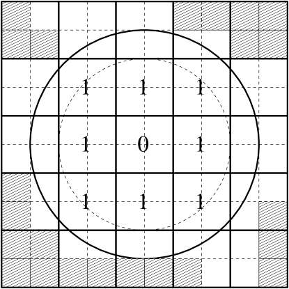
Figure 9: Determination of the step length.

As mentioned above, the second-layer information is only used when the particle moves near the cluster, where the accuracy given by the first layer is insufficient. Figure 9 shows large cells (bold borders) and small cells. Using the first layer we can find that only the space inside the dashed circle is free. The second layer gives a more precise result: the particle can jump up to the bold circle.

References

- (1) T.A. Witten and L.M. Sander, Phys. Rev. Lett. 47 (1981) 1400.
- (2) A. Bunde and S. Havlin, eds., Fractals and Disordered Systems (Springer, Berlin, 1996).
- (3) M.B. Hastings and L.S. Levitov, Physica D 116 (1998) 244.
- (4) M.B. Hastings, Phys. Rev. E 55 (1997) 135.
- (5) P. Meakin, H.E. Stanley, A. Coniglio, T.A. Witten, Phys. Rev. A 32 (1985) 2364.
- (6) T.C. Halsey, P. Meakin, and I. Procaccia, Phys. Rev. Lett. 56 (1986) 854.
- (7) T.C. Halsey, B. Duplantier, and K. Honda, Phys. Rev. Lett. 78 (1997) 1719.
- (8) M. Plischke and Z. Rácz, Phys. Rev. Lett. 53 (1984) 415.
- (9) B. Davidovitch, H.G.E. Hentschel, Z. Olami, I. Procaccia, L.M. Sander, and E. Somfai, Phys. Rev. E 59 (1999) 1368.
- (10) A. Coniglio and M. Zannetti, Physica A 163 (1990) 325.
- (11) C. Amitrano, A. Coniglio, P. Meakin, and M. Zannetti, Phys. Rev. B 44 (1991) 4974.
- (12) P. Ossadnik, Physica A 176 (1991) 454, ibid. 195 (1993) 319.
- (13) R.C. Ball, N.E. Bowler, L.M. Sander, E. Somfai, Phys. Rev. E 66 (2002) 026109.
- (14) E. Somfai, R.C. Ball, N.E. Bowler, L.M. Sander, Physica A 325 (2003) 19.
- (15) R.C. Ball and R.M. Brady, J. Phys. A 18 (1985) L809.
- (16) E. Sander, L. M. Sander, R. M. Ziff, Computers in Physics 8 (1994), 420-425; L.M. Sander, Contemporary Physics 41 (2000), 203-218.
- (17) H. Kaufman, A. Vespignani, B.B. Mandelbrot, and L. Woog, Phys. Rev. E 52 (1995) 5602.
- (18) L. Niemeyer, L. Pietronero, H.J. Wiesmann, Phys. Rev. Lett., 52 (1984) 1033.
- (19) P. Meakin, J. Phys. A 18 (1985) L661.
- (20) P. Meakin, L.M. Sander, Phys. Rev. Lett. 54 (1985) 2053.
- (21) J. Lee, S. Schwarzer, A. Coniglio, H.E. Stanley, Phys. Rev. E 48 (1993) 1305.
- (22) S. Tolman and P. Meakin, Physica A 158 (1989) 801; Phys. Rev. A 40 (1989) 428.
- (23) T.A. Rostunov and L.N. Shchur, JETP 95 (2002) 145.