Synchronizability and synchronization dynamics of weighed
and unweighed scale free networks with degree mixing

Abstract

We study the synchronizability and the synchronization dynamics of networks of nonlinear oscillators. We investigate how the synchronization of the network is influenced by some of its topological features such as variations of the power law exponent $\gamma$ and the degree correlation coefficient $r$. Using an appropriate construction algorithm based on clustering the network vertices in $p$ classes according to their degrees, we construct networks with an assigned power law distribution but changing degree correlation properties. We find that the network synchronizability improves when the network becomes disassortative, i.e. when nodes with low degree are more likely to be connected to nodes with higher degree. We consider the case of both weighed and unweighed networks. The analytical results reported in the paper are then confirmed by a set of numerical observations obtained on weighed and unweighed networks of nonlinear Rössler oscillators. Using a nonlinear optimization strategy we also show that negative degree correlation is an emerging property of networks when synchronizability is to be optimized. This suggests that negative degree correlation observed experimentally in a number of physical and biological networks might be motivated by their need to synchronize better.

Keywords: Complex Network, Synchronization

1 Introduction

Networks of oscillators abound in physics, biology and engineering. Examples include communication networks, sensor networks, neuronal connectivity networks, biological networks and food webs [?]. Under certain conditions such networks are known to synchronize on a common evolution, with all the oscillators exhibiting the same asymptotic trajectory. Synchronization was observed to play an important role in a wide variety of different problems (physical, ecological and physiological networks to name just a few); see for example [?, ?, ?, ?, ?, ?, ?, ?].

In this paper, we consider a network consisting of $N$ identical oscillators coupled through the edges of the network itself [?, ?]. We suppose each oscillator is characterized by its own dynamics, $x(t)=\{x_{i}(t),i=1...N\}$, described by a nonlinear set of ODEs, $\dot{x}=f(x)$. The dynamics of each oscillator in the network is perturbed by the output function of its neighbors represented by another nonlinear term, say $h=h(x)$. The equations of motion for each oscillator can then be given as follows:

$$\frac{dx_{i}}{dt}=f(x_{i})-\sigma\sum_{j=1}^{N}{\mathcal{L}}_{ij}h(x_{j}),\qquad i=1,2,...N,$$ (1)

where $\sigma$ represents the overall strength of the coupling. Note that information about the network topology is entirely contained in the matrix $\mathcal{L}$, whose entries $\mathcal{L}_{ij}$, $j\neq i$, are negative (zero) if node $i$ is (not) connected to node $j$, with $\mid\mathcal{L}_{ij}\mid$ giving a measure of the strength of the interaction.

In recent years, the analysis of large sets of data led to the identification of some important structural properties of many real-world networks; see for a review [?]. Among these, the degree distribution $P(k)$, with the degree $k$ being the number of connections at a given node, was shown to be one of the most important features. In particular, scale-free networks, which are characterized by a power law degree distribution $P(k)\sim k^{-\gamma}$, have been observed to be widely spread in nature [?], [?]. The main feature of scale free networks is an high heterogeneity in the degree distribution (higher than in purely random networks). Heuristically, this corresponds to the fact that real networks have often many low-degree nodes and only few nodes, termed as hubs, with many connections (thus leading to the high heterogeneity in the degree distribution). Such a characterization is particularly relevant since it has been shown to have important effects on the dynamics occurring over the network, such as the spreading of epidemics [?], [?] or the distribution of packets in traffic dynamics over the network [?], [?], [?]. Also, it was shown that the scale-free structure of a network can have an important effect on its synchronizability (see Sec. 2 for further details).

Recently, it has been suggested that real networks can often exhibit other important features. For instance, in the real world, nodes are not only abstract objects without any attribution, but each of them is characterized by some intrinsic features. Examples of interest could be the vertices age, spatial location, functional importance, level of activity and the number of connections each vertex has (that is the degree). An important topological property of physical and biological networks is that often their nodes show preferential attachment to other nodes in the network according to their degree [?], [?]. Networks are said to exhibit assortative mixing (or positive correlation) if nodes of a given degree tend to be attached with higher likelihood to nodes with similar degree. (Similarly disassortative networks are those with nodes of higher degree more likely to be connected to nodes of lower degree.)

The presence of correlation has been detected experimentally in many real-world networks. Interestingly, from the analysis of real networks, it was noticed that social networks are characterized by positive degree correlation, while physical and biological networks show typically a disassortative structure [?]. For example, in [?], Internet was found to exhibit disassortative mixing at the Autonomous System level.

In mathematical terms, degree correlation can be quantified by means of the observable $r$, introduced in [?] and [?]. In particular, the coefficient $r$ was proposed in [?] as a normalized measure of degree correlation, defined as the Pearson statistic:

$$r=\frac{\sum_{ij}ij(e_{ij}-q_{i}q_{j})}{{\sigma_{q}}^{2}},$$ (2)

where $q_{k}$ is the probability that a randomly chosen edge is connected to a node having degree $k$, $\sigma_{q}$ is the standard deviation of the distribution $q_{k}$ and $e_{ij}$ represents the probability that two vertices at the endpoints of a generic edge have degree $i$ and $j$ respectively.

The main aim of this paper is to investigate the relationship between the presence of degree correlation and the network synchronizability properties. Specifically, we shall seek to characterise how the presence of correlation on the network affects the synchronizability of the nonlinear oscillators at the nodes. We will show that correlation has indeed an effect on synchronizability in both weighed and unweighed networks. Our main finding is that disassortative networks synchronize better. Thus, as will be further discussed in the paper, the presence of negative degree correlation often detected in technological and particularly biological networks of nonlinear oscillators might be motivated by its benefits in terms of the network synchronizability.

The rest of the paper is organised as follows. In Sec. 2 we briefly review the Master Stability Function approach and the effects on synchronizability of heterogeneity in the degree distribution, which is typical of scale free networks. In Sec. 3, we analyze how degree correlation can influence the synchronizability of unweighed networks and give an analytical explanation of the observed phenomena. Also, an optimization approach is used to motivate the conjecture that negative degree correlation can be an emerging property of networks when the aim is to optimize their synchronization. The case of weighed networks is discussed in Sec. 4, while the study of synchronization of both weighed and unweighed networks of Rössler oscillators is presented in Sec. 5.

2 Effects of Topology on the Network Synchronizability

2.1 The Master Stability Function Approach

Recently, it has been proposed that the network topology, i.e. the way in which the oscillators are mutually coupled among themselves, has an important effect on the network synchronizability. This is defined in terms of the linear stability of the synchronous equilibrium ($x_{i}=x_{2}=...=x_{N}=x_{s}$), whose existence is guaranteed by the fact that ${\mathcal{L}}$ is a zero row-sum matrix.

The stability of the synchronization manifold can be investigated by perturbing trajectories lying on it along directions which are orthogonal to the manifold itself. Namely, we consider sufficiently small perturbations $\epsilon_{i}$ from the synchronous state so that $x_{i}(t)=x_{s}(t)+\epsilon_{i}(t)$, and:

$$\frac{d\epsilon_{i}}{dt}=Jf(x_{s})\epsilon_{i}-\sigma\sum_{j=1}^{N}{\mathcal{L}}_{ij}Jh(x_{s})\epsilon_{j},$$ (3)

where $J$ denotes the Jacobian matrix. Following the strategy presented in [?], Eq. (3) can be transformed in blocks of the form:

$$\frac{d\eta}{dt}=[Jf(x_{s})-\sigma\lambda_{i}Jh(x_{s})]\eta,\quad i=1,2,...,N$$ (4)

where $\eta$ is defined in [?] in terms of the perturbations $\epsilon_{i}$, $\lambda_{i}$ are the real eigenvalues of the coupling matrix $\mathcal{L}$, ordered in such a way that $\lambda_{1}\leq\lambda_{2}...\leq\lambda_{N}$ (in this manuscript we will deal only with real eigenvalues of the matrix $\mathcal{L}$, although under general conditions, there may be complex conjugate eigenvalues). Note that $\lambda_{1}$ is structurally equal to 0, as the corresponding eigenvector is associated to the mode lying within the synchronization manifold. It is worth observing that using (4), the problem of studying the stability of a generic complex network in (1) has been replaced by that of considering the stability of $N$ simpler independent systems.

This approach is used in [?] to derive the so-called Master Stability Function (MSF). Specifically, eq. (4) is considered as a parametric equation in a parameter $\alpha$, given by:

$$\frac{d\eta}{dt}=[Jf(x_{s})-\alpha Jh(x_{s})]\eta$$ (5)

and the values of $\alpha$ are sought corresponding to the maximum Lyapunov exponent of the system in (5) being negative.

Interestingly, it can be shown that for a broad class of systems (associated to different dynamic functions $f$ and output functions $h$ ), the Master Stability Function is negative in a bounded range of the parameter $\alpha$, say [$\alpha_{min},\alpha_{max}$].

Thus, in order to guarantee the stability of the synchronization manifold, all the $\sigma\lambda_{i}$, for $i=2,3,...,N$, must lie in the range [$\alpha_{min},\alpha_{max}$]. Simply, this condition reduces to the following:

$$\sigma\lambda_{2}>\alpha_{min}\qquad\sigma\lambda_{N}<\alpha_{max},$$ (6)

or equivalently, to:

$$\frac{\lambda_{N}}{\lambda_{2}}<\frac{\alpha_{max}}{\alpha_{min}},$$ (7)

which guarantees the existence of at least one value of $\sigma$, for which the synchronization manifold is stable. Note that while $\alpha_{max}$ and $\alpha_{min}$ are completely determined by assigning the functions $f$ and $h$, $\lambda_{N}$ and $\lambda_{2}$ depend solely on the network topology. Thus, the synchronizability of a given network can be defined independently from the functional form of the dynamical systems at its nodes (i.e. of the functions $f$ and $h$).

In general, (6) defines a bounded range of values of $\sigma$, say $I_{\sigma}=[\frac{\alpha_{min}}{\lambda_{2}},\frac{\alpha_{max}}{\lambda_{N}}]$, for which synchronization is attained. Therefore, an increase of $\lambda_{2}$ and a decrease of $\lambda_{N}$ can lead to a larger interval $I_{\sigma}$. Thus, minimizing the eigenratio $R=\lambda_{N}/\lambda_{2}$ yields a broadening of the range of values of $\sigma$ over which the network synchronizes.

Using the MSF approach, it is possible to investigate the effects on synchronization of the structural properties of the network topology (in terms of the eigenratio $\lambda_{N}/\lambda_{2}$). Hence, it is meaningful to characterise how the network topological features affect the Laplacian eigenratio.

2.2 Synchronizability of Scale-free networks

Sofar, the effects of the network topology on its synchronizability have been studied mainly with respect to the presence of scale free topologies or patterns in the network; see for example, [?], [?], [?], [?], [?], [?], [?], [?, ?].

Scale free networks, which are common in nature, were found to show better synchronizability for increasing values of the power law exponent in [?], [?]. Specifically, the relationship was analyzed between the network structure and its synchronizability. An interesting phenomenon was observed which was termed as the ”paradox of heterogeneity”; specifically, although heterogeneity in the degree distribution leads to a reduction in the average distance between nodes (the so called small world effect [?]), it may suppress synchronization.

To explain the observed phenomena, in [?], the transition of the underlying network from scale free (power law distributed) to random (Poisson distributed) was shown to have a big impact on the eigenratio $R$ of the Laplacian eigenvalues. Namely, a decrease of the heterogeneous nature of the network was discovered to yield, as a result, a reduction of $R$, thus increasing the synchronizability of the network itself.

3 Effects of degree correlation on the Laplacian eigenratio

In [?], we proposed that a further decrease of $R$ can be detected when negative degree correlation is introduced among the network nodes. Specifically, in [?], using the configuration model [?], disassortative networks were found to synchronize better. In this section, we start by extending some of the results presented therein to the case of unweighed networks constructed by using the static model, which was firstly introduced in [?].

3.1 Network Construction methodology

In this paper, in order to construct networks characterized by a given degree distribution, we will use the following algorithm:

1. We associate to each vertex $i=1...\mathcal{N}$ a weight or fitness $\phi_{i}\propto(i+\theta)^{-\alpha}$, with $\alpha=[0,1)$, $\theta$ being a fixed parameter.

2. Then, links are added among the network nodes with probability proportional to the vertices weights, until $\mathcal{E}$ links have been introduced.

Note that by using this methodology, the expected degree at each node $i$, is $k_{i}\simeq\phi_{i}\mathcal{E}$, and it can be shown that the degree distribution is expected to follow a power law, $P(k)\sim k^{-\gamma}$, with $\gamma={{1+\alpha}\over{\alpha}}$.

Observe that the nodes fitness $\phi_{i}$, is the only parameter of the model; we wish to emphasize that assigning the fitness corresponds to assigning the expected degree at the vertices, thus the degree at the nodes can be considered as an equivalent parameter of the model.

By using such a model, the giant component of the network may not include all the network nodes, i.e the number of connected nodes, say $N$, may be $\leq\mathcal{N}$. In Fig. 1, $N/{\mathcal{N}}$ has been plotted as varying both $\gamma$ and $r$. In what follows, we will consider only the largest connected part of each generated network and refer to $N$ as the number of nodes belonging to the giant component.

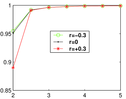
Figure 1: $N/\mathcal{N}$ as varying the degree distribution exponent $\gamma$ in networks characterized by different values of the degree correlation coefficient $r$. The legend is as follows: $r=-0.3$ (o), $r=0(\cdot)$, $r=+0.3(\triangle)$. $\mathcal{N}=10^{3}$ nodes, $\mathcal{E}=4\cdot 10^{3}$, $\theta=10$.

Using this methodology to construct a network, we can handle the transition from very heterogenous scale free networks (when $\alpha=1$ and $\gamma=2$), to highly homogenous ones (as $\alpha$ approaches 0 and $\gamma$ approaches $\infty$); note that in the limit of $\gamma\rightarrow\infty$, in which to each vertex is associated the same weight, we recover the classical random network model, which was introduced in [?]. Moreover, this does not imply a dependence of the total number of edges on the degree distribution exponent $\gamma$ (as is the case of the widely used configuration model [?]).

By using this model we are able to reproduce networks characterized by: (i) a given number of nodes $N$, (ii) a desired number of edges $\mathcal{E}$, (iii) a degree distribution with a desired value of the exponent $\gamma$ (note that the same model has been already employed to study the synchronization properties of networks in [?] and in [?].) Then it is possible to devise a strategy similar to the one presented in [?], to generate networks with a given level of assortativity, i.e. a desired value of the degree correlation coefficient $r$.

Notice that the model introduced in [?] is known to exhibit spontaneous negative degree correlation [?] when $2<\gamma<3$ (this phenomenon being referred to in [?] as a fermionic constraint, due to the impossibility of connecting pairs of nodes with more than one link). The same phenomenon has been observed also in networks constructed by using the configuration model, as described in [?, ?, ?]. However, in what follows, we will disregard this particular effect; namely, we will compare networks characterized by different degree correlation properties according to the values of the index $r$ (including the case $r=0$), which have indeed been measured over the networks.

3.2 Unweighed networks

In the rest of this section we will investigate the case of unweighed network topologies, with all the links being associated to a constant unitary weight. Specifically in such a case, the matrix $\mathcal{L}$ can be written as follows:

$$\mathcal{L}=D-A,$$ (8)

where $D=\{D_{ij}\}$ is a diagonal matrix such that $D_{ii}=k_{i}$, $i=1,2,...,N$, and $A$ is the associated adjacency matrix. The case of weighed topologies will be considered in Sec. 4.

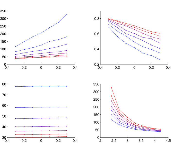
Figure 2: Synchronizability of degree correlated scale free networks of size $10^{3}$nodes. Behavior of the eigenratio $\lambda_{N}/\lambda_{2}$ (a), of the second lowest eigenvalue $\lambda_{2}$ (b) and of the highest one $\lambda_{N}$ (c), as functions of the correlation coefficient $r$ defined in [11], for $\gamma$ varying from 2.4 (top line) to 4.2 (bottom line) in steps of 0.3. (d) The eigenratio as function of $\gamma$ as varying the correlation coefficient $r$ from $-0.3$ (bottom line) to $0.3$ (top line) in steps of $0.1$. The lines are guided by the eye.

The overall results are summarized in Fig. 2(a) where the effects of varying the degree correlation on the Laplacian eigenratio $R$ are shown for different values of the degree distribution exponent $\gamma$. As discussed in [?], in the case of uncorrelated networks ($r=0$), synchronizability improves for increasing values of $\gamma$. Moreover, for all values of $\gamma$, we observe a reduction of $R$ for decreasing values of $r$. This means that disassortative mixing enhances the network synchronizability. Interestingly, as depicted in Fig. 2(b) and Fig. 2(c), we observe that, under variations of the correlation parameter, the changes in $R$ seem to be mainly due to variations of $\lambda_{2}$. This is not surprising if we consider that $\lambda_{N}$ is known to scale with $k_{max}$ [?], the maximum degree at the vertices and $k_{max}$ cannot vary with the degree correlation coefficient $r$.

It is worth noting here that the results provided in this section are obtained by using a different network generation model from that used in [?]. Moreover, the results shown in this paper (and in particular those in Fig. 2) are found to confirm those previously presented therein.

3.3 An analytical explanation

Here we briefly expound in this context the analysis provided in [?], in order to provide an explanation of the behavior of the eigenratio $R$ as a function of the degree correlation coefficient $r$ depicted in Fig. 2.

Suppose the network vertices are divided in $p$ classes according to their degree, i.e. clustering in each class ${\mathcal{C}}_{i}$ all the vertices having degree $k_{i}$, ($i=1,2,...p$). Let us term as $n_{i}$ the number of vertices in class ${\mathcal{C}}_{i}$, then the probability of finding a vertex belonging to class ${\mathcal{C}}_{i}$ at the end of a randomly chosen edge within the network is given by $q_{i}=n_{i}k_{i}/\sum_{i}n_{i}k_{i}$. In so doing, following [?], the presence of degree correlation can be estimated by using the coefficient $r$ defined as:

$$r=\frac{{\mathbf{k}}^{T}({\mathbf{E}}-{\mathbf{q}}{\mathbf{q}}^{T})\mathbf{k}}{{\sigma^{2}_{q}}},$$ (9)

where $\sigma_{q}$ is the standard deviation of the distribution $q_{i}$, ${\mathbf{k}}={({k_{1},k_{2},...,k_{p}})^{T}}$, ${\mathbf{q}}={({q_{1},q_{2},...,q_{p}})^{T}}$ and ${\mathbf{E}}=\{e_{ij}\}\in{\mathbb{R}}^{{p}\times{p}}$, with $e_{ij}$ being the probability that a randomly chosen edge in the network connects nodes having degree $i$ and $j$.

From (9), it is possible to obtain the distribution of edges among the network vertices as a function of $r$ as follows:

$${\mathbf{E}}={\mathbf{q}\mathbf{q^{T}}}+{r}{\sigma^{2}_{q}}\mathbf{M},$$ (10)

where $\mathbf{M}$ is a symmetric matrix having all row sums equal to zero and appropriately normalized such that $\mathbf{k^{T}}\mathbf{M}\mathbf{k}=1$. Specifically, we can express ${\mathbf{M}}$ as follows:

$${\mathbf{M}}=\frac{{\mathbf{m}\mathbf{m}}^{T}}{({\mathbf{k}}^{T}{\mathbf{m}})^{2}},$$

where ${\mathbf{m}}={({m_{1},m_{2},...,m_{p}})^{T}}$ is a vector such that $\sum_{i}m_{i}=0$ (for instance we can choose $m$ such that $m_{i}\leq m_{i+1}$ for $i=1,2...,p-1$ in order to have a convenient form of the matrix $\mathbf{M}$ with positive values near the main diagonal and negative values far away from it).

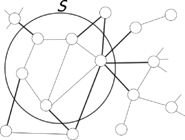
Figure 3: The isoperimetric problem consists in finding the subset $S$ such as to minimize the ratio $h_{G}(S)$ in Eq. (11). In this schematic picture, a given subset S is selected as the set of all network vertices contained inside the circle in the figure. Its cardinality is given by the number of nodes in the circle, $|S|=5$ and its boundary is given by the number of edges (represented in bold) which connect the subset $S$ to the rest of the network, $\mathcal{D}(S)=9$.

As $\lambda_{N}$ is found to be almost independent from the correlation coefficient $r$ (see Fig.1(c)), we will focus now on estimating the effects of correlation on the eigenvalue $\lambda_{2}$, the parameter known as algebraic connectivity of graphs [?]. Specifically, to estimate an upper bound for $\lambda_{2}$, we use the following Cheeger inequality from graph theory [?]:

$$\lambda_{2}\leq h_{G},$$ (11)

with $h_{G}$, the Cheeger constant of a graph, defined as follows [?]:

$$h_{G}=\min_{S}h_{G}(S).$$ (12)

For a given subset of vertices, say $S$, $h_{G}(S)$ is the quantity given by:

$$h_{G}(S)=\frac{{\mathcal{D}}(S)N}{|S|(N-|S|)},$$ (13)

where ${\mathcal{D}}(S)$ is the number of edges in the boundary of $S$ and $|S|<\frac{N}{2}$, is the number of vertices in $S$.

The problem of finding $h_{G}$, known as the isoperimetric problem in graph theory, is illustrated by means of a representative example in Fig. 3. Note that, given a graph of order $N$, there are $\sum_{i=1}^{N/2}C(N,i)$ possible ways of choosing the subset $S$, where $C(a,b)$ is the number of combinations of $a$ elements in $b$ places, and thus the problem of choosing $S$ such as to minimize $h_{G}(S)$ is NP-hard.

We will show that (11) can be successfully used to compute an upper bound on $\lambda_{2}$. To overcome the limitations due to the computation of the subset $S$ that minimizes $h_{G}(S)$, we will follow a stochastic approach in order to estimate $h_{G}(S)$, starting from the available information we have on the network. We will assume that the noticeable features of the network are only the degree distribution and the correlation specified; all other aspects being completely random.

Note that, by considering as equivalent all the vertices characterized by the same degree, the original problem in Fig. 3, can be converted in the other (simpler) one shown in Fig. 4. In the picture, the subset $S$ includes two vertices of degree $3$, two vertices of degree $4$ and one vertex of degree $7$. In terms of the nodes degrees the original problem, consisting of finding the optimal set of vertices, can then be re-interpreted as that of finding the optimal mix of degrees of nodes in $S$.

Figure 4: The problem described in Fig.2 has been converted in the one represented in this picture. Here, the subset $S$ is identified by the degrees of the vertices inside it, which are two nodes of degree $3$, two nodes of degree $4$ and one node of degree $7$. Note that, in the original formulation, the problem was of choosing the vertices to be included in $S$ in order to minimize $h_{G}(S)$. Here we have restated it by considering only the degrees of the vertices to be included in $S$, in terms of the vector $\bf{y}$, such as to minimize $h_{G}({\bf y})$.

Then, we can give a full characterization of a randomly chosen subset $S$ in terms of the number of nodes in it, say $x_{i}$, belonging to each class ${\mathcal{C}}_{i}$ ($i=1,2...,p$). Let us term as $y_{i}=\frac{x_{i}}{n_{i}}$ the fraction of nodes in $S$ drawn from each class ${\mathcal{C}}_{i}$ ($i=1,2...,p$). Then problem (12) becomes that of finding the combination ${\mathbf{y}}={({y_{1},y_{2},...,y_{p}})^{T}}$ such as to minimize $h_{G}({\bf y})$, i.e. $\min_{\bf y}h_{G}({\bf y},r)$. Then, since under this formulation nodes with the same degree are all clustered in the same class, the complexity of the problem is reduced to approximately $\sum_{i=1}^{N/2}C(N,i)/\Pi_{j=1}^{k_{max}}n_{j}$. It is also worth noting here that the subset $S$ is not supposed to satisfy any particular condition, not even of being connected.

Now, we observe that the number of edges in the boundary, say ${\mathcal{D}}(S)$, is given by the total number of edges starting from the vertices in $S$, less the ones, say ${\mathcal{I}}(S)$, that are contained in $S$, i.e. having both endpoints in $S$. Thus we can estimate $\mathcal{I}$ and ${\mathcal{D}}$ as follows:

$${\mathcal{I}}(S)={\mathcal{I}}({\mathbf{y}},r)={\mathcal{E}}{\mathbf{y}}^{T}E\mathbf{y},$$

$${\mathcal{D}}(S)={\mathcal{D}}({\mathbf{y}},r)={\mathbf{x}}^{T}{\mathbf{k}}-2{\mathcal{I}}(S)={2\mathcal{E}(\mathbf{y}}^{T}{\mathbf{q}}-{\mathbf{y}}^{T}E\mathbf{y}),$$

where ${\mathbf{x}}={({x_{1},x_{2},...,x_{p}})^{T}}$ and $\mathcal{E}$ is the total number of edges in the network.

Therefore $h_{G}(S)$ becomes:

$$h_{G}({\mathbf{y}},r)=\frac{{2\mathcal{E}(\mathbf{y}}^{T}{\mathbf{q}}-{\mathbf{y}}^{T}E{\mathbf{y}})N}{({\mathbf{n}}^{T}{\mathbf{y}})(N-{\mathbf{n}}^{T}{\mathbf{y}})},$$ (14)

under the constraint that ${\mathbf{n}}^{T}{\mathbf{y}}<N/2$, where ${\mathbf{n}}$ is the vector $({n_{1},n_{2},...,n_{p}})^{T}$. A numerical optimization algorithm can then be used to find the subset $S$ that minimizes $h_{G}(\mathbf{y},r)$ in terms of $y_{1},y_{2},...,y_{p}$ (and subsequently $r$) and, in turns, an upper bound for $\lambda_{2}$.

Also, from (10) and (14), we get:

$$\frac{\partial{h_{G}(S)}}{\partial{r}}\propto\frac{\partial{{\mathcal{D}}(S)}}{\partial{r}}=-2{\mathcal{E}}\sigma^{2}_{q}{({\mathbf{y}}^{T}\mathbf{m})}^{2}\leq 0.$$ (15)

Since, for any vector $\mathbf{y}$, (15) is satisfied, then we have that $\frac{\partial{h_{G}}}{\partial{r}}\leq 0$. Therefore, we can predict analytically that $h_{G}$ and hence $\lambda_{2}$ will be decreasing as the degree correlation is increased and, as a consequence, the eigenratio $\lambda_{N}\over\lambda_{2}$ will increase for higher values of the correlation coefficient.

Another interesting inequality in spectral geometry is due to Mohar [?]:

$$\lambda_{2}\geq k_{max}-\sqrt{{k_{max}}^{2}-{h^{\prime}_{G}}^{2}},$$ (16)

where $h^{\prime}_{G}=\min_{S}{\frac{{\mathcal{D}}(S)}{|S|}}={2\mathcal{E}(\mathbf{y}}^{T}{\mathbf{q}}-{\mathbf{y}}^{T}E{\mathbf{y}})/({\mathbf{n}}^{T}\mathbf{y})$. Using (16), we can also get a lower bound on $\lambda_{2}$. Then following an approach similar to the one used to compute the upper bound, it is easy to show that the lower bound in (16) has to decrease with $r$ (note that when making the correlation change, the degree distribution is fixed and thus, $k_{max}$ cannot vary with $r$). Since both the upper and the lower bounds have to decrease with $r$, $\lambda_{2}$ is also expected to have the same trend.

3.4 Disassortativity as an emerging property

The main result of the derivation presented above is the finding that disassortative networks synchronize better. We wish now to assess whether negative degree correlation can be thought of as an emerging property of networks with an assigned degree distribution in order to improve their synchronization. In particular, we noticed that the variation of the degree correlation affects mainly the Laplacian eigenvalue $\lambda_{2}$. Thus, we shall seek to find if varying the correlation, while keeping the degree distribution fixed, is indeed a good way of optimizing the network synchronizability properties.

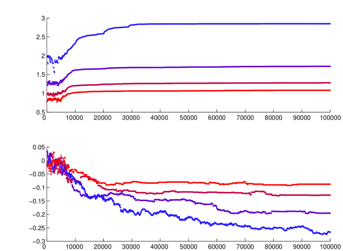
Figure 5: Effects of the maximization of $\lambda_{2}$ on the correlation parameter $r$ defined in [11] for different scale-free networks with $\gamma=[2,3,4,5]$.

This might be a solution to a classical problem in graph theory optimization which is the construction of expander graphs, i.e. highly efficient communication networks, characterized by high values of $\lambda_{2}$ [?] (and therefore low values of the eigenratio $R$).

We will use a simulated annealing meta-heuristic technique, to solve the problem of maximizing $\lambda_{2}$ while keeping unchanged the network degree distribution. To this aim, given a network with a certain degree distribution, we will perform the following iterative procedure. At each step, the endpoints of a randomly selected pair of edges are exchanged if $\exp{(\frac{-\Delta(\lambda_{2})}{T})}>z$, where $z$ is an uniformly distributed random variable between 0 and 1, $\Delta(\lambda_{2})$ is the variation achieved in the objective function $\lambda_{2}$ before and after the execution of the move and $T$ is a control parameter, which similarly to the original formulation of the simulated annealing procedure is known as the system ’temperature’. As the algorithm runs, the temperature $T$ is decreased according to an exponential cooling scheme (see [?] for further details).

As shown in Fig. 5, while trying to maximize $\lambda_{2}$, we observe the spontaneous emergence in the network of interest of negative degree correlation, namely an increase of its disassortativity.

Thus, following an entirely different approach, we come to the conclusion that if the degree distribution of a given network is fixed, then to improve its synchronizability one has to introduce negative degree correlation among its node. This suggests that in evolutionary biological networks of nonlinear oscillators, disassortativity might be an emerging property necessary to optimize the synchronization process.

4 Weighed Networks

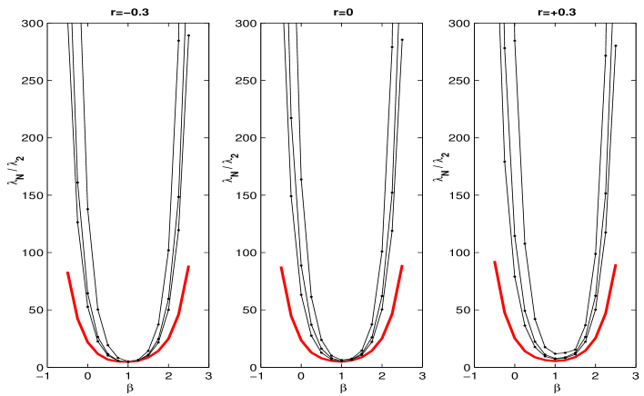
Figure 6: Plots of $\lambda_{N}/\lambda_{2}$ as varying $\beta$ for scale free networks with different values of the power-law exponent $\gamma=[2.5,3,3.5]$. On the left plot we show negatively correlated networks ($r=-0.3$), on the right positively correlated ones ($r=+0.3$), in the center, networks characterized by absence of degree correlation ($r=0$). The thick lines represent the behavior of the eigenratio for random networks ($\gamma=\infty$). $N=10^{3}$ nodes, $\mathcal{E}=4\cdot 10^{3}$.

In this section we shall extend the results presented above to the case of weighed topologies. Interestingly in [?, ?], it has been shown that an appropriate choice of weights over the network links, may improve considerably the network synchronizability. In [?], it has been shown that such improvement is highest if the weights are set to be proportional to a particular topological property at the network links, termed as load or betweenness centrality.

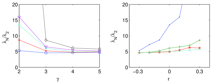
Figure 7: Synchronizability of degree correlated networks in the optimal regime ($\beta=1$). Left figure: behavior of the eigenratio $\lambda_{N}/\lambda_{2}$, as a function of $\gamma$. $N=10^{3}$, $\mathcal{E}=4\cdot 10^{3}$. Legend is as follows: $r=-0.3(o)$, $r=-0.1(\times)$, $r=0(*)$, $r=0.1(\triangledown)$, $r=0.3(\diamondsuit)$. Right side: behavior of the eigenratio $\lambda_{N}/\lambda_{2}$ as a function of the correlation coefficient $r$, for $\gamma$ varying from 2 to 5. $N=10^{3}$, $\mathcal{E}=4\cdot 10^{3}$. Legend is as follows: $\gamma=2(\cdot)$ , $\gamma=3(+)$, $\gamma=4(*)$, $\gamma=5(\times)$.

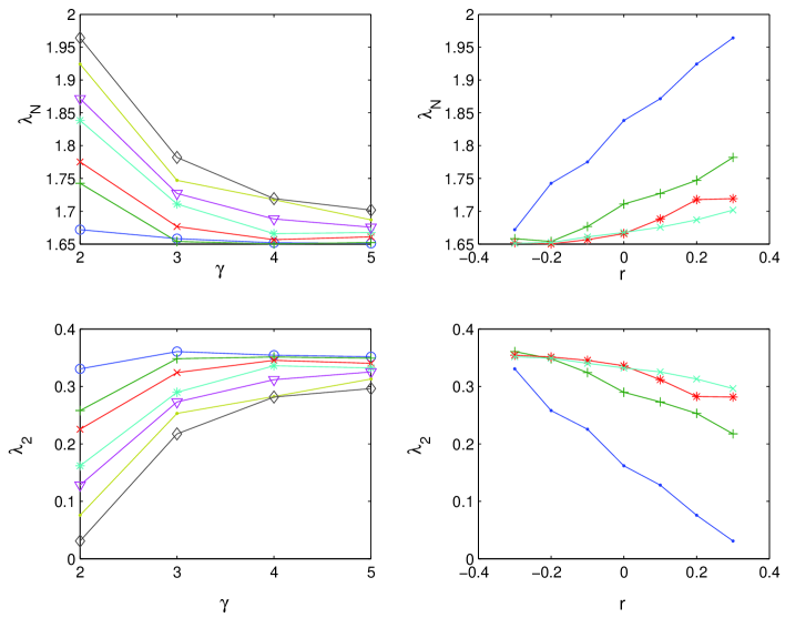
Figure 8: Synchronizability of degree correlated networks in the optimal regime ($\beta=1$). $N=10^{3}$ nodes, $\mathcal{E}=4\cdot 10^{3}$. Behavior of the highest eigenvalue $\lambda_{N}$ (a) and of the second lowest one $\lambda_{2}$ (c), as functions of the correlation coefficient $r$, for $\gamma=[2,3,4,5]$. Behavior of the highest eigenvalue $\lambda_{N}$ (b) and of the second lowest one $\lambda_{2}$ (d), as functions of $\gamma$, for $r=[-0.3,0,+0.3]$. Legend in (a) and (c) is as follows: left side, $r=-0.3(\circ)$, $r=-0.2(+)$, $r=-0.1(\times)$, $r=0(*)$, $r=0.1(\triangledown)$, $r=0.2(\cdot)$, $r=0.3(\diamondsuit)$. Legend in (b) and (d) is as follows: $\gamma=2(\cdot)$ , $\gamma=3(+)$, $\gamma=4(*)$, $\gamma=5(\times)$.

We have seen sofar that scale-free networks can synchronize better as the degree distribution exponent $\gamma$ is increased and the degree correlation coefficient $r$ is decreased. In [?], it was shown that synchronizability of such networks can be further enhanced by an appropriate choice of the network coupling weights, that takes into account exclusively topological information. Specifically, it was found that in order to enhance the synchronizability of heterogeneous networks, the coupling matrix should have the form:

$$\mathcal{L}=D^{-\beta}(D-A),$$ (17)

where the strength of the coupling, for each edge, is scaled by a power (with exponent $\beta$) of the degree of the starting node. Note that, by tuning the parameter $\beta$, it is possible to vary the strength of the coupling from high to low degree vertices and viceversa. Also, from (17), $\mathcal{L}$ can be rewritten as $D^{-\beta/2}(D-A)D^{-\beta/2}$ and thus, even if $\mathcal{L}$ is not symmetric, its spectrum is always real, whatever the value of $\beta$.

In [?], in the case of heterogeneous networks, an optimal coupling was found to be $\beta=1$ in (17). It is worth noting that this leads to asymmetric coupling. Take for example the link between an high degree and a low degree vertex; a coupling of the form (17), with $\beta=1$, results in the low degree node having a much higher influence on the higher degree one than viceversa.

Generally speaking, the case of $\beta=1$, with the weights of the incoming links at each vertex summing to -1 (so that $\mathcal{L}_{ii}=1\quad\forall i$), is of particular interest in that all the networks satisfying this constraint, become directly comparable among themselves, in terms of their spectral properties [?] (see also [?].) In fact, according to the Gerschgorin’s circle theorem, all the eigenvalues ($\lambda_{j}=\lambda_{j}^{r}+j\lambda_{j}^{i},\quad j=1,2,...,N$) of these network are known to belong to a bounded region of the complex plane, and specifically the circle of radius 1, centered at 1 on the real axis [?]. Thus all the $\lambda_{j}^{r}$, are constrained to belong to the interval [0,2] (i.e. $0=\lambda_{1}^{r}\leq\lambda_{2}^{r}\leq...\leq\lambda_{N}^{r}\leq 2$) and the $\lambda_{j}^{i}$ to the interval [-1,1], $j=1,2,...,N$ (in the case of interest here of eq. (17), $\lambda_{j}^{i}=0\quad\forall j$). Moreover the case of $\beta=1$ has been shown to represent an optimum in terms of the network synchronizability, independently from the form of its degree distribution.

Moreover in [?], it was claimed that in the optimally coupled network ($\beta=1$), synchronizability is solely determined by the average degree, while heterogeneity in the network connectivity does not affect synchronization. However, as shown in Sec. 4.1, we observe that in the case of assortative mixing, this is not true anymore; specifically in the particular case of $r=0.3$ shown in the right panel of Fig. 6, homogenous networks are found to behave better than heterogenous ones, even in the optimal case of $\beta=1$.

4.1 Effects of degree correlation

Here, we will show that, assuming a coupling of the form (17), the presence of degree correlation does not alter the optimal value for $\beta$ and better synchronizability properties are still detected when $\beta=1$ as was observed in the uncorrelated case. Moreover, the presence of degree correlation, unlike heterogeneity, does continue to have an effect on the network synchronizability, even in the optimal regime. (Namely, as in the case of unweighed coupling, disassortative mixing always enhances network synchronization).

In Fig. 6 we have reported the behavior of the eigenratio as varying $\beta$ in networks with different degree correlation properties (characterized by $r=[-0.3,0,+0.3]$). Our numerics confirm that the eigenratio $R=\lambda_{N}/\lambda_{2}$ is characterized by a peaked minimum at $\beta\simeq 1$, independently from the value of $r$ (i.e. also when $r\neq 0$). Note that in the case of uncorrelated networks, when $\beta=1$, the eigenratio is quite insensible to the specific form of the degree distribution, as claimed i.e. in [?]. Nonetheless, as $r$ increases, the eigenratio appears to be more sensible to variations in the degree distributions, even in the optimal case of $\beta=1$. Specifically, as shown in Fig. 7, in such a case the minimum is more pronounced for higher values of $\gamma$ (i.e. the paradox of heterogeneity is still present even at $\beta=1$).

Differently from the case of unweighed networks, we notice that in Fig. 8 $~{}\lambda_{N}$ is now sensible to variations in $r$, when compared to $\lambda_{2}$; thus the behavior of the eigenratio $R$ as $r$ varies, cannot be explained only in terms of the second smallest eigenvalue but is a combination of variations of both the eigenvalues (see Fig. 8(a) and 8(c)). The behavior of $\lambda_{2}$ and $\lambda_{N}$ under variations of $\gamma$ for different values of $r$ is shown in Fig. 8(b)-(d). Namely, when increasing $\gamma$, we observe a rise in $\lambda_{2}$ and at the same time, a decrease in $\lambda_{N}$, leading to an overall decrease of the eigenratio $R$ and therefore better synchronizability. Similarly, when $r$ is varied from the disassortative ($r<0$) to the assortative ($r>0$) regime, we observe both a decrease in $\lambda_{2}$ and an increase in $\lambda_{N}$, leading to a rise in the eigenratio $R$.

Observe that in the case of the normalized Laplacian (17) considered here, the following relationship from graph theory is valid [?]:

$$\frac{{h^{\prime\prime}}_{G}^{2}}{2}<\lambda_{2}\leq 2{h^{\prime\prime}}_{G},$$ (18)

where $h^{\prime\prime}_{G}=\min_{S}h^{\prime\prime}_{G}(S)$ and $h^{\prime\prime}_{G}(S)$ is defined as:

$$h^{\prime\prime}_{G}(S)=\frac{{\mathcal{D}(S)}}{\min{(vol(S),vol(\bar{S})})},$$ (19)

with $vol(S)=\sum_{i\in S}k_{i}$. Note that in this case $h^{\prime\prime}_{G}(S)$ can be estimated as:

$${h^{\prime\prime}}_{G}({\mathbf{y}},r)=\frac{{(\mathbf{y}}^{T}{\mathbf{q}}-{\mathbf{y}}^{T}E{\mathbf{y}})}{\min({\mathbf{y}}^{T}{\mathbf{q}},\quad(\bf{1}-{\mathbf{y}}^{T}){\mathbf{q}})}.$$ (20)

Then it is sufficient to observe that, for each $S$, the denominator in (20) is a quantity independent from $r$, and it becomes straightforward to obtain the existence of an upper and a lower bound for $\lambda_{2}$, decreasing with $r$. Unfortunately notwithstanding this, estimating the effects of $r$ on $\lambda_{N}$ resulted to be a non-trivial task and therefore it remains an open problem. An important feature seems to be the symmetry between the behavior of $\lambda_{2}$ and $\lambda_{N}$ reported in Fig.  8(a)-(c) and  8(b)-(d).

From the numerics shown in Fig. 8, we observe a clear advantage of introducing negative degree correlation within the network (in terms of both $\lambda_{N}$ and $\lambda_{2}$), when $\beta=1$. Thus we expect to observe an enlargement of the synchronization interval $I_{\sigma}$, for both higher and lower values of $\sigma$ as decreasing $r$. Moreover, since this happens for whatever a choice of $\beta$, we find that disassortative mixing always enhances synchronization.

The effects of correlation on the eigenratio $R$ in the case of $\beta=1$ (i.e. optimal synchronizability) is fully illustrated in Figs. 7 and 8. Specifically from Figs. 7 and 8, we observe that negatively correlated networks continue to show higher synchronizability, for every value of the exponent $\gamma$. This indicates that the effects of correlation on $R$ are not dampened by the presence of an appropriate coupling of the form (17). Fig. 7 also shows a non-negligible dependence of the eigenratio on the exponent of the power-law distribution $\gamma$, indicating that heterogeneity continues to affect the synchronizability of weighed correlated networks, especially in the cases where $r>0$ (as also shown in the right panel of Fig. 6).

5 Effects of degree correlation on the synchronization dynamics

Now, we shall seek to investigate the effects of variable degree correlation on the dynamics of networks of oscillators. Specifically in what follows we will evaluate the behavior of dynamical networks of (i) identical and (ii) non identical oscillators.

As an example of identical oscillators, we consider a network of coupled chaotic Rössler oscillators, connected as in (1). In [?], we have already reported numerical results showing the synchronization dynamics of such networks in the case where $h(x)=Ix$, with $I$ being the 3-dimensional identity matrix. Therein we observed that negative degree correlation does indeed have beneficial effects on the network synchronization. Specifically, our preliminary results confirmed that negative degree correlation is able to enhance the network synchronization dynamics.

Here we suppose the dynamics at each node $i$ to be described by the following vector field, ${\bf{v_{i}}}=(x_{i},y_{i},z_{i})$:

$$\dot{x}_{i}= -y_{i}\;-\;z_{i}-\sigma\sum_{j=1}^{N}{\mathcal{L}_{ij}}x_{j}$$

$$\dot{y}_{i}= x_{i}\;+\;0.165y_{i}$$

$$\dot{z}_{i}= 0.2+(x_{i}-10)z_{i}-\sigma\sum_{j=1}^{N}{\mathcal{L}_{ij}}z_{j}$$

where $\sigma$ is the tunable strength of the coupling. Note that, according to this scheme, we have chosen the Rössler to be coupled through the variables $x$ and $z$. The reason is that under this assumptions, the MSF results to be negative in a bounded range of values of the parameter $\alpha$, yielding that the coupling $\sigma$ should be neither too low, nor too high.

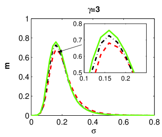
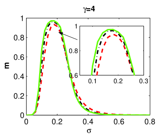
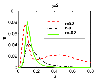
Figure 9: Synchronization dynamics over unweighed networks ($\beta=0$). The plots show the order parameter at regime $m$ for networks characterized by different $\gamma$ (in each subplot) and $r$ (differently colored lines) for increasing values of the coupling gain $\sigma$; $N=10^{3}$, $\mathcal{E}=4\cdot 10^{3}$. Note the different scale on the y-axis in the lower figure.

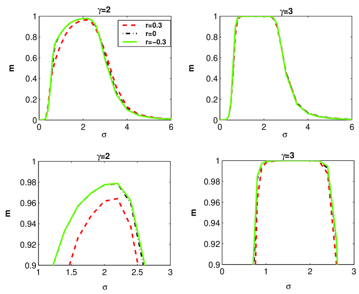
Figure 10: Synchronization dynamics over weighed networks ($\beta=1$). The plots show the order parameter at regime $m$ for networks characterized by different $\gamma$ (in each subplot) and $r$ (differently colored lines) for increasing values of the coupling gain $\sigma$; $N=10^{3}$, $\mathcal{E}=4\cdot 10^{3}$. The lower plots are enlargements of the upper ones. In the right-low panel, it is interesting to observe how the range of values of $\sigma$ for which synchronization is achieved (at $m=1$) increases as $r$ is reduced from 0.3 to -0.3.

We have performed simulations over scale-free complex networks, with variable power-law exponents, characterized by several values of the degree correlation coefficient (typically in the range $r\in[-0.3,+0.3]$).

In order to have a measure of the overall network synchronization, we introduce the order parameter $m(t)\in[0,1]$, defined as follows (see also [?]):

$$m(t)={1\over N(N-1)}\sum_{j\neq i,i,j=1}^{N}\Theta(\delta-d_{ij}(t)),$$ (21)

where $\Theta(x)$ is the Heavyside function, i.e. $\Theta(x)=1$ if $x\geq 0$ and $\Theta(x)=0$ otherwise. The parameter $\delta$ is a small number to account for the finite numerical accuracy, (here we have chosen $\delta=10^{-2}$), so that two states in phase space lying inside a sphere of radius $\delta$ are considered as mutually being synchronized. The parameter $m(t)$ gives the fraction of pairs of elements $(i,j)$ which are synchronized at time $t$ (i.e., $d_{ij}\leq\delta$). This fraction is equal to unity if all possible pairs are synchronized and zero if no pair is synchronized, with intermediate values $0<r<1$ indicating partial synchronization. In what follows we will look at the asymptotic average value of $m(t)$, say $m$, as function of the coupling strength $\sigma$.

Specifically, in Figs. 9 and 10, a double phase transition is observed: the first one from a non-synchronous to a synchronous regime as the coupling strength is increased; the second one from the synchronous to a non-synchronous phase as the coupling strength is further increased and exceeds a critical value.

At first, we suppose the network topology to be unweighed, i.e. the coupling is identical over all the edges and equal to 1. In order to explore the effects of the network structure (degree distribution and degree correlation) on the dynamical synchronization process, we have performed several numerical simulations, the main results being illustrated in Fig. 9. The asymptotic value of the order parameter $m$, has been computed for networks with different topological features. We have compared scale free networks characterized by different power-law exponents and we found that, as can be observed by comparing the plots in Fig. 9, homogenous networks (characterized by higher values of $\gamma$) synchronize better than heterogenous ones (note the different scale on the y-axis in the lower plot, where heterogeneous scale-free networks, with $\gamma=2$ cannot be synchronized in practice for any value of $\sigma$). This indicates that an high heterogeneity in the degree distribution can result in being very harmful to the overall synchronization [?]. Moreover negative degree correlation is seen to enhance the network synchronizability, for all the values of $\gamma$ considered (excluding those for which synchronization cannot be achieved, e.g. $\gamma=2$ in Fig. 9, where $m\ll 1$). This is consistent with the predictions based on the eigenvalue analysis provided in Sec. 3 and confirms the beneficial role played by negative degree correlation with respect to networks synchronization even in terms of synchronization dynamics.

The case of weighed topologies, (i.e. when $\beta=1$) is shown in Fig. 10. Again, negative degree correlation is observed to enhance the network synchronization, at high values of the order parameter when $m\approx 1$. Moreover, as shown in Fig. 10, the network synchronization is reduced as the heterogeneity in the degree distribution is increased (i.e for lower values of the exponent $\gamma$). This indicates that, even in the optimal regime where $\beta=1$, networks characterized by variable degree distributions, behave differently in terms of their synchronization dynamics (practically we observe an analogous phenomenon as in the case of the unweighed topologies). Also, it is interesting to observe in Fig. 10 that the range $I_{\sigma}$ of values of $\sigma$ for which synchronization is completely achieved (at $m=1$), increases by reducing $r$ from 0.3 to -0.3.

It is worth noting here that, by comparing Figs. 9 and 10, weighed networks, in which the strength of the coupling has been rescaled by the degree at each node, are more synchronizable than unweighed ones (as also predicted by the behavior of the eigenratio in Fig. 6). We wish to emphasize that all the numerical results provided in this section, are in good agreement with the eigenvalue analysis presented in Sec.3.

6 Conclusions

The structure of many real world networks is characterized by non-trivial degree-degree correlation in the network connections. This leads alternatively to disassortative mixing in biological and technological networks and assortative mixing in social networks. In this paper we have studied the effect of degree correlation on the network synchronizability and synchronization dynamics. Specifically, we studied the effects of correlation on the Laplacian eigenratio, a parameter proposed in [?] as a measure of the synchronizability of a network of coupled nonlinear oscillators.

We have found that disassortative mixing, which is typical of biological and technological networks, plays a positive role in enhancing network synchronizability. The numerical observations were confirmed by the analytical estimates found for the Laplacian eigenratio, which were shown to be well suited to describe the observed phenomena.

Following [?], we then analyzed the effects of weighted and directed coupling of the form (17) and found that the presence of correlation continues to affect synchronization with disassortative weighted networks synchronizing better than assortative ones. We noticed that, even in the presence of degree correlation, synchronizability seems to be optimal when the strength of the coupling along each edge is made inversely proportional to the degree of the starting node. Though a common belief is that when such coupling is considered, heterogeneity becomes unable to suppress synchronization, our numerics show that an exception to this paradigm is represented by the case of assortatively mixed networks, where the effect of the degree distribution is found to be strongly enhanced.

Using a nonlinear optimization approach we found that negative degree correlation is naturally attained by the network when the aim is to minimize $\lambda_{2}$ and hence enhance synchronizability. Thus, we conjectured that disassortative mixing has played the role of a self organizing principle in leading the formation of many real world networks as the Internet, the World Wide Web, proteins interactions, neural and metabolic networks.

Finally, we investigated the synchronization dynamics of both weighed and unweighed networks of identical Rössler oscillators, confirming the theoretical results obtained in the paper. A more general case of weighed degree correlated networks (with complex spectrum of the Laplacian) will be discussed elsewhere [?].

References

- [1]
- [2] [] A.L.Barabasi & R.Albert [1999], ‘Emergence of scaling in random networks’, Science 286, 509–512.
- [3]
- [4] [] Amaral, L., Scala, A., M.Berth lemy & H.E.Stanley [2000], ‘Classes of small-world networks’, Proc.Natl.Acad.Sci.USA 97, 11149–11152.
- [5]
- [6] [] Arrowsmith, D., di Bernardo, M. & F.Sorrentino [2005], ‘Effects of variation of load distribution on network performance’, Proc. IEEE ISCAS, Kobe, Japan pp. 3773–3776.
- [7]
- [8] [] A.T.Winfree [1980], The geometry of biological time, Springer, New York.
- [9]
- [10] [] A.Vasquez, R.Pastor-Satorras & A.Vespignani [2002], ‘Large-scale topological and dynamical properties of the internet’, Phys.Rev.E. 65, 066130.
- [11]
- [12] [] B.Mohar [1989a], ‘Isoperimetric number of graphs’, J. Comb. Theory B(47), 274–291.
- [13]
- [14] [] B.Mohar [1989b], ‘The laplacian spectrum of graphs’, Graph Theory, Combinatorics, and Applications 2, 871–898.
- [15]
- [16] [] Boccaletti, S., V.Latora, Y.Moreno, M.Chavez & D.U.Hwang [2006], ‘Complex networks: Structure and dynamics’, Physics Reports 424(4-5), 175–308.
- [17]
- [18] [] Catanzaro, M., Boguna, M., & Pastor-Satorras, R. [2005], ‘Generation of uncorrelated random scale-free networks’, Phys. Rev. E 71(2), 027103.1–027103.4.
- [19]
- [20] [] Chavez, M., D.U.Huang, Amann, A., Hentschel, H. & S.Boccaletti [2005], ‘Synchronization is enhanced in weighted complex networks’, Phys. Rev. Lett. 94, 218701.
- [21]
- [22] [] Chung, F. [1997], Spectral Graph Theory, American Mathematical Society.
- [23]
- [24] [] di Bernardo, M., Garofalo, F. & Sorrentino, F. [2006], ‘Effects of degree correlation on the synchronization of networks of oscillators.’, Accepted for publication on International Journal of Bifurcation and Chaos.
- [25]
- [26] [] D.J.Watts & S.H.Strogatz [1998], ‘Collective dynamics of ’small world’ networks’, Nature 393, 440–442.
- [27]
- [28] [] D.S.Callaway, J.E.Hopcroft, J.M.Kleinberg, Newman, M. & S.H.Strogatz [2001], ‘Are randomly grown graphs really random?’, Physical Review E 64, 0419021.1–0419021.7.
- [29]
- [30] [] D.U.Huang, Chavez, M., Amann, A. & S.Boccaletti [2005], ‘Synchronization in complex networks with age ordering’, Phys. Rev. Lett. 94, 138701.
- [31]
- [32] [] Erdos, P. & A.Renyi [1960], ‘On the evolution of random graphs’, Publ. Math. Inst. Hung. Acad. Sci. A 5, 17–61.
- [33]
- [34] [] Fan, J. & Wang, X. F. [2005], ‘On synchronization in scale free dynamical networks’, Physica A 349, 443–451.
- [35]
- [36] [] G.B.Ermentrout & N.Kopell [1984], ‘Frequency plateaus in a chain of weakly coupled oscillators’, SIAM J. Math. Analysis (15), 215–237.
- [37]
- [38] [] Goh, K.-I., Kahng, B. & D.Kim [2001], ‘Universal behavior of load distribution in scale-free networks’, Phys.Rev.Lett. 87, 278701.
- [39]
- [40] [] J.Cheeger [1970], ‘A lower bound for the smallest eigenvalue of the laplacian’, Problems Anal. pp. 195–199.
- [41]
- [42] [] J.Park & M.E.J.Newman [2003], ‘The origin of degree correlations in the internet and other networks’, Phys.Rev.E 68, 026112.
- [43]
- [44] [] Lee, D.-S. [2005], ‘Synchronization transition in scale-free networks: Clusters of synchrony’, Phys.Rev.E 72, 026208.
- [45]
- [46] [] Lee, J., Goh, K.-I., Kahng, B. & Kim, D. [2006], ‘Intrinsic degree-correlations in the static model of scale-free networks’, Euro. Phys. J. B 49, 231–238.
- [47]
- [48] [] L.M.Pecora & T.L.Carroll [1998], ‘Master stability functions for synchronized coupled systems’, Phys.Rev.Lett. 80, 2109–2112.
- [49]
- [50] [] Lu, J., Chen, G. & Cheng, D. [2004], ‘Characterizing the synchronizability of small-world dynamical networks’, IEEE Transactions on Circuits and Systems 51(4), 787–795.
- [51]
- [52] [] M.Barahona & L.M.Pecora [2002], ‘Synchronization in small-world networks’, Phys.Rev.Lett. 89, 054101.
- [53]
- [54] [] M.Berth lemy [2004], ‘Betweenness centrality in large complex networks’, Eur. Phys. Jour. B 38, 163.
- [55]
- [56] [] Mirollo, R. & S.H.Strogatz [1990], ‘Synchronization of pulse-coupled biological oscillators’, SIAM J. Appl. Math. 50, 1645–1662.
- [57]
- [58] [] M.Molloy & B.Reed [1995], ‘A critical point for random graphs with a given degree sequence’, Random Structures and Algorithms (6), 161–179.
- [59]
- [60] [] Motter, A., Zhou, C. & J.Kurths [2005a], ‘Enhancing complex-network synchronization’, Europhys. Lett.
- [61]
- [62] [] Motter, A., Zhou, C. & J.Kurths [2005b], ‘Network synchronization, diffusion, and the paradox of heterogeneity’, Phys.Rev.E 71, 016116.
- [63]
- [64] [] N.Alon [1986], ‘Eigenvalues and expanders’, Combinatorica 6(2), 83–96.
- [65]
- [66] [] Newman, M. [2002a], ‘Assortative mixing in networks’, Phys. Rev. Lett. 89, 208701.
- [67]
- [68] [] Newman, M. [2002b], ‘The spread of epidemic disease on networks’, Phys. Rev. E 66, 016128.
- [69]
- [70] [] Newman, M. [2003], ‘Mixing patterns in networks’, Phys. Rev. E 67, 026126.
- [71]
- [72] [] N.Kopell & G.B.Ermentrout [1986], ‘Simmetry and phaselocking in chains of weakly coupled oscillators’, Commun. Pure Appl. Math. (39), 623–660.
- [73]
- [74] [] Oh, E., Rho, K., Hong, H. & B.Kahng [2005], ‘Modular synchronization of complex networks’, Phys.Rev.E 72, 047101.
- [75]
- [76] [] R.Pastor-Satorras & A.Vespignani [2001], ‘Epidemic spreading in scale-free networks’, Phys. Rev. Lett. 86(14), 3200 3203.
- [77]
- [78] [] S.H.Strogatz [2001], ‘Exploring complex networks’, Nature 410, 268–276.
- [79]
- [80] [] S.H.Strogatz & Stewart, I. [1993], ‘Coupled oscillators and biological synchronization’, Scientific American 269(6), 102–109.
- [81]
- [82] [] S.Kirkpatrick, C.D.J.Gerlatt & M.P.Vecchi [1982], ‘Optimization by simulated annealing’, IBM Research Report RC.
- [83]
- [84] [] Sorrentino, F., di Bernardo, M., Cuellar, G. H. & Boccaletti, S. [2006], ‘Synchronization in weighted scale-free networks with degree-degree correlation’, Accepted for publication on Physica D.
- [85]
- [86] [] T.Nishikawa, Motter, A., Y.Lai & F.C.Hoppensteadt [2003], ‘Heterogeneity in oscillator networks: Are smaller worlds easier to synchronize?’, Phys.Rev.Lett. 91, 014101.
- [87]
- [88] [] Wu, C. W. [2003], ‘Perturbation of coupling matrices and its effects on the synchronizability in arrays of coupled chaotic systems’, Physics Letters A 319(5-6), 495–503.
- [89]
- [90] [] X.F.Wang [2002], ‘Complex networks: Topology dynamics and synchronization’, International Journal of Bifurcation and Chaos 12(5), 885–916.
- [91]
- [92] [] Y.Kuramoto [1984], Chemical Oscillations, Waves and Turbolence, Springer, Berlin.
- [93]
- [94] [] Y.Moreno & F.Pacheco, A. [2004], ‘Synchronization of kuramoto oscillators in scale-free network’, Europhys. Lett. 68(4), 603–609.
- [95]
- [96] [] Y.Moreno, Vazquez-Prada, M. & F.Pacheco, A. [2004], ‘Fitness for synchronization of network motifs’, Physica A 343, 279.
- [97]
- [98] [] Yook, S.-H. & Meyer-Ortmanns, H. [2005], ‘Synchronization of rossler oscillators on scale-free topologies’, Physica A 371, 781.
- [99]