Band structures of P-, D-, and G-surfaces

Abstract

We present a theoretical study on the band structures of the electron constrained to move along triply-periodic minimal surfaces. Three well known surfaces connected via Bonnet transformations, namely P-, D-, and G-surfaces, are considered. The six-dimensional algebra of the Bonnet transformations [C. Oguey and J.-F. Sadoc, J. Phys. I France 3, 839 (1993)] is used to prove that the eigenstates for these surfaces are interrelated at a set of special points in the Brillouin zones. The global connectivity of the band structures is, however, different due to the topological differences of the surfaces. A numerical investigation of the band structures as well as a detailed analysis on their symmetry properties is presented. It is shown that the presence of nodal lines are closely related to the symmetry properties. The present study will provide a basis for understanding further the connection between the topology and the band structures.

I Introduction

For nearly two decades intense efforts have been devoted to the studies of periodic curved surfaces as topological objects to describe certain structured materials. Several conceptually different classes, such as zero-potential surfaces, nodal surfaces, and periodic minimal surfaces, often share similar properties concerning topology and symmetry.SN91 ; AHLL88 Such a surface can be constructed as a space partitioner which is invariant under space group operations, hence the space group symmetries are the key ingredients of them. In reality, on the other hand, such surfaces are realized as nanometer to micron scale interface structures in lyotropic liquid crystals or cell membranes. Furthermore, recent progress in the synthesis of nano-structured materials prompts us to consider the possibility of using these materials as the templates for electronic devices embracing interesting geometrical properties.

The present paper deals with a fundamental problem on the electronic structures of materials characterized by periodic curved surfaces. The theoretical basis of the quantum mechanics of electrons confined within thin curved films has been developed by several authors.JK71 ; C81 ; C82 ; IN91 ; DE95 ; CEK04 They showed that when the electron is strongly constrained onto a smoothly curved surface, the quantization of the motion perpendicular to the surface results in an effective potential energy depending on the local curvatures along the surface. Since this potential energy is attractive, the electron can be weakly bounded around a curved region of the surface (geometrically induced bound states). Theoretical interests also arise in regard to quantum chaos, since the constrained motion on a surface with non-zero intrinsic curvatures entails classical chaos.BV86 These studies, however, deal primarily with the local effects of curvatures. The roles played by the symmetry and topology of the surface on the determination of electronic structures have largely remained intact, apart from that Aoki et al. numerically studied the band structures of triply periodic minimal surfaces recently.AKTMK01 ; KA05 The aim of the present paper is to perform a more thorough investigation into the electronic structures of similar periodic curved surfaces.

In Sec.II, we provide a mathematical background for periodic minimal surfaces and introduce the three basic surfaces in the same Bonnet family, i.e., P-, D-, and G-surfaces, which will be studied further. In Sec.III, the translational subgroups of these three surfaces are described as orthogonal projections of an identical six-dimensional (6D) translational subgroup onto 3D subspaces. A numerical investigation of the band structures of the three surfaces is presented in Sec.IV following a brief summary of the basic formulation of the one-electron problem constrained onto a surface embedded in 3D space. In Sec.V the algebraic information given in Sec.III is used to prove certain interrelations between the band structures of the three surfaces. More precisely, we propose the idea of “band intersections” to show that the energy eigenvalues at a certain set of wave vectors coincide among the three surfaces. In Sec.VI the symmetry properties of energy bands, i.e., the corresponding irreducible representations (IR’s) of the space groups, are analyzed. Based on the IR’s, several features of the band structures and eigenstates are discussed, including the band sticking phenomena and the occurrence of nodal lines. In particular, a general connection is established between the symmetry properties (or IR’s) of the eigenstates and the types of nodal lines entailed by symmetry. The exhaustive lists of IR’s with such nodal lines are shown. Further discussions are given in the last section.

II Periodic minimal surfaces

Curved surfaces are naturally realized as interfaces, and their formation is dominated by surface energies (e.g. surface tension). Like soap films on closed wire frames, they often resemble minimal surfaces, that is, surfaces with vanishing mean-curvature. Minimal surfaces are privileged mathematically since they have an analytic representation called the Weierstrass-Enneper (WE) representation:S75 ; O86 a minimal surface is represented by the real part of a complex vector ${\bf z}$ in a 3D complex space ${\bf C}^{3}\,(\simeq E_{6})$ multiplied by a phase factor:

$${\bf r}(w)={\rm Re}\left(e^{i\alpha}{\bf z}(w)\right),$$ (1)

$${\bf z}(w)=\ell\left(\int^{w}\!\!F(\zeta)(1-\zeta^{2}){\rm d}\zeta,\,\int^{w}\!\!iF(\zeta)(1+\zeta^{2}){\rm d}\zeta,\,\int^{w}\!\!2F(\zeta)\zeta{\rm d}\zeta\right),$$ (2)

where $\ell$ is an overall scale factor, $\alpha$ the Bonnet angle, $w=q^{1}+iq^{2}$, and $F(\zeta)$ a complex analytic (or holomorphic) function associated with the Bonnet family of minimal surfaces.BonnetFamily Hence the surface is represented as a multiple-valued function of the complex variable $w$, where different integration paths give distinct points on the surface. The two real variables, $q^{1}$ and $q^{2}$, serve as the isothermal parameterization of the surface.

Minimal surfaces with periodicity in three independent directions are called triply periodic minimal surfaces (TPMS’s). The importance of TPMS’s as topological objects describing interface materials like self-assembled lyotropic liquid crystals has been recognized for nearly two decades.AHLL88 ; CS87 ; SC89 Compared to other classes of periodic surfaces like zero-potential surfaces,SN91 TPMS’s are especially advantageous for physical applications because Eq.(1) provides a parameterization of the surface for incorporating it into written equations. In the following, we focus on the classical examples of Schwarz’s P- and D-surfacesSchwarz and Sch$\ddot{\rm o}$n’s G-surface (gyroid)Schoen which belong to the cubic system. The corresponding WE function, $F(\zeta)$, is given by

$$F(\zeta) = \frac{1}{\sqrt{1+14\zeta^{4}+\zeta^{8}}},$$ (3)

with eight branch points of order 2 at $\zeta=(\sqrt{3}\pm 1)/\sqrt{2}e^{2\pi in/4}$ ($n=0,1,2,3$) on its Riemann surface.RiemannSurface For each of the three surfaces, the Bonnet angle $\alpha$, has to take a proper value as will be given below. Multiple surfaces in the same Bonnet family are intrinsically identical, or isometric, apart from the global topology. The surfaces are obtained from one another via Bonnet transformation, namely the change of $\alpha$.

We may write ${\bf z}(w)={\bf u}(w)+i{\bf v}(w)$ with ${\bf u}(w)$ and ${\bf v}(w)$ being two real vectors, hence ${\bf r}(w)={\bf u}(w)\cos{\alpha}-{\bf v}(w)\sin{\alpha}$. Alternatively, one may introduce a 6D vector, $\Xi(w)=({\bf u}(w),\,{\bf v}(w))$, and the minimal surface ${\bf r}(w)$ is given as the orthogonal projection of $\Xi(w)$ onto a 3D subspace specified by the hyper-rotation angle $\alpha$. P- and D-surfaces are given by the Bonnet angles, $\alpha_{P}=0$ and $\alpha_{D}=90^{\circ}$, hence they are given by ${\bf u}(w)$ and $-{\bf v}(w)$, respectively. Accordingly the 6D space $E_{6}$ embedding $\Xi(w)$ is divided into two 3D subspaces as $E_{6}=E_{P}\oplus E_{D}$, where $E_{P}$ and $E_{D}$ are the embedding subspaces for P- and D-surfaces, respectively.

It is convenient to define an orthogonal transformation of $E_{6}$ by the 6D orthogonal matrix

$$O(\alpha):=\left(\begin{array}[]{cr}{\bf I}\cos\alpha&-{\bf I}\sin\alpha\\ {\bf I}\sin\alpha&{\bf I}\cos\alpha\end{array}\right)$$ (6)

with ${\bf I}$ being the 3D identity matrix; the two 3D subspaces, $E_{P}$ and $E_{D}$, are mixed by such a transformation. Then Eq.(1) can be written concisely as ${\bf r}(w)=\Pi_{P}O(\alpha)\Xi(w)$, where $\Pi_{P}$ is the orthogonal projector onto $E_{P}$ defined by $({\bf I}~{}~{}{\bf O})$ with ${\bf O}$ being the 3D zero matrix. G-surface is obtained by choosing the Bonnet angle as $\alpha_{G}=\arctan{(r/s)}\approx 51.985^{\circ}$. Here the constants $r$ and $s$ are defined by $r-is=2e^{-\pi i/6}K(k^{2})$, in which $K(k^{2})$ stands for the complete elliptic integral of the first kind and $k=e^{-\pi i/3}$. Their numerical values are $r\approx 2.156$ and $s\approx 1.686$. Hence, G-surface is just the orthogonal projection of $\Xi(w)$ onto a 3D subspace $E_{G}$ which is inclined in the 6D space by the hyper-rotation angle $\alpha_{G}$. The relevant orthogonal projector is given by $\Pi_{G}=\Pi_{P}O(\alpha_{G})$. One may also find that the orthogonal projector for D-surface is given by $\Pi_{D}=\Pi_{P}O(\alpha_{D})=-({\bf O}~{}~{}{\bf I})$.

III Crystallography of Bonnet transformations

With each of the three TPMS’s a pair of space groups, $G/H$, is associated; $G$ includes the symmetry elements to reverse the sides of the surface, while $H$ does not. The group $H$ is a subgroup of $G$. The pairs for P-, D-, and G-surfaces are $Im\bar{3}m/Pm\bar{3}m$, $Pn\bar{3}m/Fd\bar{3}m$, and $Ia\bar{3}d/I4_{1}32$, respectively. It is important to note that the Bravais lattices for P- and D-surfaces depend on whether or not to identify the sides of the surfaces. The electronic Hamiltonians for the three TPMS’s to be studied have the symmetry of the group $G$.

The WE formulae for the three surfaces reveal that the fundamental patches of the surfaces, corresponding to the asymmetric unit of the relevant space groups $G$, consist of (2,4,6) triangles.GCMK00 ; (pqr)Triangle More precisely, the fundamental patch of P-surface as well as that of D-surface coincides with a (2,4,6) triangle. That of G-surface, on the other hand, consists of two triangles and is twice as large as those of the other two (c.f. Fig.1). The two triangles for the case of G-surface are not congruent with each other in the embedding space, so that one of them cannot be reproduced via any space group operation from the other. However, they are congruent intrinsically, which implies that G-surface has an additional “intrinsic symmetry” which cannot be reproduced by the space group. The surfaces are thus tessellated into (2,4,6) triangles.

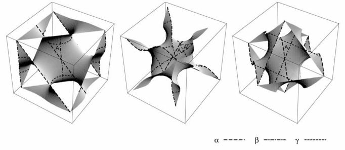
Figure 1: The unit cells of the three TPMS’s obtained by projecting the 6D unit cell (corresponding to the dodecagonal region of the hyperbolic plane) onto the relevant 3D subspaces $E_{P}$, $E_{D}$, and $E_{G}$. Bounding boxes are shown to indicate the relative orientation to the cubic unit cell. The fundamental patch consists of either a single triangle denoted as A (for P- and D-surfaces) or two triangles denoted as A and A^′ (for G-surface). Representative high-symmetry geodesics of type $\alpha$, $\beta$, and $\gamma$ are also indicated on the surfaces. For P-surface these correspond to the two-fold axis $U^{\bar{y}z}$ ($\alpha$), the mirror planes $\sigma^{xy}$ ($\beta$) and $\sigma^{z}$ ($\gamma$). For D-surface, these are the mirror plane $\sigma^{xy}$ ($\alpha$), the two-fold axes $U^{\bar{z}x}$ ($\beta$) and $U^{y}$ ($\gamma$), respectively. For G-surface, no symmetry element corresponds to these geodesics.

A close relationship between the three TPMS’s and the (2,4,6)-tessellation of the hyperbolic plane, i.e., the non-Euclid plane with a constant Gaussian curvature, was pointed out by Sadoc and Charvolin.SC89 They proved that the translational subgroup of the (2,4,6)-tessellation of the hyperbolic plane, where the unit cell is identified as a dodecagonal region consisting of 96 triangles as shown in Fig.2, derives the translational subgroups of the three TPMS’s. The corresponding Bravais lattices are simple cubic (s.c.), face centered cubic (f.c.c.), and body centered cubic (b.c.c.) for P-, D-, and G-surfaces, respectively. The unit cells of the TPMS’s can be taken as dodecagonal patches embedded in three dimensions, as shown in Fig.1, corresponding to the dodecagonal region of the hyperbolic plane. Note that these unit cells are only the primitive unit cells for the space groups, $H$. If the two sides of a surface are indistinguishable, the space group will be $G$ whose primitive unit cell is reduced by half for P- and D-surfaces, and the Bravais lattices become b.c.c. and s.c., respectively.

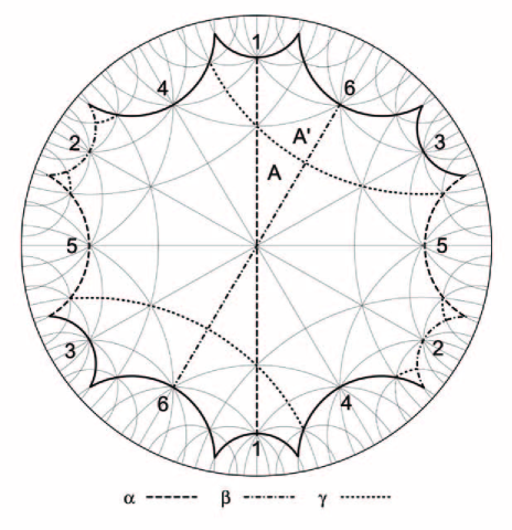
Figure 2: The dodecagonal region of the hyperbolic plane, shown within the Poincar$\acute{\rm e}$ disc, corresponds to the dodecagonal unit patches of P-, D-, and G-surfaces. The identification of the opposite edges yields a genus-3 torus corresponding to the unit cell of $\Xi(w)$ with opposite sides being identified. The tessellation into (2,4,6)-triangles corresponds to the division of the TPMS’s into fundamental patches. There are three types of geodesics passing through high-symmetry points: $\alpha$, passing through six- and four-fold symmetry centers alternately, $\beta$, six- and two-fold centers, and $\gamma$ four- and two-fold centers, respectively. Only a few representatives of each type is indicated. (See also Fig.1.)

The 6D crystallographic description of $\Xi(w)$ was thoroughly investigated by Oguey and Sadoc,OS93 who established that it is a periodic structure. The unit cell of the relevant 6D lattice $\Lambda$ is associated with the aforementioned dodecagonal patch lifted into the 6D space. The primitive lattice vectors of $\Lambda$ are given by the column vectors ofOS93

$${\bf A} = (\vec{t}_{1},\vec{t}_{2},\vec{t}_{3},\vec{\tau}_{1},\vec{\tau}_{2},\vec{\tau}_{3})=\ell\left(\begin{array}[]{cccccc}r&0&0&0&r&-r\\ 0&r&0&-r&0&r\\ 0&0&r&r&-r&0\\ 0&s&-s&0&s&s\\ -s&0&s&s&0&s\\ s&-s&0&s&s&0\\ \end{array}\right).$$ (13)

The translational symmetry of each of the three surfaces is given as the 3D lattice, $\Lambda_{X}$, with $X=P$, $D$, or $G$. Then it is given as $\Lambda_{X}=\Pi_{X}\Lambda$. Specifically, $\Lambda_{P}$ (or $\Lambda_{D}$) is generated by the six column vectors of the upper (or lower) half of ${\bf A}$, so that it is a s.c. (or f.c.c.) lattice with lattice constant $a_{P}:=\ell r$ (or $a_{D}:=2\ell s$). Similarly, $\Lambda_{G}$ is generated by the six column vectors of the matrix

$$\Pi_{G}{\bf A} = \ell\,b\,\left(\begin{array}[]{cccccc}1&-1&1&0&0&-2\\ 1&1&-1&-2&0&0\\ -1&1&1&0&-2&0\\ \end{array}\right)$$ (17)

with $b=rs/\sqrt{r^{2}+s^{2}}$, so that $\Lambda_{G}$ is a b.c.c. lattice with lattice constant $a_{G}:=2\ell b$. In each case, the unit cell is given by the projection of the dodecagonal patch onto the relevant subspace (see Fig.1). The relationship between $\Lambda$ and $\Lambda_{X}$ ($X=P$, $D$, and $G$) is schematically represented in Fig.3.

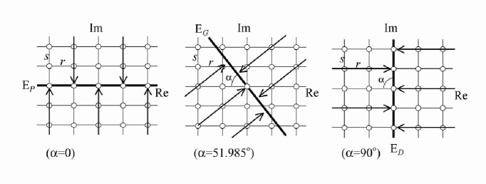
Figure 3: The orthogonal projections of the 6D lattice $\Lambda$ for P- (left), G- (middle), and D-surfaces (right) are shown schematically in the complex plane of each component in ${\bf z}(w)$. The projection map of the lattice points of $\Lambda$ are shown by open circles. The arrows indicate the directions of the orthogonal projections in each plane.

Let us consider the reciprocal lattice $\Lambda^{\ast}$ of $\Lambda$. To do so, we shall take the transposed inverse of A, ${\bf B}=\left({\bf A}^{-1}\right)^{T}$, which is given as

$${\bf B}=\frac{1}{2\ell}\left(\begin{array}[]{cccccc}0&\bar{r}&\bar{r}&0&\bar{r}&-\bar{r}\\ \bar{r}&0&\bar{r}&-\bar{r}&0&\bar{r}\\ \bar{r}&\bar{r}&0&\bar{r}&-\bar{r}&0\\ 0&\bar{s}&-\bar{s}&\bar{s}&0&0\\ -\bar{s}&0&\bar{s}&0&\bar{s}&0\\ \bar{s}&-\bar{s}&0&0&0&\bar{s}\\ \end{array}\right),$$ (24)

with $\bar{r}=1/r$ and $\bar{s}=1/s$. The generators of $\Lambda^{\ast}$ are given as the column vectors of ${\bf B}$. We shall denote these generators as $\vec{Q}_{i}$ ($i=1,...,6$), so that ${\bf B}=(\vec{Q}_{1},\vec{Q}_{2},\vec{Q}_{3},\vec{Q}_{4},\vec{Q}_{5},\vec{Q}_{6})$.

Since the TPMS’s are projections of $\Xi(w)$ onto the 3D subspaces, $E_{P}$, $E_{D}$, and $E_{G}$, their reciprocal lattices, $\Lambda_{P}^{\ast}$, $\Lambda_{D}^{\ast}$, and $\Lambda_{G}^{\ast}$, are the intersections of $\Lambda^{\ast}$ along the relevant 3D subspaces. It can be shown that the sets of the three generators of these reciprocal lattices are given by

$$\begin{array}[]{ll}\left\{~{}\vec{Q_{1}}+\vec{Q_{5}}-\vec{Q_{6}},~{}\vec{Q_{2}}-\vec{Q_{4}}+\vec{Q_{6}},~{}\vec{Q_{3}}+\vec{Q_{4}}-\vec{Q_{5}}~{}\right\}&{\rm for}~{}\Lambda_{P}^{\ast},\\ \left\{~{}-\vec{Q_{2}}+\vec{Q_{3}}+\vec{Q_{4}},~{}\vec{Q_{1}}-\vec{Q_{3}}+\vec{Q_{5}},~{}-\vec{Q_{1}}+\vec{Q_{2}}+\vec{Q_{6}}~{}\right\}&{\rm for}~{}\Lambda_{D}^{\ast},\\ \left\{~{}\vec{Q_{1}}-\vec{Q_{4}}-\vec{Q_{6}},~{}\vec{Q_{2}}-\vec{Q_{4}}-\vec{Q_{5}},~{}\vec{Q_{3}}-\vec{Q_{5}}-\vec{Q_{6}}~{}\right\}&{\rm for}~{}\Lambda_{G}^{\ast}.\end{array}$$ (28)

IV Electronic band structures of the TPMS’s

For clarity, we shall focus on a specific situation in which the electron is constrained to move along the surface, which means that the electron cannot propagate through the region outside the surface. In order to realize the situation, an infinite potential well is introduced to confine the electron within a thin layer of constant thickness $d$ built over the surface. Then by taking the limit of $d\to 0^{+}$, one obtains the Schr$\ddot{\rm o}$dinger equation for the particle constrained to move along the surface.JK71 ; C81 ; C82 ; IN91 Let us assume a curvilinear coordinates $(q^{1},q^{2})$ on the surface, for which the metric tensor $g_{ij}$ ($i,j=1,2$) is defined by ${\rm d}s^{2}=\sum_{ij}g_{ij}{\rm d}q^{i}{\rm d}q^{j}$ where ${\rm d}s$ is an infinitesimal distance. The principal curvatures are denoted as $\kappa_{1}=1/R_{1}$ and $\kappa_{2}=1/R_{2}$, with $R_{1}$ and $R_{2}$ being the radii of curvature. The Schr$\ddot{\rm o}$dinger equation is written as,

$$-\frac{\hbar^{2}}{2m}\frac{1}{\sqrt{g}}\sum_{i,j=1}^{2}\frac{\partial}{\partial q^{i}}\sqrt{g}g^{ij}\frac{\partial}{\partial q^{j}}\psi(q^{1},q^{2})-\frac{\hbar^{2}}{8m}(\kappa_{1}-\kappa_{2})^{2}\psi(q^{1},q^{2})=E\psi(q^{1},q^{2}),$$ (29)

where $g={\det{(g_{ij})}}$ and $(g^{ij})=(g_{ij})^{-1}$. The first term describes the propagation of the wave function along the curved surface. The second term is the attractive potential energy associated with the local curvature,vsclassical resulting from the quantization procedure of the motion perpendicular to the surface. The normalization integral for $\psi$ is given by

$$\int\int|\psi(q^{1},q^{2})|^{2}\sqrt{g}{\rm d}q^{1}{\rm d}q^{2},$$ (30)

which is set to unity for square integrable wave functions.

The above model, though seemingly too idealistic, is useful in answering fundamental questions about the quantum effects associated with geometrical surfaces. It may actually suit nano-structured materials composed of conductive thin curved films possibly to be realized in a near future. Since the model ignores the individual atomic potential energies, suitable systems should consist of substances with large Fermi wave length compared to the surface thickness or atomic distances, which may be achieved by semi-conducting substances (including graphene sheets).

In order to study the electronic structures of the TPMS’s, the WE representation must be incorporated to the above equation. Then one can study the relationship between the geometry, that is, the symmetry and topology, of the TPMS’s and the electronic properties. This may be a useful approach to understand fundamental aspects of the problem for more general cases than minimal surfaces. Aoki et al.AKTMK01 formulated the Schr$\ddot{\rm o}$dinger equation with the stereographic projection, $w=\cot{(\theta/2)}\exp{(i\phi)}$, into the following form:

$$-\frac{(1-\cos{\theta})^{4}}{\left|F(w)\right|^{2}}\left(\frac{\partial^{2}}{\partial\theta^{2}}+\cot{\theta}\frac{\partial}{\partial\theta}+\frac{1}{\sin^{2}{\theta}}\frac{\partial^{2}}{\partial\phi^{2}}+1\right)\psi(\theta,\phi)=\epsilon\psi(\theta,\phi).$$ (31)

Here the energy eigenvalue is represented by the dimensionless variable $\epsilon=8m\ell^{2}E/\hbar^{2}$. $\epsilon$ is a universal quantity among surfaces which just differ by scale, whereas the unit of energy, $\hbar^{2}/(8m\ell^{2})$, depends on the scale (it is 9.525 meV for $\ell=1.0$ nm, for instance). Remarkably, the above equation is free from the phase factor $e^{i\alpha}$ ($\alpha$ is the Bonnet angle), so that it is identical for P-, G-, and D-surfaces. This is a result of the isometry of these surfaces as well as that the curvature potential depends only on the intrinsic (i.e., Gaussian) curvature for minimal surfaces, since $-\frac{\hbar^{2}}{8m}(\kappa_{1}-\kappa_{2})^{2}=\frac{\hbar^{2}}{2m}\kappa_{1}\kappa_{2}$. Here we have used the vanishing of mean curvature, $\kappa_{1}+\kappa_{2}=0$.

The topological differences among the surfaces should be taken into account through suitable choices of boundary conditions on the unit cell. Since the topology is crucial in restricting the propagation and interference of electronic wave functions, the electronic structures should largely depend on it. It is an interesting question to elucidate how the band structures are affected by the topology.

The Schr$\ddot{\rm o}$dinger equation can be solved numerically, by discretizing the coordinates $\theta$ and $\phi$ and applying the finite difference method. In choosing the mesh values, special care is needed in the vicinity of the singularity at the branch points of the WE integrand to avoid the degradation of the resulting precision.AKTMK01 We employ a non-uniform mesh in which the maximal interval in the 3D embedding space would be minimized for a fixed number of mesh points. We calculate the band structures for P-, G-, and D-surfaces by using 4096 mesh points per dodecagonal unit of Fig.1. The results are shown in Figs.4, 5, and 6.

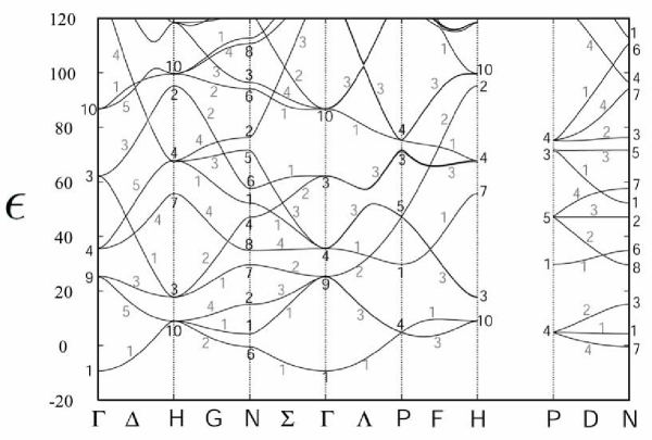
Figure 4: The band structures of P-surface. The numbers shown on each of the energy levels indicate the corresponding IR’s following the numbering scheme of Ref.ZakTables, . The numbers are shown in black for special points and in gray for special lines.

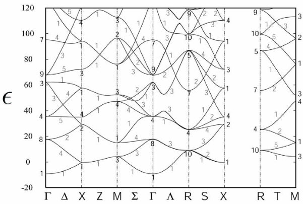
Figure 5: The band structures of D-surface. See the figure caption of Fig.4.

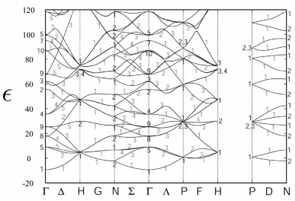
Figure 6: The band structures of G-surface. See the figure caption of Fig.4.

V Interrelation between the band structures

The crystallographic information given in Sec.III provides a basis for understanding the interrelations between the electronic structures of these TPMS’s. The boundary conditions for a dodecagonal patch of each surface is given as the phase factor multiplied upon translating it to any of its neighbors. The phase factor is given by $e^{2\pi i{\bf k}\cdot{\bf t}}$ for the translational vector ${\bf t}$, where ${\bf k}$ is the 3D wave vector. Instead of the 3D vectors ${\bf k}$ and ${\bf t}$, one can use the corresponding 6D vectors $\vec{k}$ and $\vec{t}$ which are restricted within the relevant 3D subspace. The phase factor is then rewritten as $e^{2\pi i\vec{k}\cdot\vec{t}}$, in which the vector $\vec{t}$ can safely be lifted to a 6D translational vector of $\Xi(w)$ prior to the orthogonal projection. The boundary conditions can be generalized further by allowing the vector $\vec{k}$, which should otherwise be restricted within the relevant 3D subspace for each surface, to take arbitrary values in the hypothetical 6D “reciprocal space”. Thus we are led to define the 6D band structures, $\hat{\epsilon}(\vec{k})$, which are periodic functions of the quasi-momentum, $\vec{k}=(k_{1},k_{2},k_{3},k_{4},k_{5},k_{6})$. Since $\hat{\epsilon}(\vec{k})$ are derived from the periodicity of $\Xi(w)$, they are periodic functions of $\vec{k}$ with the periodicity of $\Lambda^{\ast}$. It is understood that the band structures for each of the three TPMS’s are the section of $\hat{\epsilon}(\vec{k})$ along the relevant 3D subspace. Hence, if $\vec{k}_{X}$ is an arbitrary 6D vector along $E_{X}$ ($X=P,D,$ or $G$) and ${\bf k}_{X}$ is the 3D counterpart, then the band structures for X-surface is given as $\epsilon_{X}({\bf k}_{X})=\hat{\epsilon}(\vec{k}_{X})$.

It is readily shown that the intersection of a pair of subspaces, $E_{X}$ and $E_{Y}$ ($X,Y=P,D,$ or $G$), consists of just one point, which is at the origin. As a consequence, the energy eigenvalues of X-surface at $\Gamma$-point always coincide with those of Y-surface at $\Gamma$-point, because $\epsilon_{X}({\bf 0})=\epsilon_{Y}({\bf 0})=\hat{\epsilon}(\vec{0})$. In this case, we can say that the band structures of X- and Y-surfaces “intersect” at $\Gamma$-point.

A more general condition for the band intersection is given below. Recall $\hat{\epsilon}(\vec{k})$ has the periodicity of $\Lambda^{\ast}$, so that

$$\hat{\epsilon}(\vec{k}+\sum_{i}n_{i}\vec{Q}_{i})=\hat{\epsilon}(\vec{k}),$$ (32)

in which $n_{i}$ ($i=1,...,6$) are arbitrary integer coefficients. Therefore, if the two vectors $\vec{k}_{X}$ in $E_{X}$ and $\vec{k}_{Y}$ in $E_{Y}$ are connected through a scattering vector $\sum_{i}n_{i}\vec{Q}_{i}$ in $\Lambda^{\ast}$,

$$\vec{k}_{Y}=\vec{k}_{X}+\sum_{i}n_{i}\vec{Q}_{i},$$ (33)

then the relevant eigenvalues coincide, i.e., $\epsilon_{X}({\bf k}_{X})=\epsilon_{Y}({\bf k}_{Y})$. In particular, if $\sum_{i}n_{i}\vec{Q}_{i}\in\Lambda^{\ast}_{X}\oplus\Lambda^{\ast}_{Y}$, then one immediately finds that $\vec{k}_{X}\in\Lambda^{\ast}_{X}$ and $\vec{k}_{Y}\in\Lambda^{\ast}_{Y}$. Since these wave vectors are at the center of the Brillouin zones (BZ’s), the band intersection corresponds to $\Gamma$-point as discussed earlier. On the other hand, if $\sum_{i}n_{i}\vec{Q}_{i}$ does not belong to $\Lambda^{\ast}_{X}\oplus\Lambda^{\ast}_{Y}$, it is divided into two components in $E_{X}$ and $E_{Y}$ which are not at the center of the BZ’s. The latter case leads to band intersections at certain special points in the BZ’s. The total number of band intersections within the 6D BZ is given as the index $\mu$ of the sublattice $\Lambda^{\ast}_{X}\oplus\Lambda^{\ast}_{Y}$ in $\Lambda^{\ast}$.SublatticeIndex It can be shown that $\mu=4$ for the pair of P- and D-surfaces, 2 for that of P- and G-surfaces, and 1 for that of D- and G-surfaces. The corresponding band intersections occur at a set of special points in the BZ’s of these TPMS’s, as listed in TABLE 1. (For the derivation, see Appendix A.)

P-surface	D-surface	G-surface
$\Gamma$ ($\Gamma$,$H$)	$\Gamma$ ($\Gamma$,$R$)	$\Gamma$
$M$ $(N^{2})$	$X$ $(M,X)$
$R$ $(P^{2})$		$H$

Table 1: The list of the special points for the band intersections, as derived in Appendix A. The special points for the Bravais lattices of the dodecagonal unit patches are shown without parenthesis. The corresponding special points in the unfolded BZ’s for P- and D-surfaces are shown by parenthesis. A superscript is added if two special points in the same star correspond to a single band intersection.

The coincidence of energy eigenvalues as the result of band intersections are observed in our numerical results as demonstrated in Fig.7. This phenomenon has been found previously by Aoki et al.AKTMK01 ; KA05 in an empirical way. However, our theory provides a more clear account for this phenomenon in terms of the 6D algebra of Bonnet transformations. It also gives the exhaustive list of possible band intersections in TABLE 1. Moreover, the idea of band intersections can be applied generally to the band structures of TPMS’s connected via Bonnet transformations.

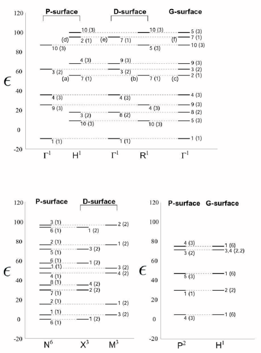
Figure 7: Energy diagrams showing the coincidence of energy levels at the special points listed in TABLE 1. The superscript for each special point symbol (e.g., N⁶) indicates the number of the equivalent points in the BZ, constituting the star. Each energy level is assigned the relevant IR, whose dimensionality is shown by parenthesis.

VI Symmetry analysis of the band structures

Symmetry has various implications in understanding the properties of materials involving the quantum mechanics of electrons. Dynamically, it implies the selection rules for quantum transitions or various forms of conservation laws. While statically, symmetry serves as the classification principle of structures and also provides basic clues for understanding the formation (or stability) of a particular material. It should also have significant implications in understanding the detailed characteristics of the present systems. Therefore, in the following, we shall carry out a detailed analysis on the symmetry aspects of the electronic structures of the TPMS’s.

A subspace of Bloch states $\phi_{\bf k}$ at a wave vector, ${\bf k}$, with an identical energy eigenvalue can be assigned an irreducible representation (IR) of $G_{\bf k}$, i.e., the group of ${\bf k}$. In practice, the representation matrices are obtained numerically, and are then analyzed by the use of the orthogonal relationships of IR’s.Lax ; TSPACE In fact, the discretization of the surfaces used for the numerical analysisAKTMK01 diminishes the space group, $G$, to $P4/mmm$, $P4_{2}/nnm$, and $I4_{1}/acd$ for P-, D-, and G-surfaces, respectively. Hence, for each surface, we can numerically analyze the IR’s only at ${\bf k}$-points whose group $G_{\bf k}$ are subgroups of the diminished space group. In addition, we may use the band branching rules (for instance, $\Gamma_{9}$ always splits into $\Delta_{3}$ and $\Delta_{5}$ for the space group $Im\bar{3}m$) to determine the IR’s for the rest of the ${\bf k}$ space. The numbers indicated on the band structure functions in Figs.4, 5, and 6 represent the relevant IR’s of $G_{\bf k}$; we comply with the numbering scheme given in Ref.ZakTables, . These IR’s describe the symmetry features of the relevant eigenstates. They also serve as criteria for the degeneracies in the band structures. This is useful since otherwise degenerate bands can slightly fall apart as artifacts of the diminishing of symmetry involved by the discretization procedure.

VI.1 Band sticking

Degeneracies occur due to several symmetry reasons. At high-symmetry special points in the BZ, we often observe several band energy curves sticking together into one energy level. The degeneracy of such an energy level is given by the dimensionality of the relevant IR. For the case of non-symmorphic space groups, the degeneracies at a special point on the boundary of the BZ can be larger than symmorphic counterparts when the transformation of eigenstates by $G_{\bf k}$ is represented as a multiplier group.Lax In the band structures of G-surface, for instance, we may observe relatively large degeneracies at H- and P-points; they are 6-fold (H₁), 4-fold (P₁), and 2-fold (H₂, H₃, H₄, P₂, P₃). Furthermore, we may find additional degeneracies due to the time-reversal symmetry on these special points.Herring ; Lax Namely, an energy level of the IR H₃ always sticks with one of the IR H₄, whereas the same holds for the pair of the IR’s, P₂ and P₃, both resulting in 4-fold degeneracies. Note the space group for G-surface, $Ia\bar{3}d$, is highly non-symmorphic including four-fold screw axes and two types of glide planes (one type is d-glide).

VI.2 Nodal lines

An interesting feature of the present systems is that, due to the 2D character of the surfaces, some of the eigenstates have nodal lines, i.e., lines along which an eigenstate has zero amplitude. Here, we shall study the occurrence of nodal lines in somewhat detail from the symmetry standpoint, because nodal lines have the following significant implications for the electronic properties. Firstly, the density of nodal lines is correlated with the magnitude of energy eigenvalue. Secondly, nodal lines occur as a consequence of the quantum interference of an electronic wave and are closely related to the symmetry and topology of the surfaces.

There is an important class of nodal lines which can be understood in terms of the symmetry properties of the eigenstates; a nodal line should appear when the relevant IR has odd parity with respect to a symmetry element which leaves the positions of the nodal line invariant. There are two types of such symmetry elements: mirrors (a nodal line will appear at the intersection between the surface and a mirror plane) and two-fold axes lying in the surface (a nodal line will appear along such an axis).

In the space group $Im\bar{3}m$ of P-surface, the symmetry elements related to the generation of nodal lines are

• (two-fold axes $U_{d}$) $U^{xy}$, $U^{\bar{x}y}$, $U^{yz}$, $U^{\bar{y}z}$, $U^{zx}$, $U^{\bar{z}x}$,

• (mirrors $\sigma_{d}$) $\sigma^{xy}$, $\sigma^{\bar{x}y}$, $\sigma^{yz}$, $\sigma^{\bar{y}z}$, $\sigma^{zx}$, $\sigma^{\bar{z}x}$,

• (mirrors $\sigma$) $\sigma^{x}$, $\sigma^{y}$, $\sigma^{z}$.

Note that the elements of the factor group are implied by the symbols of point group elements. Throughout this paper, the symbols of point group elements comply with those used in Ref.ZakTables, . One can find that the above three types of symmetry operations leave the high-symmetry geodesics on P-surface, i.e., $\alpha$-, $\beta$-, and $\gamma$-type geodesics as defined in Fig.2, invariant. The correspondence between the types of symmetry operations and those of geodesics are given by $\alpha\leftrightarrow U_{d}$, $\beta\leftrightarrow\sigma_{d}$, and $\gamma\leftrightarrow\sigma$ (see Fig.1).

A similar list for D-surface (space group $Pn\bar{3}m$) is given as

• (mirrors $\sigma_{d}$) $\sigma^{xy}$, $\sigma^{\bar{x}y}$, $\sigma^{yz}$, $\sigma^{\bar{y}z}$, $\sigma^{zx}$, $\sigma^{\bar{z}x}$,

• (two-fold axes $U_{d}$) $U^{xy}$, $U^{\bar{x}y}$, $U^{yz}$, $U^{\bar{y}z}$, $U^{zx}$, $U^{\bar{z}x}$,

• (two-fold axes $U$) $U^{x}$, $U^{y}$, $U^{z}$.

In this case the correspondence is established as, $\alpha\leftrightarrow\sigma_{d}$, $\beta\leftrightarrow U_{d}$, and $\gamma\leftrightarrow U$ (see Fig.1).

On the other hand, no such symmetry elements exist for G-surface, that is, there are no mirror planes (though there are several glide planes) nor two-fold axes lying in the surface. Hence no nodal lines are predicted by symmetry for G-surface.

It is deducible from the character table of a given ${\bf k}$-point in the BZ whether a given IR entails any nodal lines by symmetry. One can consult the character tables for the space groups in Ref.ZakTables, . It is necessary from the previous paragraph that the group of ${\bf k}$, $G_{\bf k}$, contains at least one symmetry element(s) responsible for the generation of nodal lines. Then, if an IR of $G_{\bf k}$ has odd parity with respect to those symmetry elements, a nodal line will appear accordingly. One should bear in mind that the representative of the relevant factor group $(\gamma|{\bf c})$ ($\gamma$ is the point group operation and ${\bf c}$ the additional translation, which is usually taken to be zero when the space group is symmorphic) does not necessarily leave the position of the nodal line invariant. Instead, one should consider $(\gamma|{\bf r})$ with

$${\bf r}={\bf q}-\gamma{\bf q}={\bf c}-{\bf R}_{\bf q}^{(\gamma|{\bf c})},$$ (34)

where ${\bf q}$ is any position in the relevant mirror or axis. Here, ${\bf R}_{\bf q}^{(\gamma|{\bf c})}=(\gamma|{\bf c}){\bf q}-{\bf q}$ is always a Bravais vector. The relevant matrix for $(\gamma|{\bf r})$ is given by

$$D[(\gamma|{\bf r})]=\exp{[-i{\bf kR}_{\bf q}^{(\gamma|{\bf c})}]}D[(\gamma|{\bf c})].$$ (35)

Therefore, in order to discern the parity of an IR at the position of a nodal line, the character for the representative element of the relevant factor group (the value given in the character table) should be multiplied by $\exp{[-i{\bf kR}_{\bf q}^{(\gamma|{\bf c})}]}$. The exhaustive lists of IR’s which entail nodal lines by the above argument are given in TABLES 2 and 3 for P- and D-surfaces, respectively. For each of the IR’s listed, the corresponding nodal lines are given by parenthesis.

${\bf k}$-point	$G_{k}/T$	IR (nodal lines)
$\Gamma~{}(0,0,0)$	$O_{h}$	$\Gamma_{2}(6U_{d},6\sigma_{d}),\Gamma_{6}(3\sigma,6\sigma_{d}),\Gamma_{7}(6U_{d},3\sigma),\Gamma_{8}(3\sigma)$
$\Delta~{}(k_{x},0,0)$	$C_{4v}$	$\Delta_{2}(2\sigma,2\sigma_{d}),\Delta_{3}(2\sigma_{d}),\Delta_{4}(2\sigma)$
$H~{}(1,0,0)$	$O_{h}$	$H_{1}(6U_{d}),H_{2}(6\sigma_{d}),H_{6}(6U_{d},3\sigma,6\sigma_{d}),H_{7}(3\sigma),H_{8}(3\sigma)$
$\Sigma~{}(k_{x},k_{x},0)$	$C_{2v}$	$\Sigma_{2}(U_{d},\sigma_{d}),\Sigma_{3}(\sigma,\sigma_{d}),\Sigma_{4}(U_{d},\sigma)$
$G~{}(k_{x},1-k_{x},0)$	$C_{2v}$	$G_{1}(U_{d}),G_{2}(\sigma_{d}),G_{3}(U_{d},\sigma,\sigma_{d}),G_{4}(\sigma)$
$N~{}(\frac{1}{2},\frac{1}{2},0)$	$D_{2h}$	$N_{1}(U^{\bar{x}y}),N_{2}(\sigma^{\bar{x}y},\sigma^{z}),N_{3}(U^{xy},U^{\bar{x}y},\sigma^{z},\sigma^{xy}),N_{4}(U^{xy},\sigma^{xy},\sigma^{\bar{x}y}),$
		$N_{5}(U^{\bar{x}y},\sigma^{z},\sigma^{xy},\sigma^{\bar{x}y}),N_{6}(\sigma^{xy}),N_{7}(U^{xy},U^{\bar{x}y},\sigma^{\bar{x}y}),N_{8}(U^{xy},\sigma^{z})$
$\Lambda~{}(k_{x},k_{x},k_{x})$	$C_{3v}$	$\Lambda_{2}(3\sigma_{d})$
$F~{}(k_{x},1-k_{x},1-k_{x})$	$C_{3v}$	$F_{2}(3\sigma_{d})$
$D~{}(\frac{1}{2},\frac{1}{2},k_{z})$	$C_{2v}$	$D_{2}(\sigma^{xy}),D_{3}(\sigma^{xy},\sigma^{\bar{x}y}),D_{4}(\sigma^{\bar{x}y})$
$P~{}(\frac{1}{2},\frac{1}{2},\frac{1}{2})$	$T_{d}$	$P_{2}(6\sigma_{d})$
$\Xi~{}(k_{x},k_{y},0)$	$C_{s}$	$\Xi_{2}(\sigma)$
$\Theta~{}(k_{x},k_{x},k_{z})$	$C_{s}$	$\Theta_{2}(\sigma_{d})$
$B~{}(k_{x},1-k_{x},k_{z})$	$C_{s}$	$B_{2}(\sigma_{d})$

Table 2: The list of the IR’s for P-surface ($Im\bar{3}m$) entailing nodal lines by symmetry. The IR’s shown have odd parity with respect to the symmetry elements given by parenthesis; these elements are of the types, $U_{d}$, $\sigma_{d}$, and $\sigma$, which are responsible for the generation of nodal lines along $\alpha$-, $\beta$-, and $\gamma$-geodesics, respectively. A set of symmetrically equivalent elements are shown by the numbered type symbols; e.g., $3\sigma=\{\sigma_{x},\sigma_{y},\sigma_{y}\}$.

${\bf k}$-point	$G_{k}/T$	IR (nodal lines)
$\Gamma~{}(0,0,0)$	$O_{h}$	$\Gamma_{2}(6U_{d},6\sigma_{d}),\Gamma_{6}(6\sigma_{d}),\Gamma_{7}(6U_{d})$
$\Delta~{}(k_{x},0,0)$	$C_{4v}$	$\Delta_{2}(2\sigma_{d}),\Delta_{3}(2\sigma_{d}),\Delta_{5}(U)$
$X~{}(\frac{1}{2},0,0)$	$D_{4h}$	$X_{2}(2\sigma_{d}),X_{3}(U^{x},U^{yz},U^{\bar{y}z}),X_{4}(U^{x})$
$\Sigma~{}(k_{x},k_{x},0)$	$C_{2v}$	$\Sigma_{2}(\sigma_{d},U_{d}),\Sigma_{3}(\sigma_{d}),\Sigma_{4}(U_{d})$
$Z~{}(k_{x},\frac{1}{2},0)$	$C_{2v}$	—
$M~{}(\frac{1}{2},\frac{1}{2},0)$	$D_{4h}$	$M_{1}(U^{z}),M_{2}(U^{z},2\sigma_{d}),M_{4}(U^{xy},U^{\bar{x}y})$
$\Lambda~{}(k_{x},k_{x},k_{x})$	$C_{3v}$	$\Lambda_{2}(3\sigma_{d})$
$S~{}(\frac{1}{2},k_{y},k_{y})$	$C_{2v}$	$S_{3}(\sigma^{\bar{y}z}),S_{4}(\sigma^{\bar{y}z})$
$T~{}(\frac{1}{2},\frac{1}{2},k_{z})$	$C_{4v}$	$T_{2}(U^{z}),T_{3}(U^{z}),T_{4}(U^{z}),T_{5}(U^{z})$
$R~{}(\frac{1}{2},\frac{1}{2},\frac{1}{2})$	$O_{h}$	$R_{1}(3U,6U_{d}),R_{2}(3U,6\sigma_{d}),R_{3}(3U),R_{6}(3U,6U_{d},6\sigma_{d}),R_{7}(3U),R_{8}(3U)$
$\Xi~{}(k_{x},k_{y},0)$	$C_{s}$	—
$\Theta~{}(k_{x},k_{x},k_{z})$	$C_{s}$	$\Theta_{2}(\sigma_{d})$
$A~{}(\frac{1}{2},k_{y},k_{z})$	$C_{s}$	—

Table 3: The list of the IR’s for D-surface ($Pn\bar{3}m$) entailing nodal lines by symmetry. The IR’s shown have odd parity with respect to the symmetry elements of the types, $\sigma_{d}$, $U_{d}$, and $U$, which are responsible for the generation of nodal lines along $\alpha$-, $\beta$-, and $\gamma$-geodesics, respectively.

For G-surface, we may still find related nodal lines for eigenstates on the special points $\Gamma$ and $H$, corresponding to band intersections. These eigenstates are in one-to-one correspondence with eigenstates of P- and D-surfaces on the relevant special points (see also a discussion in Sec.VII), and they are identical intrinsically within the dodecagonal unit patch. Therefore if some nodal lines are present for symmetry reasons for P- and D-surfaces, the corresponding states of G-surface should also have nodal lines. Illustrative examples are given in Fig.8, which shows two sets of eigenstates with IR’s {$H_{7}$, $R_{7}$, $\Gamma_{2}$} and {$H_{2}$, $\Gamma_{7}$, $\Gamma_{7}$} for {P, D, G}-surfaces, respectively. One can see that the sets of nodal lines are intrinsically the same within each set.

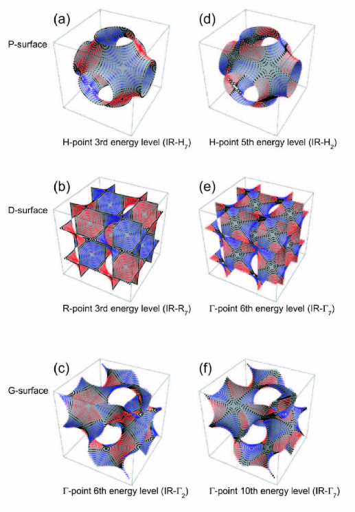
Figure 8: (Color) In each column eigenstates with identical energy eigenvalue corresponding to a band intersection are shown. The dots are the actual mesh points for the numerical calculation. Opposite signs of the wave functions are indicated by the blue and red colors, while the black dots indicate the amplitude whose absolute value is close to zero, corresponding to the nodal lines. The states in the set {(a), (b), (c)} have nodal lines along all the $\gamma$ type geodesics, while ones in the set {(d), (e), (f)} have nodal lines along all the $\beta$ type geodesics. The $\gamma$ type geodesics for G-surface in (c) constitute the helical lines of both chirality along $x$, $y$, and $z$ directions .

We find that some eigenstates have nodal lines which do not correspond to any of the three types of high symmetry geodesics. This kind of nodal lines are by no means easy to predict because they are not directly related to mirrors nor two-fold axes in the surface. However, such nodal lines would appear only at sufficiently high energies.

VII Discussions

The idea of band intersections discussed in Sec.V can be paraphrased in the following way. The Bloch condition for the eigenstates of a crystal is given as the proper phase relationships of the reference unit cell to its neighbors. For the present case, we have shown that the phase relationships of a dodecagonal unit to its twelve neighbors become identical between two different surfaces at the k points of a band intersection. Therefore, the partial Hamiltonians $h_{\bf k}$ acting on the subspaces of states at these k points will become equivalent. The coincidence of energy eigenvalues is just a result of this fact. If there are several members in the star of the special points, all these members give a set of symmetrically equivalent phase relationships of the dodecagonal unit patch; for instance, the stars of M-point (s.c.) of P-surface and X-point (f.c.c.) of D-surface forming band intersections are three membered. Except for at the band intersections, the phase relationships cannot coincide among the three surfaces because of their topological differences.

The equivalence of partial Hamiltonians $h_{\bf k}$ between two surfaces at a band intersection implies a one-to-one correspondence between the subspaces of states of the same energy level. If the two sides of the surfaces are distinct, the correspondence would be simple so that one could expect a one-to-one correspondence between the IR’s between the surfaces. However, as we see in Fig.7, the correspondence is somewhat obscure due to the reduction of the primitive unit cells for P- and D-surfaces when the two sides are indistinguishable. The unfolding of the BZ’s for these two surfaces results in the splitting of a single band intersection in the 6D BZ into two different special points (see TABLE 1). The resulting two special points can either be (i) equivalent, as in the case of two $N$-points for P-surface, or (ii) inequivalent, as in the case of $\Gamma$- and $H$-points for P-surface. For the case (i), a subspace of states at a band intersection is divided into two subspaces associated with the two k points in the same star, so that the dimensionality of the IR’s is reduced by half from that of the original subspace. Meanwhile, in the case (ii), a subspace of states at a band intersection is mapped onto a single subspace associated with either of the different special points. This argument is based on that each subspace at a single k point is in general associated with a single IR, and that the total dimensionality of the original subspaces at a band intersection is identical between the relevant two surfaces.

We expect that there is a certain connection between the IR’s of different surfaces at their band intersections. It appears that an IR of P-surface corresponds uniquely to an IR of D-surface, while an IR of G-surface corresponds to two IR’s of P-surface as well as D-surface. In Fig.7 one finds that the IR $\Gamma_{9}$ of G-surface corresponds to either $\Gamma_{9}$ or $H_{4}$ of P-surface as well as to either $\Gamma_{9}$ or $R_{4}$ of D-surface. Interestingly, the connection between the IR’s of P-surface at $P$-point and those of G-surface at $H$-point can be uniquely determined by the dimensionality of the IR’s as

$$P_{1}(1),P_{2}(1) \leftrightarrow H_{2}(2),$$

$$P_{3}(2) \leftrightarrow H_{3}+H_{4}(2+2),$$

$$P_{4}(3),P_{5}(3) \leftrightarrow H_{1}(6),$$

where the dimensionality of each IR is denoted by parenthesis. (Recall that the IR’s $H_{3}$ and $H_{4}$ for G-surface is degenerate due to the time-reversal symmetry.) For rigorous proofs of the general relationships between the IR’s of the three surfaces, more detailed investigations on the group theoretical aspects of the problem may be required. Still, our results can be a starting point for further studies.

The relationship between the symmetry properties of eigenstates and the occurrence of nodal lines are established in Sec.VI. The existence of nodal lines in an eigenstate necessitate a sufficient amount of kinetic energy, so that IR’s with a large number of nodal lines cannot appear in a lowest part of the energy spectrum. In TABLES 2 and 3, one can find that the following IR’s accompany a significant number of nodal lines: {$\Gamma_{2}$, $\Gamma_{6}$, $\Gamma_{7}$, $H_{6}$} of P-surface and {$\Gamma_{2}$, $R_{1}$, $R_{2}$, $R_{6}$} of D-surface. These IR’s are naturally absent in Figs.4 and 5. It is also seen that IR’s with nodal lines appear roughly in the increasing order in the number of nodal lines as one goes up the energy axis. Therefore, nodal lines can be regarded as an important feature of eigenstates present in real-space in order to understand the overall characteristics of the systems.

For a full account of the electronic structures of the present systems, a more detailed study on the topological aspects of the problem should be important. Due to the topological characters of the surfaces, there may be a “topological invariant” associated with the continuum of eigenstates along a dispersion curve in the band structures. Such a topological invariant might be given as the phase winding numbers associated with characteristic closed paths on the surface. The topological characters of the eigenstates may explain the connectivity aspects of the energy bands. Further properties of the energy bands (e.g., the flatness, particle-/hole-type dispersions) might also be explained based on real-space pictures of the relevant eigenstates.

It is instructive to note that the arguments throughout this paper are not binded by the particular form of the curvature potential as long as it is determined intrinsically. Hence, by generalizing the potential to any function of the Gaussian curvature one may be able to deal with secondary effects of curvatures, such as the effect of varying thickness of the surface depending on the curvatures.

In summary, we have studied in detail the band structures of the strongly constrained electron systems onto P-, D-, and G-surfaces. The crystallographic relations of these surfaces in six dimensions have proved to be useful in understanding the interrelations between the electronic structures of these surfaces. By introducing the hypothetical 6D band structures, the coincidence of eigenstates among different surfaces at particular sets of k points has been explained in terms of the idea of band intersections. We have given the exhaustive list of band intersections for the three surfaces. A numerical investigation of the band structures with a detailed analysis of the symmetry properties has also been performed. We have assigned IR’s of the space groups to the energy bands displayed in Figs.4,5, and 6. As a key feature to understand the consequences of the symmetry of the eigenstates, the occurrence of characteristic nodal lines have been discussed somewhat in detail. We have given the conditions for nodal lines to be predicted by symmetry and also the exhaustive lists of IR’s which entail nodal lines for P- and D-surfaces.

*

Appendix A The index of $\Lambda^{\ast}_{X}\oplus\Lambda^{\ast}_{Y}$ in $\Lambda^{\ast}$

We consider the sublattices of $\Lambda^{\ast}$ given in the form $\Lambda_{X}^{\ast}\oplus\Lambda_{Y}^{\ast}$ ($X,Y=P,D$, or $G$). From Eq.(28), it is straightforward to obtain the following:

$$\Lambda^{\ast}_{P}\oplus\Lambda^{\ast}_{D} = \left\{~{}i~{}(\vec{Q}_{1}+\vec{Q}_{5}-\vec{Q}_{6})+j~{}(\vec{Q}_{2}-\vec{Q}_{4}+\vec{Q}_{6})+k~{}(\vec{Q}_{3}+\vec{Q}_{4}-\vec{Q}_{5})\right.$$ (36)

$$\left.+~{}l~{}(-\vec{Q}_{2}+\vec{Q}_{3}+\vec{Q}_{4})+m~{}(\vec{Q}_{1}-\vec{Q}_{3}+\vec{Q}_{5})+n~{}(-\vec{Q}_{1}+\vec{Q}_{2}+\vec{Q}_{6})~{}\right\},$$

$$\Lambda^{\ast}_{P}\oplus\Lambda^{\ast}_{G} = \left\{~{}i~{}(\vec{Q}_{1}+\vec{Q}_{5}-\vec{Q}_{6})+j~{}(\vec{Q}_{2}-\vec{Q}_{4}+\vec{Q}_{6})+k~{}(\vec{Q}_{3}+\vec{Q}_{4}-\vec{Q}_{5})\right.$$ (37)

$$\left.+~{}l~{}(\vec{Q}_{1}-\vec{Q}_{4}-\vec{Q}_{6})+m~{}(\vec{Q}_{2}-\vec{Q}_{4}-\vec{Q}_{5})+n~{}(\vec{Q}_{3}-\vec{Q}_{5}-\vec{Q}_{6})~{}\right\},$$

$$\Lambda^{\ast}_{D}\oplus\Lambda^{\ast}_{G} = \left\{~{}i~{}(-\vec{Q}_{2}+\vec{Q}_{3}+\vec{Q}_{4})+j~{}(\vec{Q}_{1}-\vec{Q}_{3}+\vec{Q}_{5})+k~{}(-\vec{Q}_{1}+\vec{Q}_{2}+\vec{Q}_{6})\right.$$ (38)

$$\left.+~{}l~{}(\vec{Q}_{1}-\vec{Q}_{4}-\vec{Q}_{6})+m~{}(\vec{Q}_{2}-\vec{Q}_{4}-\vec{Q}_{5})+n~{}(\vec{Q}_{3}-\vec{Q}_{5}-\vec{Q}_{6})~{}\right\},$$

where $i$, $j$, $k$, $l$, $m$, and $n$ are arbitrary integers. In the following, the orthonormal basis sets of the 3D subspaces $E_{P}$, $E_{D}$, and $E_{G}$ are denoted as $\vec{e}_{P,i}$, $\vec{e}_{D,i}$ and $\vec{e}_{G,i}$ ($i=1,2,3$), respectively. These basis vectors are obtained as the row vectors of the corresponding orthogonal projectors, $\Pi_{P}$, $\Pi_{D}$, and $\Pi_{G}$.

A.1 $\Lambda^{\ast}_{P}\oplus\Lambda^{\ast}_{D}$

$\Lambda^{\ast}_{P}\oplus\Lambda^{\ast}_{D}$ is the sublattice of $\Lambda^{\ast}=\{\sum^{6}_{i=1}n_{i}\vec{Q}_{i}\}$ for which the coefficients $n_{i}$ are given by

$$\left(\begin{array}[]{c}n_{1}\\ n_{2}\\ n_{3}\\ n_{4}\\ n_{5}\\ n_{6}\end{array}\right)={\bf M}_{PD}\left(\begin{array}[]{c}i\\ j\\ k\\ l\\ m\\ n\end{array}\right),\quad{\bf M}_{PD}=\left(\begin{array}[]{cccccc}1&0&0&0&1&-1\\ 0&1&0&-1&0&1\\ 0&0&1&1&-1&0\\ 0&-1&1&1&0&0\\ 1&0&-1&0&1&0\\ -1&1&0&0&0&1\end{array}\right).$$ (57)

Since the index $|\det{\bf M}_{PD}|=4$, $\Lambda^{\ast}$ is divided into four sublattices equivalent to $\Lambda^{\ast}_{P}\oplus\Lambda^{\ast}_{D}$. Each sublattice is specified by a pair of indices, ($p,q$):

$$p = n_{1}+n_{3}+n_{4}+n_{6}\mod{2},$$ (58)

$$q = n_{2}+n_{3}+n_{5}+n_{6}\mod{2}.$$ (59)

In particular, the sublattice $\Lambda^{\ast}_{P}\oplus\Lambda^{\ast}_{D}$ is specified by ($p=0$, $q=0$). It gives rise to the band intersection at $\Gamma$-point, $\vec{k}_{P}=\vec{k}_{D}=\vec{0}$, in Eq.(33). The other three sublattices are obtained by translating $\Lambda^{\ast}_{P}\oplus\Lambda^{\ast}_{D}$ by $\vec{Q}_{1}$ ($p=1,q=0$), $\vec{Q}_{2}$ ($p=0,q=1$), and $\vec{Q}_{3}$ ($p=1,q=1$). For each of these sublattices, the vectors $\vec{k}_{P}$ and $\vec{k}_{D}$ in Eq.(33) can be taken as

$$\vec{k}_{P}=(\vec{e}_{P,2}+\vec{e}_{P,3})/(2r\ell),\,\vec{k}_{D}=(\vec{e}_{D,2}-\vec{e}_{D,3})/(2s\ell)$$

$$\qquad{\rm for}~{}p=1,q=0\quad(\vec{k}_{P}-\vec{k}_{D}=\vec{Q}_{1}),$$ (60)

$$\vec{k}_{P}=(\vec{e}_{P,1}+\vec{e}_{P,3})/(2r\ell),\,\vec{k}_{D}=(-\vec{e}_{D,1}+\vec{e}_{D,3})/(2s\ell)$$

$$\qquad{\rm for}~{}p=0,q=1\quad(\vec{k}_{P}-\vec{k}_{D}=\vec{Q}_{2}),$$ (61)

$$\vec{k}_{P}=(\vec{e}_{P,1}+\vec{e}_{P,2})/(2r\ell),\,\vec{k}_{D}=(\vec{e}_{D,1}-\vec{e}_{D,2})/(2s\ell)$$

$$\qquad{\rm for}~{}p=1,q=1\quad(\vec{k}_{P}-\vec{k}_{D}=\vec{Q}_{3}).$$ (62)

It is readily shown that these three band intersections are observed at the three membered star of M-point in the BZ of P-surface as well as at the three membered star of X-point in the BZ of D-surface, where the dodecagonal patches are taken as the primitive cells.

A.2 $\Lambda^{\ast}_{P}\oplus\Lambda^{\ast}_{G}$

A similar argument holds for $\Lambda^{\ast}_{P}\oplus\Lambda^{\ast}_{G}$, for which

$${\bf M}_{PG}=\left(\begin{array}[]{cccccc}1&0&0&1&0&0\\ 0&1&0&0&1&0\\ 0&0&1&0&0&1\\ 0&-1&1&-1&-1&0\\ 1&0&-1&0&-1&-1\\ -1&1&0&-1&0&-1\end{array}\right).$$ (69)

The index is $|\det{\bf M}_{PG}|=2$. Hence, there are two equivalent sublattices specified by an index, $r$:

$$r=n_{4}+n_{5}+n_{6}\mod{2}.$$ (70)

Apart from the trivial band intersection for $r=0$ at $\Gamma$-point, we have another band intersection for the sublattice $r=1$, which is obtained by translating $\Lambda^{\ast}_{P}\oplus\Lambda^{\ast}_{G}$ by $\vec{Q}_{4}$. The relevant vectors $\vec{k}_{P}$ and $\vec{k}_{G}$ can be taken as

$$\vec{k}_{P}=(\vec{e}_{P,1}-\vec{e}_{P,2}+\vec{e}_{P,3})/(2r\ell),\,\vec{k}_{G}=\vec{e}_{G,1}/(2b\ell)$$

$$\qquad{\rm for}~{}r=1\quad(\vec{k}_{P}-\vec{k}_{G}=\vec{Q}_{4}).$$ (71)

The band intersection is therefore observed at R-point in the BZ of P-surface as well as at H-point in that of the G-surface, where the dodecagonal patches are taken as the primitive cells.

A.3 $\Lambda^{\ast}_{D}\oplus\Lambda^{\ast}_{G}$

For $\Lambda^{\ast}_{D}\oplus\Lambda^{\ast}_{G}$,

$${\bf M}_{DG}=\left(\begin{array}[]{cccccc}0&1&-1&1&0&0\\ -1&0&1&0&1&0\\ 1&-1&0&0&0&1\\ 1&0&0&-1&-1&0\\ 0&1&0&0&-1&-1\\ 0&0&1&-1&0&-1\end{array}\right).$$ (78)

The index is $|\det{\bf M}_{DG}|=1$. Therefore $\Lambda^{\ast}_{D}\oplus\Lambda^{\ast}_{G}=\Lambda^{\ast}$, and there is no extra band intersection other than the trivial one at $\Gamma$-point.

References

- (1) H. G. von Schnering and R. Nesper, Z. Phys. B: Condensed Matter 83, 407 (1991).
- (2) S. Andersson, S. T. Hyde, K. Larsson, and S. Lidin, Chem. Rev. 88, 221 (1988).
- (3) H. Jensen and H. Koppe, Ann. Phys. 63, 586 (1971).
- (4) R. C. T. da Costa, Phys. Rev. A 23, 1982 (1981).
- (5) R. C. T. da Costa, Phys. Rev. A 25, 2893 (1982).
- (6) M. Ikegami and Y. Nagaoka, Prog. Theor. Phys. Suppl. 106, 235 (1991).
- (7) P. Duclos and P. Exner, Rev. Math. Phys. 7, 73 (1995).
- (8) G. Carron, P. Exner, and D. Krejcirik, J. Math. Phys. 45, 774 (2004).
- (9) N. L. Balazs and A. Voros, Phys. Rep. 143, 109 (1986).
- (10) H. Aoki, M. Koshino, D. Takeda, H. Morise, and K. Kuroki, Phys. Rev. B 65, 035102 (2001).
- (11) M. Koshino and H. Aoki, Phys. Rev. B 71, 073405 (2005).
- (12) M. Spivak, A Comprehensive Introduction to Differential Geometry (Publish or Perish, Berkeley, 1975), Vols. 3 and 4.
- (13) R. Osserman, A Survey of Minimal Surfaces (Dover, 1986).
- (14) Different minimal surfaces which just differ by the Bonnet angles, , in Eq.(1) constitute a Bonnet family.
- (15) J. Charvolin and J.-F. Sadoc, J. Phys. (Paris) 48, 1559 (1987).
- (16) J.-F. Sadoc and J. Charvolin, Acta Cryst. A 45, 10-20 (1989).
- (17) H. Schwarz, Gesammelte Mathematische Abhandlungen (Springer, Berlin, 1890), vol.1.
- (18) A. H. Schn, NASA Technical Report TN D-5541 (Washington DC, 1970).
- (19) The Riemann surface consists of two sheets of complex plane with four branch cuts, and it corresponds to the unit cell of each TPMS.
- (20) P. J. F. Gandy, D. Cvijovi, A. L. Mackay, and J. Klinowski, Chem. Phys. Lett. 314, 543 (1999); P. J. F. Gandy and J. Klinowski, Chem. Phys. Lett. 321, 363 (2000); Chem. Phys. Lett. 322, 579 (2000).
- (21) A () triangle is a triangle bounded by geodesics with the internal angles, (). Since the surfaces have negative Gaussian curvatures, the Gauss-Bonnet theorem requires the sum of these angles to be smaller than .
- (22) C. Oguey and J.-F. Sadoc, J. Phys. I France 3, 839 (1993).
- (23) In general, the curvature potential at any given point depends not only on the intrinsic curvatures but also on the extrinsic ones. Hence, the problem is essentially distinct from the classical counterpart, as discussed in Ref. C81, ).
- (24) This means that is divided into equivalent sublattices congruent to .
- (25) M. Lax, Symmetry Principles in Solid State and Molecular Physics (Wiley, New York, 1974).
- (26) A. Yanase, Fortran Program for Space Group (TSPACE) (Shokabo, Tokyo, 1995).
- (27) J. Zak, A. Casher, M. Glck, and Y. Gur, The Irreducible Representations of Space Groups (Benjamin, New York, 1969).
- (28) C. Herring, Phys. Rev. 52, 361 (1937).