Multi-state Epidemic Processes on Complex Networks

Abstract

Abstract: Infectious diseases are practically represented by models with multiple states and complex transition rules corresponding to, for example, birth, death, infection, recovery, disease progression, and quarantine. In addition, networks underlying infection events are often much more complex than described by meanfield equations or regular lattices. In models with simple transition rules such as the SIS and SIR models, heterogeneous contact rates are known to decrease epidemic thresholds. We analyze steady states of various multi-state disease propagation models with heterogeneous contact rates. In many models, heterogeneity simply decreases epidemic thresholds. However, in models with competing pathogens and mutation, coexistence of different pathogens for small infection rates requires network-independent conditions in addition to heterogeneity in contact rates. Furthermore, models without spontaneous neighbor-independent state transitions, such as cyclically competing species, do not show heterogeneity effects.

I Introduction

Many epidemic systems can be represented as a graph where vertices stand for individuals and an edge connecting a pair of vertices indicates interaction between individuals. Since late 1990s, real networks underlying disease transmission have been recognized to be complex and not approximated by conventional graphs such as lattices, regular trees, or classical random graphs. Not only being complex, many networks have the small-world and scale-free properties Albert02 ; NewmanSIAM . An important property of small-world networks is that the distance between a pair of vertices, or the minimum number of edges connecting two vertices, is fairly small on average. The scale-free property means that the vertex degree $k$, or the number of contacts with other individuals (vertices) for a given individual, has a power law distribution: $p_{k}\propto k^{-\gamma}$ Barabasi99 . Typically, $\gamma$ ranges between 2 and 3 Albert02 ; NewmanSIAM . In contrast, the degree is uniform on, for example, the square lattice ($k=4$).

Extending earlier data on heterogeneous sexual contact rates of humans Hethcote84 ; Anderson86 ; May88TRANS , current real data support that scale-free networks underly propagation of sexually transmitted diseases such as gonorrhea, genital herpes, HIV Colgate ; Andersonbook ; Liljeros ; Schneeberger , and computer viruses Pastor01PRL ; Pastorbook ; NewmanSIAM . Theoretically, epidemic thresholds above which epidemic outbreaks or endemic states ensue scale as $\left<k\right>/\left<k^{2}\right>$. Here $\left<k\right>\equiv\sum_{k=1}^{\infty}kp_{k}$ is the mean degree, and $\left<k^{2}\right>\equiv\sum_{k=1}^{\infty}k^{2}p_{k}$ is the second moment of the degree. Then a heterogeneous population, which has a large $\left<k^{2}\right>$ in comparison with $\left<k\right>$, yields a smaller epidemic threshold and are more likely to elicit outbreaks. Particularly, scale-free networks with $\gamma\leq 3$ have epidemic thresholds equal to 0 because $\left<k^{2}\right>$ diverges. Then, disease propagation on a global scale can occur for an arbitrary small infection rate. This holds for the percolation Albert00NAT ; Callaway00 ; Cohen00PRL ; Newman02_bond , the contact process (also called the SIS model) that describes endemic diseases such as gonorrhea Hethcote84 ; Pastor01PRL ; Pastor01PRE , and the SIR model that describes single-shot outbreak dynamics such as HIV Anderson86 ; May88TRANS ; May01 ; Moreno02EPB .

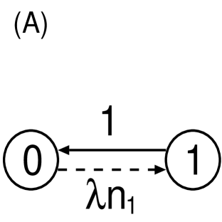
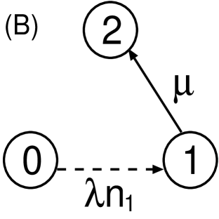
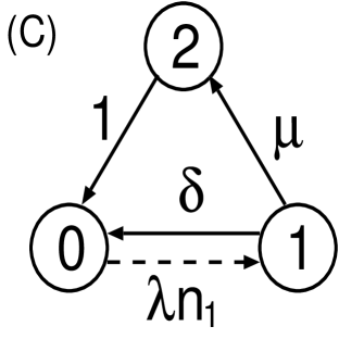
Figure 1: The state-transition rules of (A) the contact process, (B) the SIR model, and (C) the SIRS model. Solid lines represent transitions independent of states of neighbors. Dashed lines represent neighbor-dependent transitions. The values indicate the transmission rates, where $n_{i}$ is the number of neighbors with state $i$.

Apart from heterogeneous contact rates, realistic epidemic processes are also more complex than merely described by the percolation, the contact process, or the SIR model. Practical epidemic models often have more detailed states corresponding to, for example, exposed, quarantine, and mutated. Accordingly, state-transition rules become more complicated Hethcote84 ; May88TRANS ; Andersonbook ; Hopbauerbook . It is convenient to represent the transition rules of an epidemic model by a schematic figure like Fig. 1. Solid lines mean state-transition routes whose event rates are independent of the states of neighbors (e.g. death, recovery, mutation). Dashed lines represent ones whose rates are proportional to the neighbors’ states (e.g. reproduction, infection). Then, the contact process and the SIR model are represented by Fig. 1(A) and 1(B), respectively. For example, in the contact process, a susceptible individual (state 0) turns infected (state 1) at a rate proportional to the number of infected individuals in the neighborhood $(=n_{1})$. The infection rate is denoted by $\lambda$, and the spontaneous recovery rate is set equal to unity.

Understanding of multi-state contagion models on complex networks may be helpful in combatting real epidemics. In this direction, Liu and coworkers analyzed the SIRS model, which has the state of partial immunity R and is schematically shown in Fig. 1(C) Liu04JSM . They also studied the household model, in which each vertex has a graded state corresponding to the number of patients in a household Liu04PHA . They showed that the epidemic thresholds are proportional to $\left<k\right>/\left<k^{2}\right>$ also in these models. However, how general the universality of the $\left<k\right>/\left<k^{2}\right>$-scaling is has not been addressed.

In this paper, we analyze various multi-state epidemic processes originally proposed for lattices or populations with homogeneous contact rates. We concentrate on endemic models in which the phase boundary between the coexistence state, where both susceptible and infected individuals can survive, and the disease-free state with the susceptible individuals only is concerned. Of course, we then disregard the other important class of epidemic models including the SIR model, in which possibility of one-shot waves of outbreaks rather than coexistence is concerned (for this distinction, see Hethcote84 ; Andersonbook ). Instead of covering both classes, we investigate phase boundaries of endemic models with more than two states and possibly with more than two phases. We show that the critical infection rates are largely extinct as $\left<k^{2}\right>\to\infty$. However, there are a couple of important exceptions to this rule: models with mutation or cyclic interaction. In Sec. II, we start with studying two models that follow the $\left<k\right>/\left<k^{2}\right>$-scaling. Sections III, IV, V, and VI are devoted to the analysis of representative models with different characteristics and outcomes. Some of them do not follow the $\left<k\right>/\left<k^{2}\right>$-scaling. The results are summarized and discussed in Sec. VII.

II Models with Single Neighbor-dependent Transitions

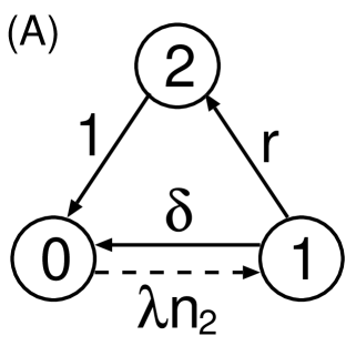
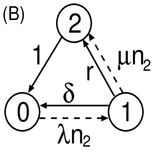
Figure 2: The state-transition rules of (A) the two-stage contact process and (B) the tuberculosis model.

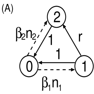
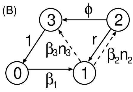
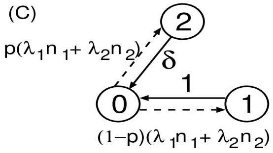
Figure 3: The state-transition rules of the models with competing pathogens analyzed in (A) Sec. III.1, (B) Sec. III.2, and (C) Sec. III.3.

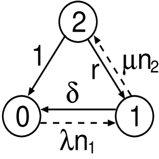
Figure 5: The state-transition rules of the double infection model.

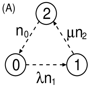
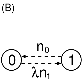
Figure 7: The state-transition rules of (A) the rock-scissors-paper game and (B) the voter model.

In the following, we investigate various contagion models with different transition rules. Because we can never be exhaustive, our strategy is to study known multiple-state models. It will turn out that the extinction of epidemic thresholds as $\left<k^{2}\right>/\left<k\right>$ goes to infinity is not a universal story, as summarized in Sec. VII. What determines the nature of phase boundaries is considered to be the gross organization of the transition pathways, some of which are independent of the state of the neighbors (solid lines in Figs. 1, 2, 3, 5, 7) and others are neighbor-dependent (dashed lines). For the introductory purpose, we analyze in this section two three-state models whose epidemic thresholds are proportional to $\left<k\right>/\left<k^{2}\right>$.

II.1 Two-stage Contact Process

Model

The state-transition rules of the two-stage contact process Krone are schematically shown in Fig. 2(A). It differs from the SIRS model (Fig. 1(C)) in that the transition rate from 0 to 1 is proportional to the density of the neighbors with state 2 (not 1) of a state-0 vertex. This model corresponds to dynamics with two life stages. The states can be interpreted as 0: vacant, 1: occupied by young individuals, and 2: occupied by adults. Only adults are reproductive and generate offsprings in neighboring vacant sites at a birth rate equal to $\lambda$. In other words, a birth event occurs at a vacant site at a rate proportional to $\lambda$ and the number of neighboring adults. Youngs (state 1) spend random time of mean $r$ before becoming adult (state 2). They are also subject to random death events at a rate of $\delta$. Adults die at a rate of 1, which gives normalization of the entire model. Alternatively, we can interpret the three states as 0: vacant, 1: partially occupied, and 2: fully occupied colonies. Then, only fully occupied colonies are potent enough to colonize vacant lands. In the disease analogue, 0 is susceptible, 1 is infected but in the incubation period (not infectious), and 2 is infected and infectious. We note that the model corresponds to the SEIRS model without the recovery state R.

The ordinary contact process (Fig. 1(A)) is recovered as $r=\infty$. In this case, a state-1 vertex immediately turns into state 2. The meanfield approximation and the rigorous results on regular lattices conclude that there are two phases: $\{0\}$ (the steady state that consists only of state 0) and $\{0,1,2\}$ (positive probability of steady coexistence of 0, 1, and 2). Naturally, large $\lambda$ or $r$ promotes survival Krone . Particularly, in the meanfield approximation, these two phases are divided by $r\lambda=\delta+r$.

Analysis

To derive meanfield dynamics for populations with heterogeneous contact rates, let us denote by $p_{k}$ the probability that a vertex has degree $k$. Obviously, $\sum_{k=1}^{\infty}p_{k}=1$. We denote by $\rho_{i,k}$ ($i=1,2$) the probability that a vertex with degree $k$ takes state $i$. The probability that a vertex with degree $k$ takes state 0 is equal to $1-\rho_{1,k}-\rho_{2,k}$. The probability that a neighbor located at the end of a randomly chosen edge takes state $i$ is denoted by $\Theta_{i}$. This edge-conditioned probability, particularly $\Theta_{2}$ in this model, is used to determine the effective infection rate Pastor01PRL ; Pastor01PRE .

The dynamics are given by

$$\dot{\rho}_{1,k} = \lambda(1-\rho_{1,k}-\rho_{2,k})k\Theta_{2}-(\delta+r)\rho_{1,k},$$

$$\dot{\rho}_{2,k} = r\rho_{1,k}-\rho_{2,k}.$$ (1)

We note that the effective birth rate (the first term in the first equation of Eq. (1)) is proportional to $k\Theta_{2}$, which is the average number of state-2 vertices in the neighborhood of a degree-$k$ vertex.

When we choose an arbitrary edge, the probability that a specific vertex is connected to this edge is proportional to its degree $k$ Callaway00 ; Cohen00PRL ; Pastor01PRL ; Pastor01PRE ; Newman02_bond . Therefore, we obtain

$$\Theta_{i}=\frac{\sum_{k}kp_{k}\rho_{i,k}(t)}{\left<k\right>}.$$ (2)

The steady state is given by

$$\rho^{*}_{1,k} = \frac{\rho^{*}_{2,k}}{r},$$

$$\rho^{*}_{2,k} = \frac{\lambda r\Theta^{*}_{2}k}{\delta+r+\lambda(r+1)\Theta^{*}_{2}k},$$ (3)

where $*$ indicates the steady state. Plugging Eq. (3) into Eq. (2) leads to

$$\Theta^{*}_{2}=\frac{1}{\left<k\right>}\sum_{k}\frac{\lambda r\Theta^{*}_{2}k^{2}p_{k}}{\delta+r+\lambda(r+1)\Theta^{*}_{2}k}.$$ (4)

Equation (4) is satisfied when $\Theta^{*}_{2}=0$, corresponding to the disease-free state $\{0\}$. When $0<\Theta^{*}_{2}<1$, state 2 survives. Equation (3) implies $\rho^{*}_{1,k},\rho^{*}_{2,k}>0$ in this situation. Accordingly, $\Theta^{*}_{2}>0$ is equivalent to the $\{0,1,2\}$ phase. Because the RHS of Eq. (4) is smaller than the LHS when $\Theta^{*}_{2}=1$, the condition for the $\{0,1,2\}$ phase is

$$\left.\frac{\partial}{\partial\Theta^{*}_{2}}\left(\frac{1}{\left<k\right>}\sum_{k}\frac{\lambda r\Theta^{*}_{2}k^{2}p_{k}}{\delta+r+\lambda(r+1)\Theta^{*}_{2}k}.\right)\right|_{\Theta^{*}_{2}=0}>1.$$ (5)

This yields

$$\lambda>\frac{(\delta+r)\left<k\right>}{r\left<k^{2}\right>}.$$ (6)

When $p_{k}\propto k^{-\gamma}$ ($\gamma\leq 3$), the critical infection rate vanishes. This agrees with the results for the percolation, the contact process, and the SIR model.

II.2 Tuberculosis Model

Model

A next example is the tuberculosis model shown in Fig. 2(B) Schinazi03_JTB . In the tuberculosis, a majority of the infected individuals does not become infectious before recovery. Accordingly, state 0 corresponds to healthy, 1 to infected but not infectious, and 2 to infected and infectious. This model, which is an extension of the two-stage contact process, has two important features. One is that we have two state-transition routes that depend on neighbors’ states. Both of them depend on the density of infectious individuals (state 2). Antoher feature is that disease progression from state 1 to 2 is possible through two parallel routes. An early-stage patient (state 1) can develop the disease on its own at a rate of $r$. At the same time, infectious patients (state 2) in the neighborhood increases the possibility of disease progression for a state-1 individual.

When $r=0$, the $\{0,1,2\}$ phase is possible on regular lattices but impossible in perfectly mixed populations Schinazi03_JTB . When $r>0$, the $\{0\}$ phase and the $\{0,1,2\}$ phase appear for both lattices and meanfield populations, depending on values of other parameters. According to the ordinary meanfield analysis, these phases are divided by $\lambda r=(\delta+r)$, which is the condition identical to that for the two-stage contact process.

Analysis

In heterogeneous populations, the dynamics become

$$\dot{\rho}_{1,k} = \lambda(1-\rho_{1,k}-\rho_{2,k})k\Theta_{2}-\mu\rho_{1,k}k\Theta_{2}-(\delta+r)\rho_{1,k},$$

$$\dot{\rho}_{2,k} = \mu\rho_{1,k}k\Theta_{2}+r\rho_{1,k}-\rho_{2,k}.$$ (7)

The steady state is given by

$$\left(\begin{array}[]{c}\rho^{*}_{1,k}\\ \rho^{*}_{2,k}\end{array}\right)=\frac{\lambda\Theta^{*}_{2}k}{\delta+r+(\lambda+\mu+\lambda r)\Theta^{*}_{2}k+\lambda\mu\Theta^{*2}_{2}k^{2}}\left(\begin{array}[]{c}1\\ r+\mu k\Theta^{*}_{2}\end{array}\right),$$ (8)

and

$$\Theta^{*}_{2}=\frac{1}{\left<k\right>}\sum_{k}\frac{\lambda k^{2}(r+\mu k\Theta^{*}_{2})\Theta^{*}_{2}p_{k}}{\delta+r+(\lambda+\mu+\lambda r)k\Theta^{*}_{2}+\lambda\mu k^{2}\Theta^{*2}_{2}}.$$ (9)

The $\{0,1,2\}$ phase appears when $\Theta^{*}_{2}>0$, or

$$\lambda>\frac{(\delta+r)\left<k\right>}{r\left<k^{2}\right>}.$$ (10)

This is identical to Eq. (6).

III Models with Competing Pathogens

In many epidemics, multiple strains or pathogens with different transmissivity, virulence, and mobility coexist. They compete with each other by preying on common susceptible individuals. On top of that, transitions between infected states with different pathogens or stages of the disease can occur owing to mutation and disease progression. Coexistence of two distinct diseases in a population also introduces competition between them.

In terms of schematic diagrams, this means that multiple neighbor-dependent infection pathways (dashed lines) emanate from a susceptible state. We analyze three models with competiting pathogens and show that epidemic thresholds are not entirely governed by the degree-dependent factors in two models.

III.1 A Minimal Model with Pathogen Competition and Mutation

Model

Let us consider a minimal model for competing pathogens whose transition rules are shown in Fig. 3(A). State 1 and state 2 correspond to patients infected with strain 1 and strain 2, respectively. The two strains compete with each other by feeding on the common resource, namely, susceptible individuals (state 0), at rates $\beta_{1}$ and $\beta_{2}$. Any patient spontaneously recovers at rate 1. Unidirectional and spontaneous mutations occur (1 $\to$ 2) at rate $r$ Schinazi01_MPRF . As the mutation rate increases, strain 2 becomes more viable than strain 1. In the poupulation ecology context, the three states can be also interpreted as empty (0), species A (1), and species B (2).

Exploiting the fact that the absence of state-1 vertices is equivalent to the contact process, Schinazi showed for regular lattices that there are three phases $\{0\}$, $\{0,2\}$, and $\{0,1,2\}$ separated by nontrivial critical lines Schinazi01_MPRF . Small $r$ and large $\beta_{1}$ support the $\{0,1,2\}$ state. The meanfield analysis predicts that the boundary between $\{0\}$ and $\{0,2\}$ is $\beta_{2}=1$, and $\{0,1,2\}$ appears when both $\beta_{1}>\beta_{2}(r+1)$ and $\beta_{1}>r+1$ are additionally satisfied.

Analysis

For heterogeneous populations, the dynamics are given by

$$\dot{\rho}_{1,k} = \beta_{1}\left(1-\rho_{1,k}-\rho_{2,k}\right)k\Theta_{1}-(r+1)\rho_{1,k},$$

$$\dot{\rho}_{2,k} = \beta_{2}\left(1-\rho_{1,k}-\rho_{2,k}\right)k\Theta_{2}+r\rho_{1,k}-\rho_{2,k}.$$ (11)

The boundary between $\{0\}$ and $\{0,2\}$ is obtained easily. Application of the contact-process result implies that $\{0,2\}$ emerges when

$$\beta_{2}>\frac{\left<k\right>}{\left<k^{2}\right>},$$ (12)

which extends the condition $\beta_{2}>1$ for homogeneous populations.

We next analyze the boundary between $\{0,2\}$ and $\{0,1,2\}$. With the steady state

$$\left(\begin{array}[]{c}\rho^{*}_{1,k}\\ \rho^{*}_{2,k}\end{array}\right)=\frac{k}{r+1+\left(r+1\right)\left(\beta_{2}\Theta^{*}_{2}+\beta_{1}\Theta^{*}_{1}\right)k}\left(\begin{array}[]{c}\beta_{1}\Theta^{*}_{1}\\ \beta_{1}r\Theta^{*}_{1}+\beta_{2}(r+1)\Theta^{*}_{2}\end{array}\right),$$ (13)

we obtain

$$\Theta^{*}_{1}=\frac{\beta_{1}-\beta_{2}(r+1)}{r\beta_{1}}\Theta^{*}_{2}\equiv C_{1}\Theta^{*}_{2},$$ (14)

and

$$\Theta^{*}_{2}=\frac{1}{\left<k\right>\left(r+1\right)}\sum_{k}\frac{\beta_{1}\Theta^{*}_{2}k^{2}p_{k}}{1+\left(\beta_{1}C_{1}+\beta_{2}\right)\Theta^{*}_{2}k}.$$ (15)

In the $\{0,1,2\}$ phase, $\Theta_{1}>0$ and $\Theta_{2}>0$ are simultaneously satisfied. The condition $\Theta^{*}_{2}>0$ is satisfied when

$$\beta_{1}>\frac{(r+1)\left<k\right>}{\left<k^{2}\right>}.$$ (16)

Equation (16) extends one of the conditions for the $\{0,1,2\}$ phase in the homogeneous population: $\beta_{1}>r+1$. Imposing $\Theta^{*}_{1}>0$ leads to $\beta_{1}>\beta_{2}(r+1)$, a condition independent of heterogeneity in contact rates. Because of this condition, $\left<k^{2}\right>\to\infty$ means survival of state 2 but not necessarily survival of state 1. Increasing $\left<k^{2}\right>/\left<k\right>$ makes the survival of state 1 and state 2 more or less equally likely because they feed on the susceptibles in the same manner. Then, the strengths of 1 and 2 must be balanced so that one does not completely devour the other. This constrains the range of the mutation rate in a degree-independent manner.

Figure 4 shows numerically obtained steady densities of state 1 (A) and 2 (B) in networks with 10000 vertices and $\left<k\right>=12$. Initially, each vertex takes one of the three states independently with probability $1/3$. We set $\beta_{1}=0.5$ and $\beta_{2}=0.25$, which predicts the phase boundary: $r=\beta_{1}/\beta_{2}-1=1$.

Scale-free networks with the degree distribution $p_{k}\propto k^{\gamma}$ with $\gamma=2.5$ (thickest solid lines), $\gamma=3.0$ (moderate solid lines), and $\gamma=4.0$ (thinnest solid lines) are produced using a static model Goh01PRL . Even though produced networks can be disconnected in general, more than 95 % of the vertices constitute one component in every run of our simulations. The results for the random graph, whose $p_{k}$ follows the Poisson distribution, are also shown (dashed lines). Regardless of networks, the numerical results support the existence of finite thresholds in terms of $r$. The values of critical $r$ are slightly smaller than $r=1$ but do not vary so much for different $p_{k}$, as our theory predicts.

III.2 Model of Drug-resistant Diseases

Model

In many diseases such as tuberculosis, drug-resistant strains emerge by the mutation of a wild strain Blower . Misuse of antibiotics is a major cause of appearance of such stronger strains. A four-state model shown in Fig. 3(B) represents spreads of a drug-resistant strain Schinazi99_JSP . The states 0, 1, 2, and 3 represent empty, susceptible, infected with the wild strain, and infected with the drug-resistant strain, respectively. The wild strain (state 2) and the drug-resistant strain (state 3) compete with each other to devour the susceptible (state 1). Only the drug-resistant strain is supposed to be fatal with death rate 1. When infected by the wild strain, which is not lethal, an individual recovers at rate $r$ owing to the drug. The mutation rate is denoted by $\phi$.

The model without state 2 (or $\beta_{2}=0$) is equivalent to the SIRS model in Fig. 1(C) with $\delta=0$. On regular lattices, $\{0,1,2,3\}$ appears when $r+\phi$ is small enough. Otherwise, state 2 is extinguished Schinazi99_JSP . Based on the meanfield analysis, the $\{0,1,2,3\}$ phase ensues when

$$\phi>0,\quad\beta_{2}>r+\phi,\quad\frac{\beta_{2}}{r+\phi}>\beta_{3}.$$ (17)

If any of the conditions in Eq. (17) is violated and $\beta_{3}>1$, then we have $\{0,1,3\}$. Otherwise, only state 1 survives (the $\{1\}$ phase).

Analysis

In heterogeneous populations, we obtain

$$\dot{\rho}_{1,k} = \beta_{1}\left(1-\rho_{1,k}-\rho_{2,k}-\rho_{3,k}\right)+r\rho_{2,k}-\beta_{2}\rho_{1,k}k\Theta_{2}-\beta_{3}\rho_{1,k}k\Theta_{3},$$

$$\dot{\rho}_{2,k} = \beta_{2}\rho_{1,k}k\Theta_{2}-(r+\phi)\rho_{2,k},$$

$$\dot{\rho}_{3,k} = \beta_{3}\rho_{1,k}k\Theta_{3}+\phi\rho_{2,k}-\rho_{3,k}.$$ (18)

The steady densities are given by

$$\left(\begin{array}[]{c}\rho^{*}_{1,k}\\ \rho^{*}_{2,k}\\ \rho^{*}_{3,k}\end{array}\right)=\frac{\beta_{1}}{\Delta}\left(\begin{array}[]{c}r+\phi\\ \beta_{2}\Theta^{*}_{2}k\\ \left[\beta_{2}\phi\Theta^{*}_{2}+\beta_{3}\left(r+\phi\right)\Theta^{*}_{3}\right]k\end{array}\right),$$ (19)

where

$$\Delta\equiv\beta_{1}(r+\phi)+\left[\left(\beta_{1}+\phi+\beta_{1}\phi\right)\beta_{2}\Theta^{*}_{2}+\left(\beta_{1}+1\right)\beta_{3}\left(r+\phi\right)\Theta^{*}_{3}\right]k.$$ (20)

Equation (19) assures that $\rho^{*}_{1,k}>0$. In addition,

$$\Theta^{*}_{3}=\frac{\beta_{2}\phi}{\beta_{2}-\beta_{3}(r+\phi)}\Theta^{*}_{2}$$ (21)

provided that $\beta_{2}\big{/}(r+\phi)>\beta_{3}$. Under this condition, $\Theta^{*}_{2}>0$ is equivalent to the $\{0,1,2,3\}$ phase. Combining Eqs. (2), (19) and (21) results in

$$\Theta^{*}_{2}=\frac{1}{\left<k\right>}\sum_{k}\frac{\beta_{2}\Theta^{*}_{2}k^{2}p_{k}}{\Delta}.$$ (22)

Since $\Delta$ is of the form: $\Delta=C_{3}+C_{4}k\Theta^{*}_{2}$, Eq. (22) is essentially the same as Eq. (4). Accordingly, $\Theta^{*}_{2}>0$ when

$$\beta_{2}>\frac{\beta_{1}(r+\phi)\left<k\right>}{\left<k^{2}\right>}.$$ (23)

Even for large $r+\phi$, sufficiently heterogeneous $p_{k}$ with large $\left<k^{2}\right>\big{/}\left<k\right>$ makes Eq. (23) valid. However, for existence of state 2, $\beta_{2}(r+\phi)>\beta_{3}$ must be also satisfied. This condition is independent of the degree distribution and identical to one of the conditions for the $\{0,1,2,3\}$ phase in the ordinary meanfield case (see Eq. (17)). As is the case for the previous model (Sec. III.1), this condition regulates the rates of mutation and spontaneous recovery so that the strengths of the wild strain and the drug-resistant strain are roughly balanced.

If $\beta_{2}\big{/}(r+\phi)\leq\beta_{3}$, then $\Theta^{*}_{2}=0$. In this case, Eq. (19) reduces to

$$\left(\begin{array}[]{c}\rho^{*}_{1,k}\\ \rho^{*}_{3,k}\end{array}\right)=\frac{\beta_{1}}{\beta_{1}+(\beta_{1}+1)\beta_{3}\Theta^{*}_{3}k}\left(\begin{array}[]{c}1\\ \beta_{3}\Theta^{*}_{3}k\end{array}\right),$$ (24)

which yields

$$\Theta^{*}_{3}=\frac{1}{\left<k\right>}\sum_{k}\frac{\beta_{1}\beta_{3}\Theta^{*}_{3}k^{2}p_{k}}{\beta_{1}+(\beta_{1}+1)\beta_{3}\Theta^{*}_{3}k}.$$ (25)

As a result, $\{0,1,3\}$ and $\{1\}$ are separated by

$$\beta_{3}=\frac{\left<k\right>}{\left<k^{2}\right>}.$$ (26)

In summary, the $\{0,1,2,3\}$ phase dominates even for infinitesimally small infection rates when $\left<k^{2}\right>=\infty$ and $\beta_{2}/(r+\phi)>\beta_{3}$. When the latter condition is violated, $\{0,1,3\}$ appears for a tiny infection rate.

III.3 Superspreader Model

Model

Superspreaders, namely, patients that infect many others in comparison with normal patients, are identified in the outbreaks in, for example, gonorrhea Hethcote84 , HIV Anderson86 ; May88TRANS ; Colgate , and SARS, Abdullah ; Singapore . Such heterogeneous infection rates are sometimes ascribed to heterogeneous social or sexual contact rates as specified by $p_{k}$ Hethcote84 ; Anderson86 ; May88TRANS ; Liljeros ; Meyers03 ; Schneeberger . However, superspreaders exist even in diseases whose associated networks are considered to have relatively homogeneous $k$, such as SARS Masuda_SARS . Then, an alternative way to introduce superspreaders is to consider two types of patients with different infection rates. Then, competition occurs between superspreaders and normal patients.

We assume that superspreaders and normally infectious patients are not distinguished by the strain types. Accordingly, an infection event originating from a superspreader can cause a normal patient and vice versa. There is no mutation, and competition occurs indirectly. That is how the superspreader model considered here is essentially different from the models in Secs. III.1 and III.2.

We analyze a three-state model with different infection rates, which is schematically shown in Fig. 3(C) Kemper78 ; Schinazi01_MB . The states 0, 1, and 2 mean susceptible, patients of type 1 with infection rate $\lambda_{1}$ and recovery rate 1, and patients of type 2 with infection rate $\lambda_{2}\geq\lambda_{1}$ and recovery rate $\delta$, respectively. State 2 corresponds to the superspreader, and in practical appliations, we put $\lambda_{1}\ll\lambda_{2}$. Upon infection, a state-0 vertex changes its state into 1 (2) with probability $1-p$ ($p$). There are two neighbor-dependent infection routes in Fig. 3(C). State 1 and state 2 indirectly compete with each other through crosstalk. In other words, the density of state 1 and that of state 2 affect the rates of transitions $0\to 2$ and $0\to 1$, respectively. According to the meanfield analysis, $\{0,1,2\}$ results when

$$\lambda_{1}\delta(1-p)+\lambda_{2}p>\delta.$$ (27)

Otherwise, $\{0\}$ results. Slightly weaker but qualitatively similar results have been proved for lattices Schinazi01_MB .

Analysis

In heterogeneous populations, dynamics are given by

$$\dot{\rho}_{1,k} = (1-p)\left(1-\rho_{1,k}-\rho_{2,k}\right)k(\lambda_{1}\Theta_{1}+\lambda_{2}\Theta_{2})-\rho_{1,k},$$

$$\dot{\rho}_{2,k} = p\left(1-\rho_{1,k}-\rho_{2,k}\right)k(\lambda_{1}\Theta_{1}+\lambda_{2}\Theta_{2})-\delta\rho_{2,k}.$$ (28)

The steady state is:

$$\left(\begin{array}[]{c}\rho^{*}_{1,k}\\ \rho^{*}_{2,k}\end{array}\right)=\frac{(\lambda_{1}\Theta^{*}_{1}+\lambda_{2}\Theta^{*}_{2})k}{\delta+\left[p+\delta\left(1-p\right)\right](\lambda_{1}\Theta^{*}_{1}+\lambda_{2}\Theta^{*}_{2})k}\left(\begin{array}[]{c}\delta(1-p)\\ p\end{array}\right),$$ (29)

which leads to

$$\Theta^{*}_{1}=\frac{\delta(1-p)}{p}\Theta^{*}_{2}.$$ (30)

Therefore, $\Theta^{*}_{1}>0$, or equivalently, $\overline{\Theta}^{*}\equiv\lambda_{1}\Theta^{*}_{1}+\lambda_{2}\Theta^{*}_{2}>0$, is the condition for the $\{0,1,2\}$ phase. With Eq. (29), we obtain

$$\overline{\Theta}^{*}=\frac{1}{\left<k\right>}\sum_{k}\frac{\left[\lambda_{1}\delta\left(1-p\right)+\lambda_{2}p\right]\overline{\Theta}^{*}k^{2}p_{k}}{\delta+\left[p+\delta\left(1-p\right)\right]k\overline{\Theta}^{*}},$$ (31)

and $\{0,1,2\}$ emerges when

$$\lambda_{1}\delta(1-p)+\lambda_{2}p>\frac{\delta\left<k\right>}{\left<k^{2}\right>}.$$ (32)

Equation (32) suggests that an arbitrary small infection rate $\lambda_{1}$ or $\lambda_{2}$ allows the endemic state as $\left<k^{2}\right>/\left<k\right>\to\infty$. In contrast to the models in Secs. III.1 and III.2, degree-independent factor does not play a role in this model. This is due to the absence of mutation from 1 to 2 or from 2 to 1.

IV Double Infection Model

Model

For a realistic network model of populations with natural birth, we have to take into account that birth can occur only at empty sites. Then, a minimal model such as the contact process must be extended to a three-state process in which states 0, 1, and 2 mean empty, susceptible, and infected, respectively. A susceptible gives birth to an offspring in a neighboring empty vertex, which is operationally similar to a contagion event. An infected preys on a susceptible in its neighborhood. Then there are two neighbor-dependent transition rates, namely, 0 $\to$ 1 transition at a rate proportional to $n_{1}$ and 1 $\to$ 2 transition at a rate proportional to $n_{2}$. A similar situation arises in the context of double infection in which states 0, 1, and 2 correspond to susceptible, infected, and infected by another pathogen, respectively. A second pathogen (state 2) targets individuals infected by a first pathogen (state 1).

Keeping these interpretations in mind, we analyze the model shown in Fig. 5 Sato94 ; Haraguchi . State 2 may more virulent than state 1, and evolution of strains has been investigated with a more complicated version of this model Haraguchi . The model extends the contact process and the SIR model, which correspond to $\mu=0$ and $\lambda=\delta=r=0$, respectively.

This model is theoretically intricate. A subtlety stems from the cascaded neighbor-dependent transitions 0 $\to$ 1 and 1 $\to$ 2 DurrettNeuhauser91 ; Andjel . There are three basic phases $\{0\}$, $\{0,1\}$, and $\{0,1,2\}$. The meanfield solution predicts that $\{0\}$ and $\{0,1\}$ are divided by $\lambda=\delta$. The one-dimensional lattice with $r=0$ does not permit $\{0,1,2\}$ Sato94 ; Andjel . However, on regular lattices of any dimension, introduction of a small recovery rate $r>0$ elicits $\{0,1,2\}$ KST04 . It is counterintuitive in the sense that $r$ is the rate at which state 2 turns into state 1. Indeed, the meanfield theory predicts the $\{0,1,2\}$ phase for sufficiently small $r$ fulfilling

$$\frac{\delta}{\lambda}+\frac{r+1}{\mu}<1.$$ (33)

Another paradoxical behavior occurs regarding to population density. For example, an increase in $\lambda$ lessens the number of state-1 vertices on lattices because a larger $\lambda$ creates more preys to devour for state-2 vertices Tainaka03 . Similarly, too large $\mu$ drives state 2 to perish due to excess mortality Sato94 ; Haraguchi , which defines another $\{0,1\}$ phase that we do not examine here. This $\{0,1\}$ phase is distinct from the $\{0,1\}$ phase revealed by the meanfield equations and mathematical analysis on lattices.

This model is complex also in the sense that the phase diagram in the parameter space is even qualitatively unknown for lattices. The meanfield solution indicates that the two critical lines approach each other as $\mu\to\infty$. On the other hand, they may cross at finite $\lambda$ and $\mu$, as supported by the improved pair approximation ansatz Sato94 ; Haraguchi .

Analysis

In heterogeneous populations, the dynamics read

$$\dot{\rho}_{1,k} = \lambda(1-\rho_{1,k}-\rho_{2,k})k\Theta_{1}-\delta\rho_{1,k}+r\rho_{2,k}-\mu\rho_{1,k}k\Theta_{2},$$

$$\dot{\rho}_{2,k} = \mu\rho_{1,k}k\Theta_{2}-(r+1)\rho_{2,k}.$$ (34)

The steady state is given by

$$\left(\begin{array}[]{c}\rho^{*}_{1,k}\\ \rho^{*}_{2,k}\end{array}\right)=\frac{\lambda\Theta^{*}_{1}k}{\delta(r+1)+\left[\lambda(r+1)\Theta^{*}_{1}+\mu\Theta^{*}_{2}\right]k+\lambda\mu\Theta^{*}_{1}\Theta^{*}_{2}k^{2}}\left(\begin{array}[]{c}r+1\\ \mu\Theta^{*}_{2}k\end{array}\right),$$ (35)

which leads to

$$\left(\begin{array}[]{c}\Theta^{*}_{1}\\ \Theta^{*}_{2}\end{array}\right)=\frac{1}{\left<k\right>}\sum_{k}\frac{\lambda\Theta^{*}_{1}k^{2}p_{k}}{\delta(r+1)+\left[\lambda(r+1)\Theta^{*}_{1}+\mu\Theta^{*}_{2}\right]k+\lambda\mu\Theta^{*}_{1}\Theta^{*}_{2}k^{2}}\left(\begin{array}[]{c}r+1\\ \mu\Theta^{*}_{2}k\end{array}\right).$$ (36)

Clearly, $(\Theta^{*}_{1},\Theta^{*}_{2})=(0,0)$, which corresponds to the $\{0\}$ phase, solves Eq. (36). To explore other phases, let us set

$$f_{1}(\Theta^{*}_{1},\Theta^{*}_{2})\equiv\frac{\lambda(r+1)}{\left<k\right>}\sum_{k}\frac{k^{2}p_{k}}{\delta(r+1)+\left[\lambda(r+1)\Theta^{*}_{1}+\mu\Theta^{*}_{2}\right]k+\lambda\mu\Theta^{*}_{1}\Theta^{*}_{2}k^{2}}-1,$$ (37)

and

$$f_{2}(\Theta^{*}_{1},\Theta^{*}_{2})\equiv\frac{\lambda\mu\Theta^{*}_{1}}{\left<k\right>}\sum_{k}\frac{k^{3}p_{k}}{\delta(r+1)+\left[\lambda(r+1)\Theta^{*}_{1}+\mu\Theta^{*}_{2}\right]k+\lambda\mu\Theta^{*}_{1}\Theta^{*}_{2}k^{2}}-1.$$ (38)

Then Eq. (36) is equivalent to $\Theta^{*}_{1}f_{1}(\Theta^{*}_{1},\Theta^{*}_{2})=0$ and $\Theta^{*}_{2}f_{2}(\Theta^{*}_{1},\Theta^{*}_{2})=0$.

First, we identify the boundary between $\{0\}$ and $\{0,1\}$. In the $\{0,1\}$ phase, we have $\Theta^{*}_{2}=0$. Under this condition, we look for $0<\Theta^{*}_{1}<1$ that satisfies $f_{1}(\Theta^{*}_{1},0)=0$. By substituting $\Theta^{*}_{2}=0$ into Eq. (37), we obtain

$$f_{1}(\Theta^{*}_{1},0)=\frac{\lambda}{\left<k\right>}\sum_{k}\frac{k^{2}p_{k}}{\delta+\lambda\Theta^{*}_{1}k}-1=0.$$ (39)

Because

$$f_{1}(1,0)=\frac{\lambda}{\left<k\right>}\sum_{k}\frac{k^{2}p_{k}}{\delta+\lambda k}-1\leq\frac{\lambda}{\left<k\right>}\sum_{k}\frac{k^{2}p_{k}}{\lambda k}-1\leq 0,$$ (40)

Eq. (39) is satisfied when $f_{1}(0,0)>0$, that is,

$$\frac{\lambda}{\delta}>\frac{\left<k\right>}{\left<k^{2}\right>}.$$ (41)

This conclusion complies with the results for the contact process (Sec. I).

Second, we examine the boundary between $\{0,1\}$ and $\{0,1,2\}$. The $\{0,1,2\}$ phase implies $\Theta^{*}_{1}>0$ and $\Theta^{*}_{2}>0$ such that $f_{1}(\Theta^{*}_{1},\Theta^{*}_{2})=0$ and $f_{2}(\Theta^{*}_{1},\Theta^{*}_{2})=0$. Let us suppose that Eq. (41) is satisfied because $\{0\}$ results otherwise. Then, there is a $0<\overline{\Theta}_{1}\leq 1$ that satisfies Eq. (39). Since $\partial f_{1}/\partial\Theta^{*}_{1}<0$ and $\partial f_{1}/\partial\Theta^{*}_{2}<0$, there is a curve $f_{1}(\Theta^{*}_{1},\Theta^{*}_{2})=0$ in the $\Theta^{*}_{1}$-$\Theta^{*}_{2}$ space that looks like the solid line (I) (when $f_{1}(0,1)\leq 0$), or (II) (when $f_{1}(0,1)>0$) in Fig. 6(A).

Because $\partial f_{2}/\Theta^{*}_{1}>0$ and $\partial f_{2}/\partial\Theta^{*}_{2}<0$, $f_{2}$ monotonically increases in $\Theta^{*}_{1}$ on lines $\Theta^{*}_{2}=0$ and $\Theta^{*}_{1}+\Theta^{*}_{2}=1$. If the isocline $f_{2}(\Theta^{*}_{1},\Theta^{*}_{2})=0$ is located as the dashed line in Fig. 6(B), it nontrivially crosses $f_{1}(\Theta^{*}_{1},\Theta^{*}_{2})=0$ (one of the solid lines) to yield the $\{0,1,2\}$ phase. Because $f_{2}(0,\Theta^{*}_{2})=-1$ ($0\leq\Theta^{*}_{2}\leq 1$), $f_{2}(1,0)>0$ is necessary for the dashed line to exist. Then, there is a unique $0<\overline{\Theta}<1$ so that $f_{2}(\overline{\Theta},1-\overline{\Theta})=0$. Finally, $f_{1}(\Theta^{*}_{1},\Theta^{*}_{2})=0$ and $f_{2}(\Theta^{*}_{1},\Theta^{*}_{2})=0$ cross when (i) $f_{2}(\overline{\Theta}_{1},0)>0$ and (ii) $f_{1}(\overline{\Theta},1-\overline{\Theta})<0$ are both satisfied. Using

$$f_{1}(\overline{\Theta}_{1},0)=\frac{\lambda}{\left<k\right>}\sum_{k}\frac{k^{2}p_{k}}{\delta+\lambda\overline{\Theta}_{1}k}-1=0,$$ (42)

the condition (i) is equivalent to

$$f_{2}(\overline{\Theta}_{1},0) = \frac{\lambda\mu\overline{\Theta}_{1}}{(r+1)\left<k\right>}\sum_{k}\frac{k^{3}p_{k}}{\delta+\lambda\overline{\Theta}_{1}k}-1$$ (43)

$$= \frac{\lambda\mu\overline{\Theta}_{1}}{(r+1)\left<k\right>}\sum_{k}\frac{k^{3}p_{k}}{\delta+\lambda\overline{\Theta}_{1}k}-1+\frac{\mu\delta}{(r+1)\lambda}f_{1}(\overline{\Theta}_{1},0)$$

$$= \frac{\mu\left<k^{2}\right>}{(r+1)\left<k\right>}-\left(1+\frac{\mu\delta}{(r+1)\lambda}\right)>0,$$

that is,

$$\frac{\delta}{\lambda}+\frac{r+1}{\mu}<\frac{\left<k^{2}\right>}{\left<k\right>},$$ (44)

which is an extension of the ordinary meanfield solution (Eq. (33)). We note that (i) implies $f_{2}(1,0)>0$, which we required beforehand.

To show (ii), define

$$C_{5}\equiv\frac{\lambda(r+1)(1-\overline{\Theta})}{\lambda(r+1)\overline{\Theta}+\mu(1-\overline{\Theta})}.$$ (45)

We obtain

$$f_{1}(\overline{\Theta},1-\overline{\Theta})$$ (46)

$$= f_{1}(\overline{\Theta},1-\overline{\Theta})+C_{5}f_{2}\left(\overline{\Theta},1-\overline{\Theta}\right)$$

$$= \frac{\lambda}{\left<k\right>}\sum_{k}\frac{(r+1+C_{5}\mu\overline{\Theta}k)k^{2}p_{k}}{\delta(r+1)+\left[\lambda(r+1)\overline{\Theta}+\mu\left(1-\overline{\Theta}\right)\right]k+\lambda\mu\overline{\Theta}\left(1-\overline{\Theta}\right)k^{2}}-1-C_{5}$$

$$< \frac{\lambda}{\left<k\right>}\sum_{k}\frac{(r+1+C_{5}\mu\overline{\Theta}k)k^{2}p_{k}}{\left[\lambda(r+1)\overline{\Theta}+\mu\left(1-\overline{\Theta}\right)\right]k+\lambda\mu\overline{\Theta}\left(1-\overline{\Theta}\right)k^{2}}-1-C_{5}$$

$$= -\frac{\mu(1-\overline{\Theta})}{\lambda(r+1)\overline{\Theta}+\mu(1-\overline{\Theta})}\leq 0.$$

To summarize, both $\{0\}$ and $\{0,1\}$ disappear to be replaced by $\{0,1,2\}$ as $\left<k^{2}\right>\to\infty$.

V Rock-Scissors-Paper Game

Model

Winnerless cyclic competition among different phenotypes abounds in nature. For example, real microbial communities of Escherichia coli Kerr02 ; Kirkup04 and color polymorphisms of natural lizards Sinervo96 have cyclically dominating three states. The evolutionary public-good game with volunteering (choice of not joining the game) also defines a three-state population dynamics with cyclic competition Szabo02 ; Semmann03 . A typical consequence of these dynamics is oscillatory population density with each phenotype alternatively dominant.

Let us consider a simple rock-scissors-paper game with cyclic competition (Fig. 7(A)). The ordinary meanfield analysis yields a single phase: a neutrally stable periodic orbit in which the densities of states 0, 1, and 2 are cyclically dominant Hopbauerbook . The coexistence equilibrium inside the limit cycle is stabilized on regular lattices Tainaka94 ; Frean01 and trees Sato97 . Consequently, convergence to $\{0,1,2\}$ with a damped oscillation occurs on these graphs. We focus on the steady states only in the following analysis.

Analysis

The dynamics in heterogeneous populations are given by

$$\dot{\rho}_{1,k} = \lambda(1-\rho_{1,k}-\rho_{2,k})k\Theta_{1}-\mu\rho_{1,k}k\Theta_{2},$$

$$\dot{\rho}_{2,k} = \mu\rho_{1,k}k\Theta_{2}-\rho_{2,k}k(1-\Theta_{1}-\Theta_{2}),$$ (47)

which yields

$$\left(\begin{array}[]{c}\rho^{*}_{1,k}\\ \rho^{*}_{2,k}\end{array}\right)=\frac{\lambda\Theta^{*}_{1}}{(\lambda\Theta^{*}_{1}+\mu\Theta^{*}_{2})(1-\Theta^{*}_{1}-\Theta^{*}_{2})+\lambda\mu\Theta^{*}_{1}\Theta^{*}_{2}}\left(\begin{array}[]{c}1-\Theta^{*}_{1}-\Theta^{*}_{2}\\ \mu\Theta^{*}_{2}\end{array}\right).$$ (48)

Noting that Eq. (48) is independent of $k$, we obtain

$$\left(\begin{array}[]{c}\Theta^{*}_{1}\\ \Theta^{*}_{2}\end{array}\right)=\left(\begin{array}[]{c}\rho^{*}_{1,k}\\ \rho^{*}_{2,k}\end{array}\right)=\frac{1}{\lambda+\mu+1}\left(\begin{array}[]{c}1\\ \lambda\end{array}\right),$$ (49)

for any $k$. The degree distribution does not affect the steady state.

Similarly, it is straightforward to show that degree distributions are irrelevant in the voter model (Fig. 7(B)) and cyclic interaction models with more than three states Sato02 ; Szabo04PRE . A lesson from these examples is that heterogeneous contact rates do not influence the equilibrium population density if there is no neighbor-independent state transition. However, models with at least one neighbor-independent transitions show extinction of the epidemic threshold as $\left<k^{2}\right>/\left<k\right>\to\infty$. For example, variants of the rock-scissors-paper game supplied with spontaneous death or mutation rates Tainaka03 are expected to belong to the class analyzed in Sec. IV.

VI Two-population Model

Model

In many infectious diseases of humans, such as malaria, yellow feber, and dengue feber, transmission are mediated by other hosts such as mosquitoes. In these diseases, direct human-human or mosquito-mosquito infection is absent, and two distinct populations transmit diseases between each other. As an example, we analyze a model for malaria spreads (Anderson and May, 1991, Ch. 14). Following the original notation, the meanfield dynamics are represented by

$$\dot{y} = \frac{ab\Omega}{N}(1-y)\psi-\gamma y,$$

$$\dot{\psi} = acy(1-\psi)-\mu\psi,$$ (50)

where $y$ and $\psi$ are the proportions of infected humans and mosquitoes, respectively. The size of the human population is denoted by $N$, and $\Omega$ is the size of the female mosquito population; only female mosquitoes infect humans. In addition, $a$ is the bite rate, $b$ and $c$ are infection rates, $\gamma$ is the recovery rate of the humans, and $\mu$ is the death rate of the mosquitoes. Infected humans and infected mosquitoes survive simultaneously if they do. Based on Eq. (50), this occurs when

$$R_{0}\equiv\frac{a^{2}bc\Omega}{N\gamma\mu}>1.$$ (51)

Otherwise, the malaria is eradicated.

Analysis

How does this condition change by introducing heterogeneous contact rates? In network terminology, relevant networks are bipartite, with each part representing the human population and the mosquito population. Let us denote the degree distributions of humans and mosquitoes by $\{p_{y,k}\}$ and $\{p_{\psi,k}\}$, respectively. Real data do not suggest that $\{p_{y,k}\}$ or $\{p_{\psi,k}\}$ is scale-free. However, we treat general degree distributions because the obtained results may apply to other multi-population contagion processes.

The dynamics are given by

$$\dot{y}_{k} = \frac{ab\Omega}{N}(1-y_{k})k\Theta_{\psi}-\gamma y_{k},$$

$$\dot{\psi}_{k} = ac(1-\psi_{k})k\Theta_{y}-\mu\psi_{k},$$ (52)

where $y_{k}$ ($\psi_{k}$) is the probability that humans (mosquitoes) with degree $k$ are infected, and

$$\Theta_{y} \equiv \frac{1}{\left<k\right>_{y}}\sum_{k}kp_{y,k}y_{k},\quad\left<k\right>_{y}\equiv\sum_{k}kp_{y,k},$$

$$\Theta_{\psi} \equiv \frac{1}{\left<k\right>_{\psi}}\sum_{k}kp_{\psi,k}\psi_{k},\quad\left<k\right>_{\psi}\equiv\sum_{k}kp_{\psi,k}.$$ (53)

The steady state is calculated as

$$\left(y^{*}_{k},\psi^{*}_{k}\right)=\left(\frac{ab\Omega\Theta^{*}_{\psi}k}{N\gamma+ab\Omega\Theta^{*}_{\psi}k},\frac{ac\Theta^{*}_{y}k}{\mu+ac\Theta^{*}_{y}k}\right),$$ (54)

which is solved trivially by $(\Theta^{*}_{y},\Theta^{*}_{\psi})=(0,0)$. To explore nontrivial solutions, let us eliminate $\Theta^{*}_{\psi}$ from Eqs. (53) and (54) to obtain

$$\Theta^{*}_{y}=\frac{1}{\left<k\right>_{y}}\sum_{k}\frac{ab\Omega k^{2}p_{y,k}\sum_{k^{\prime}}\frac{ac\Theta^{*}_{y}k^{\prime 2}p_{\psi,k^{\prime}}}{\mu+ac\Theta^{*}_{y}k^{\prime}}}{N\gamma\left<k\right>_{\psi}+ab\Omega kp_{y,k}\sum_{k^{\prime}}\frac{ac\Theta^{*}_{y}k^{\prime 2}p_{\psi,k^{\prime}}}{\mu+ac\Theta^{*}_{y}k^{\prime}}}.$$ (55)

The RHS of Eq. (55) is less than 1 when $\Theta^{*}_{y}=1$. The endemic state results if

$$\frac{\partial}{\partial\Theta^{*}_{y}}\left(\mbox{RHS of Eq.~{}(\ref{eq:malaria_d})}\right)\bigg{|}_{\Theta^{*}_{y}=0}=\frac{a^{2}bc\Omega\left<k^{2}\right>_{y}\left<k^{2}\right>_{\psi}}{N\gamma\mu\left<k\right>_{y}\left<k\right>_{\psi}}>1,$$ (56)

which extends Eq. (51). Equation (56) indicates that divergence of just either $\left<k^{2}\right>_{y}$ or $\left<k^{2}\right>_{\psi}$ is sufficient for the epidemic threshold to disappear. Even if both moments are finite, their effects are multiplicative. This is consistent with the results for two-sex models of heterosexual HIV transmissions May88TRANS and the bond percolation on bipartite graphs Newman02_bond ; Meyers03 .

VII Conclusions

We have analyzed various models of endemic infectious diseases in populations with heterogeneous contact rates, or on complex networks. The effects of heterogeneity on epidemic thresholds are summarized in Tab. 1. In many models, diverging second moments of the degree distribution extinguishes the epidemic thresholds, as reported previously for the percolation Albert00NAT ; Callaway00 ; Cohen00PRL ; Newman02_bond , the contact process Hethcote84 ; Pastor01PRL ; Pastor01PRE , the SIR model Anderson86 ; May88TRANS ; May01 ; Moreno02EPB , the SIRS model Liu04JSM , and the household moodel Liu04PHA . On scale-free networks, which underly sexually transmitted diseases and computer viruses (see Sec. I for references), introduction of a tiny amount of virus to a population can cause an endemic state even in models with more complex transition rules.

However, the models with competing pathogens and mutation (Secs. III.1 and III.2) show different behavior. The heterogeneity in contact rates equally boosts the infection strengths of competing pathogens in these models. Whether multiple strains survive or one overwhelms the others depends on network-independent mutation rates that modulate relative strengths of pathogens. The rock-scissors-paper game and the voter model stipulate another class of models in which heterogeneity does not affect the equilibrium population density at all. For the heterogeneity to take effects, there must be at least one neighbor-independent transition rate.

For a fixed graph or a contact rate distribution, one can create new models that are not convered by this paper. Our analysis has not been exhaustive. However, we consider that what essentially matters is gross arrangements of contagion pathways. If there is at least one transmission route independent of the neighbors’ states, which is not the case for the rock-srissors-paper game, the equilibrium population density will depend on degree distributions as does the contact process. A care must be paid to cases of competing pathogens with mutation. We hope that our results give prescription for understanding complex-network consequences of other models.

A last note is on the stability of solutions. For the contact process on complex networks, the coexistence phase is stable if it exists Andersonbook ; Olinsky . Similarly, the stability of the simplest nontrivial phase is assured for models analyzed in this paper. However, stability analysis of other phases seems mathematically difficult. In addition, the stability of coexistence solutions of the rock-scissors-paper game shows network dependence Masuda06RSP . These topics are warranted for future work.

Figure 4: Numerically obtained stationary densities of (A) state 1 and (B) state 2 for the model in Sec. III.1 (see Fig. 3(A) for the transition rules). The scale-free networks with $\gamma=2.5$ (thickest solid lines), $\gamma=3.0$ (moderate solid lines), $\gamma=4.0$ (thinnest solid lines), and the random graph (dotted lines) are used. See the text for other parameter values.

Figure 6: (A) The isocline $f_{1}=0$ (solid lines) and sign of $f_{1}$, (B) $f_{2}=0$ (dashed line) and sign of $f_{2}$ superimposed on $f_{1}=0$ (solid lines).

Table 1: Summary of the effects of heterogeneous contact rates on epidemic thresholds.

model	phases	threshold $\to 0$	remarks	section
		as $\left<k^{2}\right>\to\infty$
CP	$\{0\}$, $\{0,1\}$	yes	similar for SIR,	I
			SIRS, household
two-stage CP	$\{0\}$, $\{0,1,2\}$	yes		II.1
tuberculosis	$\{0\}$, $\{0,1,2\}$	yes		II.2
2 pathogens	$\{0\}$, $\{0,2\}$,	yes	$\{0,1,2\}$ requires a	III.1
with mutation	$\{0,1,2\}$		$p_{k}$-indep. condition
drug-resistant	$\{1\}$, $\{0,1,3\}$,	yes	$\{0,1,2,3\}$ requires a	III.2
	$\{0,1,2,3\}$		$p_{k}$-indep. condition
superspreader	$\{0\}$, $\{0,1,2\}$	yes		III.3
double infection	$\{0\}$, $\{0,1\}$, $\{0,1,2\}$	yes for both		IV
		$\{0\}$ and $\{0,1\}$
rock-scissors-paper	$\{0,1,2\}$	no	similar for	V
			the voter model
malaria	nonendemic, endemic	yes		VI

References

- (1) Abdullah, A.S.M., Tomlinson, B., Cockram, C.S., Thomas, G.N., 2003. Lessons from severe acute respiratory syndrome outbreak in Hong Kong. Emerg. Infect. Dis. 9(9), 1042–1045.
- (2) Albert, R., Jeong, H., Barabási, A.-L., 2000. Error and attack tolerance of complex networks. Nature 406, 378–382.
- (3) Albert, R., Barabási, A.-L., 2002. Statistical mechanics of complex networks. Rev. Mod. Phys. 74, 47–97.
- (4) Anderson, R.M., Medley, G.F., May, R.M., Johnson, A.M., 1986. A preliminary study of the transmission dynamics of the human immunodeficiency virus (HIV), the causative agent of AIDS. IMA J. Math. Appl. Med. Biol. 3, 229–263.
- (5) Anderson, R.M., May, R.M., 1991. “Infectious diseases of humans,” Oxford University Press, Oxford.
- (6) Andjel, E., Schinazi, R., 1996. A complete convergence theorem for an epidemic model. J. Appl. Prob. 33, 741–748.
- (7) Barabási, A.-L., and Albert, R., 1999. Emergence of scaling in random networks. Science 286, 509–512.
- (8) Blower, S.M., Small, P.M., Hopewell, P.C., 1996. Control strategies for tuberculosis epidemics: new models for old problems. Science 273, 497–500.
- (9) Callaway, D.S., Newman, M.E.J., Strogatz, S.H., Watts, D.J., 2000. Network robustness and fragility: percolation on random graphs. Phys. Rev. Lett. 85, 5468–5471.
- (10) Cohen, R., Erez, K., ben-Avraham, D., Havlin, S., 2000. Resilience of the Internet to random breakdowns. Phys. Rev. Lett. 85, 4626–4628.
- (11) Colgate, S.A., Stanley, E.A., Hyman, J.M., Layne, S.P., Qualls, C., 1989. Risk behavior-based model of the cubic growth of acquired immunodeficiency syndrome in the United States. Proc. Natl. Acad. Sci. U.S.A. 86, 4793–4797.
- (12) Durrett, R., Neuhauser, C., 1991. Epidemics with recovery in . Ann. Appl. Prob. 1(2), 189–206.
- (13) Frean, M., Abraham, E.R., 2001. Rock-scissors-paper and the survival of the weakest. Proc. R. Soc. London B 268, 1323–1327.
- (14) Goh, K.-I., Kahng, B., Kim, D., 2001. Universal behavior of load distribution in scale-free networks. Phys. Rev. Lett. 87, 278701.
- (15) Haraguchi, Y., Sasaki, A., 2000. The evolution of parasite virulence and transmission rate in a spatially structured population. J. Theor. Biol. 203, 85–96.
- (16) Hethcote H.W., Yorke J.A., 1984. Gonorrhea: transmission and control. Lect. Notes Biomath. 56, 1–105.
- (17) Hopbauer, J., Sigmund, K., 1998. “Evolutionary games and population dynamics,” Cambridge University Press, Cambridge.
- (18) Kemper, J.T., 1978. The effects of asymptomatic attacks on the spread of infectious disease: a deterministic model. Bull. Math. Biol. 40, 707–718.
- (19) Kerr B., Riley, M.A., Feldman, M.W., Bohannan, B.J.M., 2002. Local dispersal promotes biodiversity in a real-life game of rock-paper-scissors. Nature 418, 171–174.
- (20) Kirkup, B.C., Riley, M.A., 2004. Antibiotic-mediated antagonism leads to a bacterial game of rock-paper-scissors in vivo. Nature 428, 412–414.
- (21) Konno, N., Schinazi, R.B., Tanemura, H., 2004. Coexistence results for a spatial stochastic epidemic model. Markov Processes Relat. Fields, 10, 367–376.
- (22) Krone, S.M., 1999. The two-stage contact process. Ann. Appl. Prob. 9(2), 331–351.
- (23) Leo, Y. S. et al., 2003. Severe Acute Respiratory Syndrome – Singapore, 2003. MMWR 52(18), 405–411.
- (24) Liljeros, F., Edling, C.R., Amaral, L.A.N., Stanley, H.E., Åberg, Y., 2001. The web of human sexual contacts. Nature 411, 907–908.
- (25) Liu, J., Tang, Y., and Yang, Z.R., 2004a. The spread of disease with birth and death on networks. J. Stat. Mech., P08008.
- (26) Liu, J., Wu, J., Yang, Z.R., 2004b. The spread of infectious disease on complex networks with household-structure. Physica A 341, 273–280.
- (27) Masuda, N., Konno, N., Aihara, K., 2004. Transmission of severe acute respiratory syndrome in dynamical small-world networks. Phys. Rev. E 69, 031917.
- (28) Masuda N., Konno N., 2006. Network-induced species diversity in populations with cyclic competition. Preprint: cond-mat/0603114.
- (29) May R.M., Anderson R.M., 1988. The transmission dynamics of human immunodeficiency virus (HIV). Phil. Trans. R. Soc. London B 321, 565–607.
- (30) May, R.M., Lloyd, A.L., 2001. Infection dynamics on scale-free networks. Phys. Rev. E 64, 066112.
- (31) Meyers, L.A., Newman, M.E.J., Martin,M., Schrag, S., 2003. Applying network theory to epidemics: control measures for Mycoplasma pneumoniae outbreaks. Emerg. Infect. Dis. 9(2), 204–210.
- (32) Moreno, Y., Pastor-Satorras, R., Vespignani, A., 2002. Epidemic outbreaks in complex heterogeneous networks. Eur. Phys. J. B 26, 521–529.
- (33) Newman, M.E.J., 2002. Spread of epidemic disease on networks. Phys. Rev. E 66, 016128.
- (34) Newman, M.E.J., 2003. The structure and function of complex networks. SIAM Rev. 45, 167–256.
- (35) Olinsky, R., Stone, L., 2004. Unexpected epidemic thresholds in heterogeneous networks: the role of disease transmission. Phys. Rev. E 70, 030902(R).
- (36) Pastor-Satorras, R., Vespignani, A., 2001a. Epidemic spreading in scale-free networks. Phys. Rev. Lett. 86, 3200–3203.
- (37) Pastor-Satorras, R., Vespignani, A., 2001b. Epidemic dynamics and endemic states in complex networks. Phys. Rev. E 63, 066117.
- (38) Pastor-Satorras, R., and Vespignani, A., 2004. “Evolution and structure of the Internet,” Cambridge University Press, Cambridge.
- (39) Satō, K., Matsuda, H., Sasaki, A., 1994. Pathogen invasion and host extinction in lattice structured populations. J. Math. Biol. 32, 251–268.
- (40) Sato, K., Konno, N., Yamaguchi, T., 1997. Paper-scissors-stone game on trees. Memoirs of Muroran Institute of Technology 47, 109–114.
- (41) Sato, K., Yoshida, N., Konno, N., 2002. Parity law for population dynamics of -species with cyclic advantage competitions. Appl. Math. Comput. 126, 255–270.
- (42) Schinazi, R.B., 1999. On the spread of drug-resistant diseases. J. Stat. Phys. 97(1/2), 409–417.
- (43) Schinazi, R.B., 2001a. Balance between selection and mutation in a spatial stochastic model. Markov Processes Relat. Fields 7, 595–602.
- (44) Schinazi, R.B., 2001b. On the importance of risky behavior in the transmission of sexually transmitted diseases. Math. Biosci. 173, 25–33.
- (45) Schinazi, R.B., 2003. On the role of reinfection in the transmission of infectious diseases. J. Theor. Biol., 225, 59–63.
- (46) Schneeberger, A. et al. 2004. Scale-free networks and sexually transmitted diseases. Sex. Transm. Dis. 31(6), 380–387.
- (47) Semmann, D., Krambeck, H.-J., Milinski, M., 2003. Volunteering leads to rock-paper-scissors dynamics in a public goods game. Nature 425, 390–393.
- (48) Sinervo B, Lively C. M., 1996. The rock-paper-scissors game and the evolution of alternative male strategies. Nature 380, 240–243.
- (49) Szabó, G., Hauert, C., 2002. Phase transitions and volunteering in spatial public goods games. Phys. Rev. Lett. 89, 118101.
- (50) Szabó, G., Sznaider, G. A., 2004. Phase transition and selection in a four-species cyclic predator-prey model. Phys. Rev. E 69, 031911.
- (51) Tainaka, K., 1994. Vortices and strings in a model ecosystem. Phys. Rev. E 50, 3401–3409.
- (52) Tainaka, K., 2003. Perturbation expansion and optimized death rate in a lattice ecosystem. Ecol. Modelling 163, 73–85.