PRETRANSITIONAL BEHAVIOR IN A WATER-DDAB-5CB MICROEMULSION CLOSE TO THE DEMIXING TRANSITION. EVIDENCE FOR INTERMICELLAR ATTRACTION MEDIATED BY PARANEMATIC FLUCTUATIONS

Abstract

We present a study of a water-in-oil microemulsion in which surfactant coated water nanodroplets are dispersed in the isotropic phase of the thermotropic liquid crystal 5CB. As the temperature is lowered below the isotropic to nematic phase transition of pure 5CB, the system displays a demixing transition leading to a coexistence of a droplet rich isotropic phase with a droplet poor nematic. The transition is anticipated, in the high T side, by increasing pretransitional fluctuations in 5CB molecular orientation and in the nanodroplet concentration. The observed phase behavior supports the notion that the nanosized droplets, while large enough for their statistical behavior to be probed via light scattering, are also small enough to act as impurities, disturbing the local orientational ordering of the liquid crystal and thus experiencing pretransitional attractive interaction mediated by paranematic fluctuations. The pretransitional behavior, together with the topology of the phase diagram, can be understood on the basis of a diluted Lebwohl-Lasher model which describes the nanodroplets simply as holes in the liquid crystal.

I Introduction

Liquid Crystals (LC), because of their soft spontaneous ordering, have been found to produce interesting properties when used in the production of micro- or nano-structured heterogenous materials pre1 . Relevant examples are given by the large electro-optic susceptibility of LC confined in a solid matrix (e.g. PDLC pre44 ), by the novel thermodynamic properties of LC in random solid networks (e.g. LC in silica aerogels pre2 ; pre3 ), by the unprecedented interparticle forces observed between LC suspended micron-sized colloids (e.g. surfactant stabilized water emulsions pre4 ). In these three geometries (confinement, bicontinuous structures, LC as suspending medium), the organization is surface dominated. Given the soft LC ordering, forces arising at the interfaces effectively compete with bulk forces, yielding a wide combination of simultaneous effects such as wetting and pre-wetting, critical fluctuations, topological defects, surface phase transitions and elastic deformation.

Within this framework, a new intriguing possibility has been recently proposed: materials combining the tendency to molecular ordering of thermotropic LC, with the tendency for self aggregation of amphiphilic molecules in solution. These systems are simply obtained by replacing the oil phase of surfactant-water-oil mixtures with a thermotropic LC. When the molecular structures of the constituents are chosen in an appropriate manner, these mixtures organize in ways still largely unexplored.

After the pioneering work by Marcus pre5 , water-surfactant-LC mixtures have been extensively studied first by Yamamoto and Tanaka pre6 , and later by us pre7 . Yamamoto and Tanaka reported the ”transparent nematic” phase in a composite nematic liquid crystal (penthyl-cyanobiphenyl, 5CB), double tailed ionic surfactant (didodecyl-dimethyl-ammonium bromide, DDAB), and water system. The surfactant, which tends to form interfaces concave toward the water at organic-water interfaces, forms a water-in-oil type microemulsion of inverse micelles in the 5CB host. Upon cooling, these mixtures were reported to exhibit two phase transitions as indicated by double peaked DSC scans: first to a new optically isotropic transparent nematic phase and then to the coexistence of bulklike nematic (N) and surfactant-rich isotropic (I) phases. According to the interpretation, the new phase is actually a nematic phase in which elasticity and radial boundary conditions on the micelle surface combine to produce a nematic structure where the director is distorted on the $10nm$ length scale. This picture appears quite similar to that offered by the behavior of micron-sized spheres in nematic media, implying that micellar nano-inclusions, despite their size, comparable to the LC molecules, can also be accounted for using concepts typically suited for larger length scales, such as use of the molecular director, continuous elastic distortions and surface anchoring. However, the additional results provided by our investigation on the same system pre7 contradict the notion of a ”transparent nematic” phase and support a different interpretation: upon cooling from an isotropic phase resembling an ordinary microemulsion of inverse micelles, the system undergoes a demixing transition in which the micelle-poor phase develops long range nematic order. This phase behavior, already observed pre10 and predicted pre11 for molecular scale contaminants such as polymers, can be understood on the basis of a very simple model, in which micelles are considered as ”holes” in the LC. Experiments and theory thus combine to picture this system - LC with nano-inclusions - in a way radically different from its analog on the micron scale: nano-scale impurities act much more as molecular contaminants - lowering the local degree of LC ordering - than as microparticles - characterized by specific surface anchoring of the surrounding LC. Moreover we observe, in agreement with theoretical predictions, the presence of pretransitional micellar density fluctuations anticipating, on the high temperature side, the demixing. Such fluctuations can be understood as resulting from intermicellar attraction, in turn depending on the orientational paranematic fluctuation of the LC matrix. Paranematic fluctuation mediated interactions have never been observed before, although the presence of Casimir-style interactions is generally expected. However, because of the first order nature of the I-N transition of thermotropic LC, the correlation lengths developed in the I phase extend only up to $10-20nm$, making pseudo-Casimir forces quite difficult to observe.

In this article we present a new body of results on the same microemulsion (hereafter referred to as $5DH\mu em$) described in Ref. pre7 . New data obtained by Electric Birefringence Spectroscopy (EBS) and by static and dynamic Light Scattering (LS), (Sections III.2 and III.3) coherently match the description of the system previously offered pre7 , as explained in the discussion (Section V). In Section IV, we present a theoretical analysis of a simple spin model, which has been extended in comparison with the one described in Ref. pre7 in few respects, as further elaborated in Section IV. The relevance of the model in the interpretation of the experiment is discussed in Section V. In Section V we also compare the behavior of $5DH\mu em$ - in which the inverse micelles can be viewed as providing annealed disorder to the LC - with the behavior of LC incorporating quenched disorder as described in a wide body of previous work.

II Experiments

II.1 Sample preparation

The system studied in this paper is a three component mixture, whose components are 5CB (penthyl-cyanobiphenyl, $M_{w}$ = 249.36) from Merck, DDAB (didodecyl-dimethyl-ammonium bromide, $M_{w}$ = 462.65) from Sigma-Aldrich and de-ionized distilled water. Samples were prepared by adding 5CB to a well homogenized mixture of DDAB and water at room temperature. The samples were then hermetically closed, kept at $\sim 60^{\circ}C$ and stirred to ensure homogeneity.

The system behavior, and particularly the transition temperature, was found to be very sensitive to the concentration of water and thus reliable sample preparation required careful control of evaporation and hydration of components and containers. No other critical matter resulted emerged in the preparation procedure. At $60^{\circ}C$, the system was indeed found to easily mix and promptly homogenize, yielding a uniform transparent isotropic state.

All the data presented in this article will refer to sample on the dilution line characterized by weight ratio $m_{DDAB}/m_{H_{2}O}=9$. We will indicate with $\phi$ the weight ratio $\phi=\frac{m_{D}}{(m_{5CB}+m_{D})}$, where $m_{D}=m_{DDAB}+m_{H_{2}O}$ is the mass of the LC dispersed material. Being $\rho_{DDAB}\sim 870kg/m^{3}$ and $\rho_{5CB}\sim 1022kg/m^{3}$ we can calculate the volume fraction of dispersed material $\phi_{V}\sim\phi\cdot 1.17$, and the overall density of the dispersed material $\rho_{D}\sim 881kg/m^{3}$.

As it will be shown below, dispersed water and surfactant aggregate into inverted micelles having a water core, whose number density $N_{mic}$ can be calculated once the volume of the single droplet ($v_{mic}$) is known.

We prepared different set of samples for the different experimental investigations i.e. determination of phase diagram, Kerr constant measurements and light scattering experiments. We have found that different samples prepared with the same method display phase separation at almost identical temperatures, which confirms that the adopted sample preparation procedure is reliable.

II.2 Volumetric determination of the phase diagram

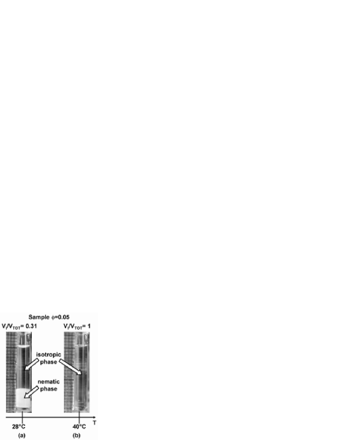
Figure 1: Pictures showing the phase separation of $5DH\mu em$. At low temperature (a) the system consists of a nematic phase filling 31 % of the total volume, coexisting with a lighter isotropic phase. At higher temperature (b) the system appears as a single isotropic phase.

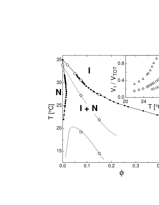
Figure 2: Experimental phase diagram featuring isotropic (I), nematic (N, grey shadowing) and phase coexistence (I+N). Full dots: phase boundaries obtained from the volumetric measurements shown in the inset. Open dots: $T_{DM}$ of the four samples used for volumetric measurements. Open diamond: extrapolated divergence temperature $T^{*}(\phi)$ of paranematic fluctuations. Open squares: extrapolated divergence temperature $T_{S}(\phi)$ for micellar density fluctuations. Inset: volume fraction of the isotropic phase in the two phase coexistence region for: $\phi=0.02$ (squares), $\phi=0.05$ (circles), $\phi=0.075$ (diamonds) and $\phi=0.15$ (triangles).

For temperature larger than the bulk $T_{NI}$, all the produced $5DH\mu em$ samples are optically isotropic. As T is lowered, a demixing phase transition takes place at a $\phi$ dependent temperature $T_{DM}(\phi)$. At $T<T_{DM}(\phi)$ samples separate into an isotropic phase coexisting with a denser optically uniaxial (nematic) phase. By maintaining the samples at constant temperature and waiting several hours, the two coexisting phases macroscopically separate under the effect of gravity. The samples appear as shown in Fig. 1 (a), where the highly scattering bottom nematic phase appears white. The two phases are easily distinguishable and the relative volume can be measured by taking pictures and analyzing the digital images. In order to extract from volumetric measurements the phase boundary of the coexistence region, we prepared - by successive dilution - four different samples: $s_{1}$ $(\phi=0.02)$, $s_{2}$ $(\phi=0.05)$, $s_{3}$ $(\phi=0.075)$, $s_{4}$ ($\phi=0.15$). These samples were kept into a thermostatic chamber with a stability of $\pm 5\cdot 10^{-3}K$ and observed by a digital camera at various temperatures. In the inset of Fig. 2 we show the T dependence of the ratio, $V_{I}/V_{TOT}$, between the volume of the isotropic phase and the total volume of the sample. Sample concentrations were chosen so that, in a wide temperature interval, at least two samples simultaneously have separated phases large enough to be easily measured (typically larger than $10\%$ of the total volume). At each temperature we have extracted the micellar weight ratios $\phi^{I}(T)$ and $\phi^{N}(T)$, enclosing the coexistence region of the $5DH\mu em$, shown as dots in Fig. 2.

In this analysis we have assumed that the behavior of $5DH\mu em$ can be understood as a pseudo-single component system, i.e. that micellar aggregates don’t change their structure as the phase transition takes place, but simply redistribute between the two phases. This assumption is confirmed by light scattering measurements in the isotropic phase, as discussed in the next Sections. Accordingly, from the standpoint of micelles, the phase transition is a simple demixing in which they preferentially accumulate in the isotropic phase. Since micelles are less dense than 5CB, their presence increases the density difference between isotropic and nematic phase.

II.3 Electric Birefringence Spectroscopy

Measurement of the Kerr coefficient have been performed by applying pulses of ac voltage. The pulse duration ($0.1-10ms$) was abundantly enough for the system to reach the steady state. The frequency $\nu$ of the applied field ranges from 1 kHz to 300 MHz, the upper limit being set by inductive loops introducing distortions in the detection of the field applied to the cell electrodes. For this reason the wiring has been designed to keep wire loops to a minimum. The field induced birefringence is, at steady state, composed by a dc component and by an ac component of frequency $2\nu$. While the former is related solely to the amplitude of the local dielectric anisotropy characterizing the nematic fluctuations in the isotropic phase, the latter is instead strongly dominated by the dynamics of the paranematic fluctuations. The set up used for these measurements is not equipped with a fast enough detection optics and transient digitizer to reliably measure the amplitude of the ac component. It is instead very accurate in the measurement of the dc component: the use of a quarter-wave plate in between cell and analyzer, the automated set-up enabling measurements at various angular positions of the analyzer and various field amplitudes, as well as the accumulation of a large number of pulse response at each studied frequency, allows extracting the field induced non oscillatory component of the birefringence $\Delta n_{dc}=n_{\parallel}-n_{\perp}$ with an error of few percent. The measured $\Delta n_{dc}$, has been found, as expected, to be proportional to the square of the electric field amplitude E, hence enabling a meaningful extraction of the Kerr constant $B(\nu)$ defined as:

$$B(\nu)=\frac{\Delta n_{dc}}{\lambda\langle E^{2}\rangle}$$ (1)

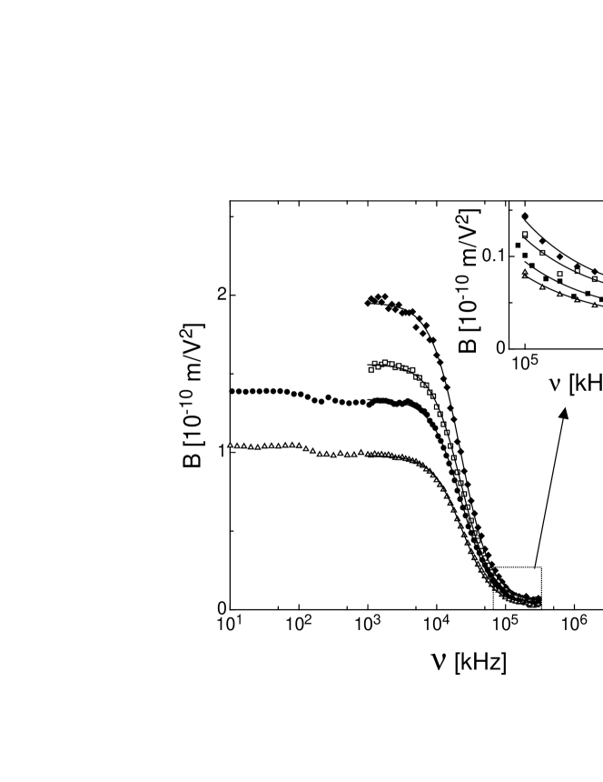
Figure 3: Electric birefringence spectra measured on a sample of bulk 5CB at various temperatures: $T=35.93^{\circ}C$ (triangles), $T=35.53^{\circ}C$ (dots), $T=35.28^{\circ}C$ (squares), $T=35.11^{\circ}C$ (diamonds). Lines: fittings with the Debye Eq. 4. Inset: enlargement of the high frequency data and fits.

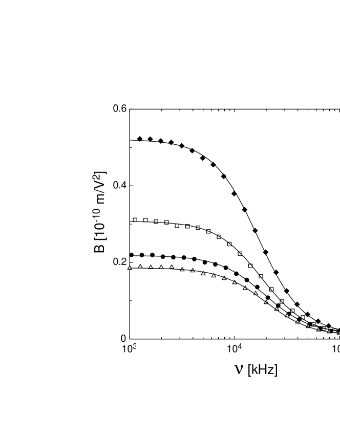
Figure 4: Electric birefringence spectra measured on a sample of $5DH\mu em$ with $\phi=0.15$ at various temperatures: $T=33.66^{\circ}C$ (triangles), $T=32.86^{\circ}C$ (dots), $T=31.85^{\circ}C$ (squares), $T=30.80^{\circ}C$ (diamonds). Lines: fittings with the Debye Eq. 4.

where $\lambda=633nm$ is the optical wavelength used in the experiment. In Figs. 3 and 4 we show $B(\nu)$ spectra measured in bulk 5CB and in a $5DH\mu em$ sample. As clearly visible, our experimental frequency range includes the main features of the spectra.

II.4 Static and Dynamic Light Scattering

Light scattering measurements have been performed by a highly automated experimental set up, featuring a He-Ne laser source, a temperature control with a $5\cdot 10^{-3}K$ stability and collection optics coupling scattered light into optical fibers. We used multimode fibers to measure the intensity of both polarized and depolarized scattered light ($I_{VV}$ and $I_{VH}$ respectively). Single mode fibers were instead used to measure intensity autocorrelation functions of the polarized and depolarized scattered light ($G_{2,VV}$ and $G_{2,VH}$, respectively). Use of fiber beam-splitter and cross correlation has enabled to reliably extract correlation functions down to a retardation time of 25 ns, a limit set by the electronics of the BI9000 correlator board used in the experiment. All static and dynamic measurements were performed at fixed angle $\theta=90^{\circ}$.

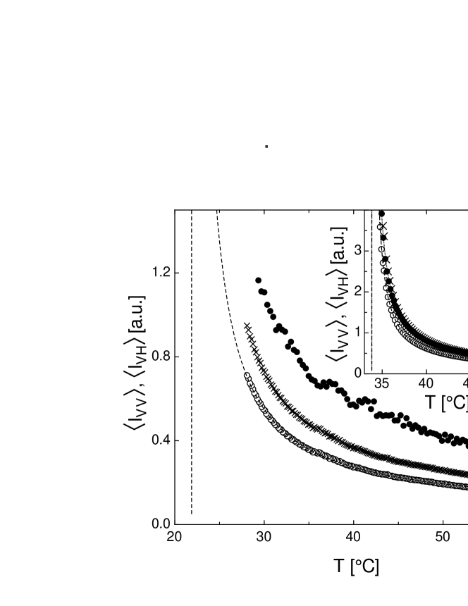
Figure 5: Scattered intensity in in a $5DH\mu em$ sample with $\phi=0.15$ (main figure) and in bulk 5CB (inset) as a function of temperature. Empty dots: depolarized scattered intensity $\langle I_{VH}\rangle$. Full dots: polarized scattered intensity $\langle I_{VV}\rangle$. Crosses: depolarized scattered intensity scaled by a $4/3$ factor (see Eq. 8). Lines: fittings with $(T-T^{*})^{-1}$. Main figure: $T^{*}=21.9^{\circ}C$, indicated by the vertical line. Inset: $T^{*}=33.8^{\circ}C$, for both the polarized and depolarized components.

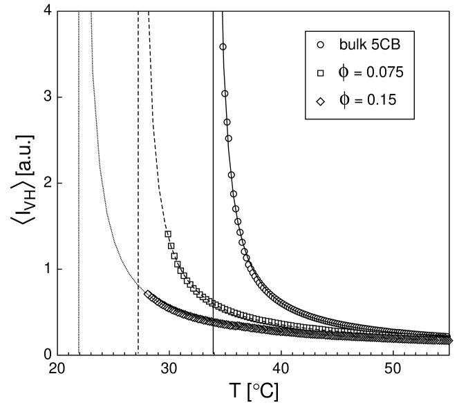
Figure 6: Comparison of the depolarized intensity scattered by bulk 5CB (circles) and $5DH\mu em$ with $\phi=0.075$ (squares) and $\phi=0.15$ (diamonds) as a function of temperature. Lines: fittings with $(T-T^{*})^{-1}$ yielding $T^{*}(bulk)=33.8^{\circ}C$ (solid vertical line), $T^{*}(\phi=0.075)=27.2^{\circ}C$ (dashed vertical line) and $T^{*}(\phi=0.15)=21.9^{\circ}C$ (dotted vertical line).

In Figs. 5,6 we show the polarized and depolarized scattered intensity for bulk 5CB and $5DH\mu em$ samples. While $I_{VV}$ and $I_{VH}$ measured in each sample at various T are on the same intensity scale, comparison between intensities scattered by different samples should be considered only as semi-quantitative since cell replacement required realignment of the collection optics.

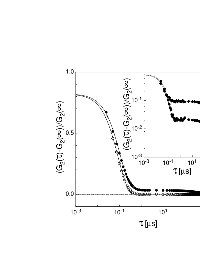
Figure 7: Normalized autocorrelation functions of the polarized (VV, full dots) and depolarized (VH, open dots) scattered intensities for the $\phi=0.075$ $5DH\mu em$ sample at $T=31^{\circ}C$. Inset: comparison of normalized autocorrelation functions of the polarized scattered intensity for the $\phi=0.075$ (full dots) and $\phi=0.15$ (diamonds) $5DH\mu em$ samples at $T=31^{\circ}C$. Lines: fit with double exponential decay (VV) and single exponential decay (VH)

Fig. 7 shows typical $G_{2,VV}$ and $G_{2,VH}$ measured by studying bulk $5DH\mu em$ samples. The inset of Fig. 7 instead compares $G_{2,VV}$ as measured in $\phi=0.075$ and in $\phi=0.15$ $5DH\mu em$.

III Description and analysis of the results

III.1 The phase diagram

The most relevant features of the phase diagram in Fig. 2 are the coexistence of a micelle poor nematic and a micelle rich isotropic over an extended temperature range and the presence of a re-entrant nematic phase.

It is known that inclusion of molecular dopants in a nematogenic compound results in extending the isotropic-nematic phase coexistence - confined to $T=T_{NI}$ in bulk LC - to a wide T interval. This phenomenon has been experimentally studied in detail for low contaminant dilution of aliphatic molecules having various shape pre8 . The authors also present a thermodynamic analysis of the $T_{NI}(\phi)$ slopes of the isotropic and nematic phase boundaries (approximated by straight lines converging to $T_{NI}$). In particular they showed that nematic-isotropic thermodynamic equilibrium implies that

$$\frac{1}{\beta_{N}}-\frac{1}{\beta_{I}}=\frac{\Delta S_{NI}}{R}$$ (2)

where $\beta_{N,I}=\frac{dT^{R}_{N,I}}{dx}$ are the are the slopes of the (respectively nematic and isotropic) phase boundaries enclosing the coexistence region, $T^{R}=\frac{T}{T_{NI}}$, $x$ is the contaminant concentration expressed in mole fraction, R is the gas constant and $\Delta S_{NI}$ is the N-I transition entropy for bulk 5CB that can be extracted from calorimetric measurements, namely $\Delta S_{NI}/R\sim 0.25$ pre8 .

According to Eq. 2, the quantity ($\beta_{N}^{-1}-\beta_{I}^{-1}$) is independent from the nature of the contaminant. Ref. pre8 reports that, for molecules of elongated shape, $\beta_{N}\sim-0.58$ and $\beta_{I}\sim-0.51$, thus approximately confirming the predicted behavior. A successive study of the effect on the I-N transition of 5CB doped by surfactant molecules of the polyoxethylene family reports $\beta_{N}\sim-1.35$ and $\beta_{I}\sim-0.95$ pre9 , also is agreement with Eq. 2.

The extrapolated initial slopes of the phase diagram in Fig. 2 are: $dT^{R}_{N}/d\phi\sim-1.23$ and $dT^{R}_{I}/d\phi\sim-0.20$. By assuming that all contaminants have the molecular weight of DDAB (i.e. disregarding the presence of water), we obtain $\beta_{N}\sim-2.6$ and $\beta_{I}\sim-0.35$, while, if we calculate exactly the total molar fraction of contaminants (water included) we obtain $\beta_{N}\sim-0.75$ and $\beta_{I}\sim-0.10$. In both cases the prediction of Eq. 2 is not confirmed since ($\beta_{N}^{-1}-\beta_{I}^{-1}$) is 10 to 30 times larger than predicted. Indeed, the $5DH\mu em$ phase diagram is evidently characterized by a separation between the isotropic and the nematic phase boundaries much larger than those found in refs pre8 and pre9 . This analysis suggests that, in calculating $\beta$, we are overestimating the molar concentration of dopants. Indeed, completely different estimates are obtained if one considers, as contaminants, not the single monomeric dispersed surfactant molecules, but the micellar aggregates, as discussed in section V after micellar sizes and interactions are introduced.

Although predicted by many previous theoretical analysis, the presence of a re-entrant nematic phase has been experimentally observed only quite recently pre10 by studying mixtures of the liquid crystal E7 and silicone oil. The nematic phase has been found to extend to a maximum contaminant concentration of 3 % vol. at about $10^{\circ}C$ below $T_{NI}$, i.e. similar but slightly larger than the one in Fig. 2. The physical origin of reentrant nematic phase can be sought in the combination of the positive T vs. $\phi$ nematic phase boundary expected at the lowest temperatures with the negative T vs. $\phi$ phase boundary resulting predicted for temperatures close to the NI transition. While at the limit of low temperature the nematic crystal expels all impurities, as T is increased the entropic gain for impurity solubilization determines an increment of the maximum micellar concentration in the N phase. Upon increasing further the temperature, the free energy difference between the bulk N and I phase is reduced, vanishing at $T_{NI}$. Therefore for each density of impurities solubilized in the nematic at low T, a maximum T is found where the free energy of the nematic with impurities equals the energy of the isotropic phase. At this temperature it pays for the system to phase separate into two phases as described by equation 2. The cross-over between the entropically driven impurity solubilization at low T and the impurity driven phase instability at high T leads to the observed reentrant behavior.

Phase diagrams similar to those in Fig. 2 have also been found in a somewhat different research contexts. The contaminant induced I-N phase separation is exploited to produce Polymer Dispersed Liquid Crystal materials. An isotropic mixture of isotropic LC and polymers is destabilized by a T quench. The isotropic phase hosting nematic nuclei is subsequently hardened by photo or chemically induced cross polymer linking. Such a phase separation has therefore received particular attention. Its experimental characterization, performed by studying a mixture of E7 and polybenzylmethacrylate pre11 , is qualitatively similar to the isotropic phase boundary in Fig. 2 although few experimental points may suggest the presence of an additional isotropic-isotropic phase separation.

III.2 Electric birefringence results

The onset of local nematic structuring, as the one predicted by Yamamoto and Tanaka’s ”transparent nematic”, would quite likely result in an electro-optic susceptibility larger than the conventional isotropic phase, as also suggested by the reported shear birefringence of such a phase. This is why measurements of electro-optic response by EBS appear particularly appropriate to study the $5DW\mu em$.

III.2.1 Bulk 5CB

According to the mean field description, the Kerr coefficient for bulk LC is given by pre12 :

$$B(\nu)=\frac{\epsilon_{0}\Delta\epsilon_{r}^{X}(\nu)\Delta n}{3\lambda a(T-T^{*})}$$ (3)

where $a$, $\Delta\epsilon_{r}^{X}$ and $\Delta n$ are, respectively, the first coefficient in the Landau-DeGennes expansion and the dielectric anisotropy and birefringence of a completely ordered nematic. $\Delta\epsilon_{r}^{X}=\epsilon_{\parallel}^{X}-\epsilon_{\perp}^{X}$, the parallel and perpendicular component of the dielectric coefficient of a perfectly ordered nematic (the superscript $X$ refer to nematic crystal), gauges the amplitude of the coupling of E with the induced nematic order, and is the only term in Eq. 3 depending on the frequency of the applied electric field. However, the contribution of $\epsilon^{X}_{\perp}$ to the frequency dependence of B is negligible: the permanent dipole of 5CB is aligned with the molecule and thus only electronic polarization contributes to $\epsilon^{X}_{\perp}$, which is therefore not expected to have observable frequency dependence in our experimental EBS spectra. The dominant contribution of $\epsilon_{\parallel}^{X}$ arises from molecular reorientation, its characteristic frequency deriving from the kinetics of molecular reorientation around the short axis. We thus expect EBS spectra for isotropic bulk 5CB to be close to its dielectric spectra.

In short, Eq. 3 indicates that EBS spectra enable accessing two independent quantities: the dynamics of the individual molecules from the frequency dependence of $B(\nu)$, and the degree of local paranematic ordering from the low frequency value of B. It is worth noticing that this last quantity cannot be detected by ordinary dielectric spectroscopy.

With respect to the more conventional pulsed electric birefringence, EBS better enables a distinction between the various processes taking place in the different frequency ranges. This is useful when low frequency artifacts, such as electrode polarization and space charge accumulations, typically frequency dependent, are present. In practice, our data, shown in Fig. 3, show little frequency dependence in the kHz regime. We have fitted, for $\nu>1$MHz the measured $B(\nu)$ with the sum of a frequency independent value, $B_{e}$, expressing the Kerr coefficient due to the anisotropy in the electronic polarization of 5CB molecules, and of a Debye type relaxation describing the frequency dependence of the polarization due to the reorientation of permanent dipoles:

$$B(\nu)=B_{e}+\frac{B_{d}}{1+(2\pi\frac{\nu}{\nu_{c}})^{2}}$$ (4)

In the fitting procedure, $B_{e}$, $B_{d}$ and $\nu_{c}$ are used as fitting parameters. The good quality of the fits indicates that a single relaxation frequency is enough to describe the whole polarization process. This may appear surprising since previous investigations by high frequency and time-domain dielectric spectroscopy on cianobiphenyls in the isotropic phase showed evident deviations from Debye behavior pre13 pre14 pre15 . In fact, Debye behavior is instead regularly observed when studying the $\epsilon_{\parallel}$ spectra in the nematic phase. We argue that, since $B(\nu)$ reflects the frequency dependence of $\epsilon_{\parallel}^{X}$, it is not actually unexpected that it behaves more similarly to the nematic $\epsilon_{\parallel}$ than to the isotropic $\epsilon$. This phenomenology together with more data on cianobiphenyls compounds, will be discussed in a forthcoming publication pre16 .

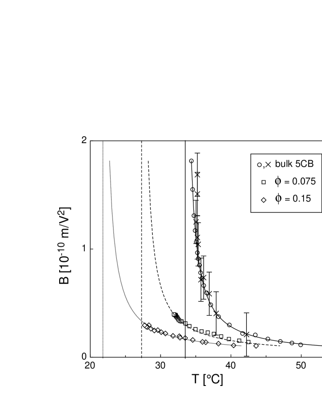
Figure 8: Low frequency Kerr constant $B$ of Bulk 5CB (circles) and $5DH\mu em$ with $\phi=0.075$ (squares) and $\phi=0.15$ (diamonds) as a function of temperature. Crosses: high frequency Kerr constant asymptote $B_{e}$ of bulk 5CB multiplied by a factor 15 to overlap $B_{d}$. Lines: fittings with $(T-T^{*})^{-1}$, as detailed in the text, yielding $T^{*}(bulk)=33.4^{\circ}C$ (solid vertical line), $T^{*}(\phi=0.075)=27.3^{\circ}C$ (dashed vertical line) and $T^{*}(\phi=0.15)=21.8^{\circ}C$ (dotted vertical line).

The three fitting parameters are found to depend on temperature. At all temperatures, we find that $B_{e}\sim B_{d}/30$. This ratio is in rough agreement with what expected by comparing dielectric $(\nu<\nu_{c})$ and optical $(\nu>\nu_{c})$ anisotropies: from literature values pre44 , in the nematic phase $(n_{\parallel}^{2}-n_{\perp}^{2})/(\epsilon_{\parallel}-\epsilon_{\perp})\sim 1/20$. The factor 1.5 in between estimate is probably due to the fact that our experiments are performed in the I phase, at values of field induce nematic order parameter much smaller than achievable in the N phase $(S(E=10V/mm)\sim 1\cdot 10^{-6})$ where the above ratio has instead been evaluated. The temperature dependence of $B_{e}$ and $B_{d}$ is shown in Fig. 8. As indicated, the uncertainty on $B_{e}$ is much larger than for $B_{d}$, and its T dependence has to be considered only qualitatively. In the same figure we have plotted the fit of $B_{d}(T)$ to $A_{5CB}(T-T^{*})^{-1}$, yielding $A_{5CB}=1.910^{-10}mV^{-2}$ and $T^{*}=33.4\pm 0.1^{\circ}C$. Both the quality of the fit and the value of $T^{*}$ in agreement to previous determinations, confirms that the amplitude of the Kerr effect is well described by a simple mean field theory.

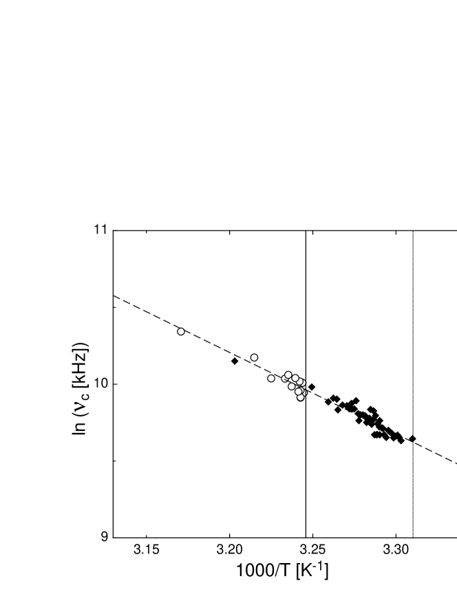
Figure 9: Arrhenius plot of $\nu_{c}$ vs. $1000/T$ for bulk 5CB (circles) and for $5DH\mu em$ sample with $\phi=0.15$ (diamonds). Dashed line: Arrhenius fit of all data. Vertical lines indicate $T_{NI}$ (solid line) and $T_{DM}(\phi=0.15)$ (dotted line).

In Fig. 9 we plot $\nu_{c}$ as a function of $1/T$. The Arrhenius-like behavior,

$$\nu_{c}\propto e^{(-\Delta H/RT)}$$ (5)

is evident, where $\Delta H$ is the activation energy. We find $\Delta H=41.0\quad kJ/mol$. This number should be compared with $\Delta H=33\quad kJ/mol$, obtained by fitting the Arrhenius dependence of the cut-off frequency of the 5CB dielectric spectra in the isotropic phase pre45 . According to mean-field expression, both EBS and dielectric characteristic frequencies should be proportional to the fluid viscosity pre55 . Such proportionality is partially confirmed when $\Delta H_{\epsilon}$ is compared with activation energy extracted from by the Arrhenius T dependence of 5CB viscosity: from literature we get: $\Delta H_{\eta}=29.0\quad kJ/mol$ pre19 , $\Delta H_{\eta}=44.9\quad kJ/mol$ pre20 , $\Delta H_{\eta}=28.3\quad kJ/mol$ pre21 . Despite the rather surprising numerical discrepancies, it is very clear from the data that EBS, in analogy to viscosity, probes the dynamical response of individual molecules, undergoing activated processes of angular reorientation. We will exploit the access to local molecular dynamics through EBS to evaluate how much the micellar inclusions affect the local viscosity, a notion necessary to interpret micellar diffusion.

III.2.2 $5DH\mu em$

As a simple inspection of the data in Fig. 8 immediately reveals, EBS results for the DDAB, water and 5CB mixtures are qualitatively similar to the bulk data although depressed in temperature and limited in amplitude. Although this is already enough to make clear that no extravagant molecular organization is present in the system, it is nevertheless interesting to analyze the results as it has been done for bulk 5CB.

All EBS spectra can be fitted with Debye dispersions (Eq. 4) as in the bulk. In Fig. 8 we show the low frequency Kerr coefficient $B_{d}$ as a function of temperature. The lowest value achieved for each given $\phi$ ($\phi=0.15$ and $\phi=0.075$) corresponds to the temperature at which demixing occurs, $T_{DM}(\phi=0.075)\sim 31^{\circ}C$ and $T_{DM}(\phi=0.15)\sim 27.5^{\circ}C$. In agreement with visual observations (section II.2), the isotropic phase of $5DH\mu em$ extends to temperatures lower than the bulk $T_{NI}$. By fitting $B_{d}$ to $A_{5CB}(1-\phi)/(T-T^{*})$, we obtain a value for $T^{*}$ depending on $\phi$, namely $T^{*}(\phi=0.075)=27.3^{\circ}C$ and $T^{*}(\phi=0.15)=21.8^{\circ}C$. As $\phi$ increases, the maximum value attained by the Kerr constant decreases, in agreement with the increased difference between $T_{DM}$ and $T^{*}$. These data, which will be discussed in Section III.3.2 together with the light scattering results, indicate that the electro-optic susceptibility of the mixture is dominated by the LC component and that its behavior is simply the one expected for an isotropic LC approaching the nematic transition with shifted $T^{*}$.

Since the individual molecular dynamics is typically unaffected by the onset of paranematic fluctuations pre22 , as also confirmed by our data for bulk 5CB, it is expected that the characteristic frequencies extracted from EBS $5DH\mu em$ would also not be influenced by pre-demixing phenomena. In Fig. 9 we plot $\nu_{c}$ vs. $1/T$ for the comparison with bulk results. Within the experimental uncertainty shown by the spread in the data point, the Arrhenius behavior of the $5DH\mu em$ $\nu_{c}$ data coincides with the bulk one, indicating that the activation energy for molecular reorientation is equal in the two systems. Thus the presence of the micelles doesn’t affect the molecular environment experienced by the LC molecules, which remains basically isotropic-like down to $T_{DM}$. Given the large fraction of 5CB molecules in contact with the DDAB molecules around the micelles (an estimate will be given in Section V), this result clearly indicates that no significant anchoring of LC molecules is induced at the micelle-LC interface.

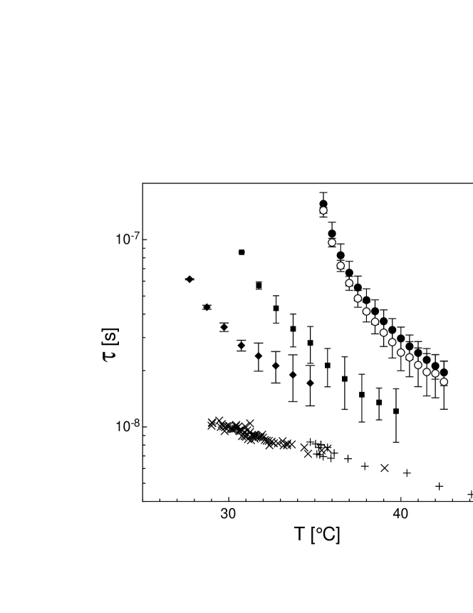
Figure 10: Comparison between characteristic times and inverse frequencies characterizing the dynamic light scattering and electric birefringence spectra. Full dots: $\tau_{PN,VV}$ for bulk 5CB. Empty dots: $\tau_{PN,VH}$ for bulk 5CB. Squares: $\tau_{PN,VH}$ for the $\phi=0.075$ $5DH\mu em$. Diamonds: $\tau_{PN,VH}$ for the $\phi=0.15$ $5DH\mu em$. Pluses: $1/(2\pi\nu_{c})$ for bulk 5CB. Crosses: $1/(2\pi\nu_{c})$ for the $\phi=0.15$ $5DH\mu em$

In Fig. 10 we show the characteristic time $\tau_{c}=(2\pi\nu_{c})^{-1}$ extracted from the data in Fig. 9, to be compared with the characteristic time for paranematic fluctuations, as discussed below.

III.3 Light Scattering Results: Extracting Paranematic and Micellar Contributions

III.3.1 Bulk 5CB

Light scattering provides valuable information on both the statics and dynamics of pretransitional paranematic fluctuations through, respectively, the intensity and the correlation function of the scattered light. Because of the first order nature of the I-N phase transition, light scattering results are usually accurately described by the mean field theories. Accordingly, the scattered intensity, as described by the Rayleigh ratio R, grows as pre22

$$R=\frac{k_{B}T}{a(T-T^{*})}$$ (6)

while the correlation time of the paranematic fluctuations is given by pre22

$$\tau_{PN}=\frac{k_{B}T\eta}{a(T-T^{*})}$$ (7)

where $\eta$ is the viscosity.

Our bulk data are in agreement with the mean field description and with previous investigations. Measured $I_{VV}$ and $I_{VH}$ intensities are well fit by Eq.6 with added a background constant, accounting for stray light. Fig. 6 shows such a fit for $I_{VH}$, yielding $T^{*}=33.8^{\circ}C$ (and thus $T_{NI}-T^{*}=0.9^{\circ}C$), in acceptable agreement with literature pre17 and EBS data analysis. Polarized and depolarized intensity are found to be proportional, as predicted pre22 :

$$\langle I_{VH}\rangle=\frac{3}{4}\langle I_{VV}\rangle$$ (8)

This is shown in Fig. 5 where cross symbols represent $\frac{4}{3}\cdot\langle I_{VH}\rangle$ and nicely overlay on $\langle I_{VV}\rangle$ data.

The correlation functions obtained in the bulk can be well fit with exponential decays. The analysis of the $VV$ correlation functions yields to values of $\tau_{PN}$ (see Fig. 10, full dots) about 15 % larger than those obtained from VH scattering. This observation is in line with prediction in the frame of mean field analysis as a consequence of coupling between shear viscosity and density fluctuations, which bears detectable effects in the VH Rayleigh spectra pre22 . On the basis of equation (23) of Ref. pre22 and by using values obtained from experiments on MBBA, we would predict $\tau_{PN,VV}/\tau_{PN,VH}\sim 1.3$, about double of what observed in 5CB.

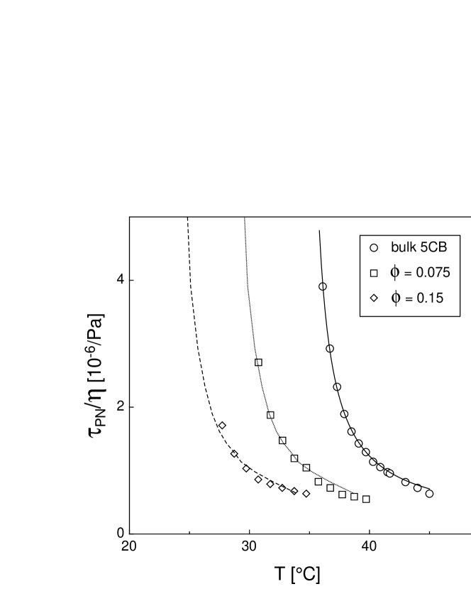
Figure 11: Paranematic correlation time $\tau_{PN}$ divided by the shear viscosity $\eta$ for bulk 5CB (circles) and $5DH\mu em$ with $\phi=0.075$ (squares) and $\phi=0.15$ (diamonds) as a function of temperature.

$\tau_{PN}/\eta$ can be well approximated by $(T-T^{*})^{-1}$, as predicted by Eq. 7 and shown in Fig. 11. The extracted divergence paranematic temperature is $T^{*}=34.4^{\circ}C$ is too high with respect to the one obtained from $I_{PN}$ in the same light scattering experiment. The origin of this difference appears to be seeded in the behavior of $\eta$ pre16 .

III.3.2 $5DH\mu em$

Microemulsion data require some additional analysis. The measured correlation functions (Fig.7) very clearly demonstrate the presence of two distinct processes: a fast one, appearing in both VV and VH correlations, clearly due to paranematic fluctuations, and a slower one, appearing only in the VV correlations, detectable only in the microemulsions. This last component, indicating the presence of aggregates within the 5CB matrix, is easily interpreted as intensity scattered by the inverted micelles. Thus the total scattered intensity $I_{TOT}=I_{PN}+I_{M}$ is the incoherent sum of intensity scattered by LC orientational fluctuation ($I_{PN}$) and by micelles ($I_{M}$). Specifically

$$I_{VV}\equiv I_{TOT,VV}=I_{PN,VV}+I_{M}$$ (9)

while

$$I_{VH}\equiv I_{TOT,VH}=I_{PN,VH}$$ (10)

The large difference between the correlation times of the two components makes it possible to identify them. Let’s indicate with $\tau_{mid}\sim 1-10\mu s$ a correlation time long with respect to paranematic fluctuation time and short with respect to micellar diffusional times. Because of the statistical independence of the two terms we have

$$\begin{array}[]{ll}G_{2,VV}(0)-G_{2,VV}(\tau_{mid})&=c(\langle I_{PN,VV}^{2}\rangle+2\langle I_{PN,VV}\rangle\langle I_{M}\rangle)\\ G_{2,VV}(\tau_{mid})-G_{2,VV}(\infty)&=c\langle I_{M}^{2}\rangle\end{array}$$ (11)

where $c$ is a factor related to the collection optics. Combining the two equations, $\langle I_{M}\rangle$ can be derived from the total polarized scattered intensity and from the decay of the correlation functions. Alternatively, $\langle I_{M}\rangle$ can be extracted from the polarized scattered intensity $\langle I_{VV}\rangle$ as

$$\langle I_{M}\rangle=\langle I_{VV}\rangle-\frac{4}{3}\langle I_{VH}\rangle$$ (12)

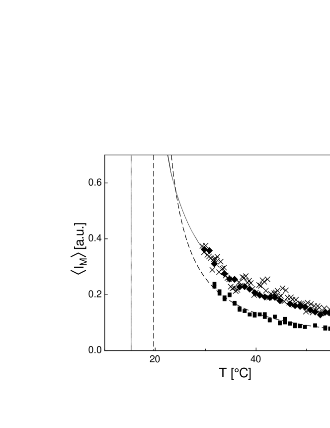
Figure 12: Intensity scattered by microemulsion droplets $\langle I_{M}\rangle$ extracted from dynamic light scattering data as a function of temperature. Squares: $\phi=0.075$. Diamonds: $\phi=0.15$. Crosses: $\langle I_{M}\rangle$ obtained from the difference between $I_{VV}(\phi=0.15)$ and $4/3\cdot I_{VH}(\phi=0.15)$ and normalized to match diamonds at $T=60^{\circ}C$. Lines: fittings with $(T-T_{S})^{-1}$ yielding $T_{S}(\phi=0.075)=19.4^{\circ}C$ (dashed vertical line), $T_{S}(\phi=0.15)=14.6^{\circ}C$ (dotted vertical line)

where we have used the notion that $\langle I_{PN,VV}\rangle=4/3\langle I_{VH}\rangle$ as observed for paranematic scattering in bulk 5CB (eq. 8). Fig. 12 compares the values of $\langle I_{M}\rangle$ vs. T obtained from the two procedures. The comparison clearly confirms that the T dependence of $\langle I_{M}\rangle$ is indeed reliably extracted. The determination of $\langle I_{M}\rangle$ from DLS data, however, requires extracting $G_{2,VV}(0)$ from the correlation functions. This has been done by fitting $G_{2,VV}(\tau)$ by a sum of two exponentials (see Fig. 7) enabling determining $G_{2,VV}(0)$, as well as $\tau_{PN}$ and the micellar correlation time $\tau_{M}$. $\tau_{PN}$ obtained from $G_{2,VH}(\tau)$ are more reliable than those obtained from $G_{2,VV}(\tau)$ since in this last case the intensity scattered by the micelles, basically constant on the times scale of paranematic fluctuations, beats with the light diffused by orientational fluctuations thus introducing an heterodyne contribution to the correlation function. Therefore, $\tau_{PN}$ extracted from $G_{2,VV}(\tau)$ would, in principle, require a compensating correction, unnecessary in the VH scattering. Although in practice such a correction is small since $I_{M}/I_{LC}<15\%$ always, we will in the following refer to $\tau_{PN}$ obtained from $G_{2,VH}(\tau)$.

In summary, light scattering measurements enable extracting $\langle I_{PN}\rangle$ , $\langle I_{M}\rangle$ , $\tau_{PN}$, $\tau_{M}$ as a function of T and for the different samples. In what follows we will separately discuss results pertaining the two sides of the $5DH\mu em$ behavior: LC in the presence of nanoinclusions and micelles within a solvent with ordering fluctuations.

Inspection of $\langle I_{PN}\rangle$ vs. T measured in the $5DH\mu em$ shown in Fig. 6 reveals that: (i) at any given T, paranematic fluctuations are depressed by the presence of the micelles; (ii) an isotropic phase like behavior extends down to $T_{DM}$, i.e. even at T lower than the bulk $T_{NI}$; (iii) the maximum value of $\langle I_{PN}\rangle$ for each given preparation, obtained for $T=T_{DM}$, is a decreasing function of $\phi$.

By fitting $I_{PN}(T)$ as for the bulk data we obtain $T^{*}(\phi=0.075)=27.2^{\circ}C$ and $T^{*}(\phi=0.15)=21.9^{\circ}C$, closely matching the results obtained from EBS. These results are reported in the phase diagram in Fig. 2, where the dotted line interpolating the data guesses the behavior of $T^{*}(\phi)$.

$\tau_{PN}/\eta$ data vs. T are shown in Fig. 11. Given the uncertainty on the T dependence of the viscosity, as discussed above, we prefer not to fit the data, but to evaluate the magnitude of the temperature shift induced by the presence of the micelles by finding the best overlap between the $5DH\mu em$ data and the bulk 5CB data shifted down in temperature of $\delta T$ as shown in Fig. 11. Best overlaps have been obtained with $\delta T=6.25^{\circ}C(\phi=0.075)$ and $\delta T=11.0^{\circ}C(\phi=0.15)$, to be compared, respectively, with $T^{*}(bulk)-T^{*}(\phi=0.075)=6.6^{\circ}C$ and with $T^{*}(bulk)-T^{*}(\phi=0.075)=11.9^{\circ}C$ as obtained in static LS.

The overall agreement between the $T^{*}$ from static and dynamic LS and from the low frequency Kerr measurements, supports the notion that the annealed disordering provided by the micelles is affecting the LC behavior simply by shifting it to lower temperatures and by increasingly precluding the development of paranematic fluctuations by the appearance of the demixing transition, i.e. $T_{DM}(\phi=0.15)-T^{*}(\phi=0.15)[\sim 10^{\circ}C]>T_{DM}(\phi=0.075)-T^{*}(\phi=0.075)[\sim 6^{\circ}C]>T_{NI}-T^{*}(bulk)[\sim 1^{\circ}C]$.

III.3.3 Micellar behavior

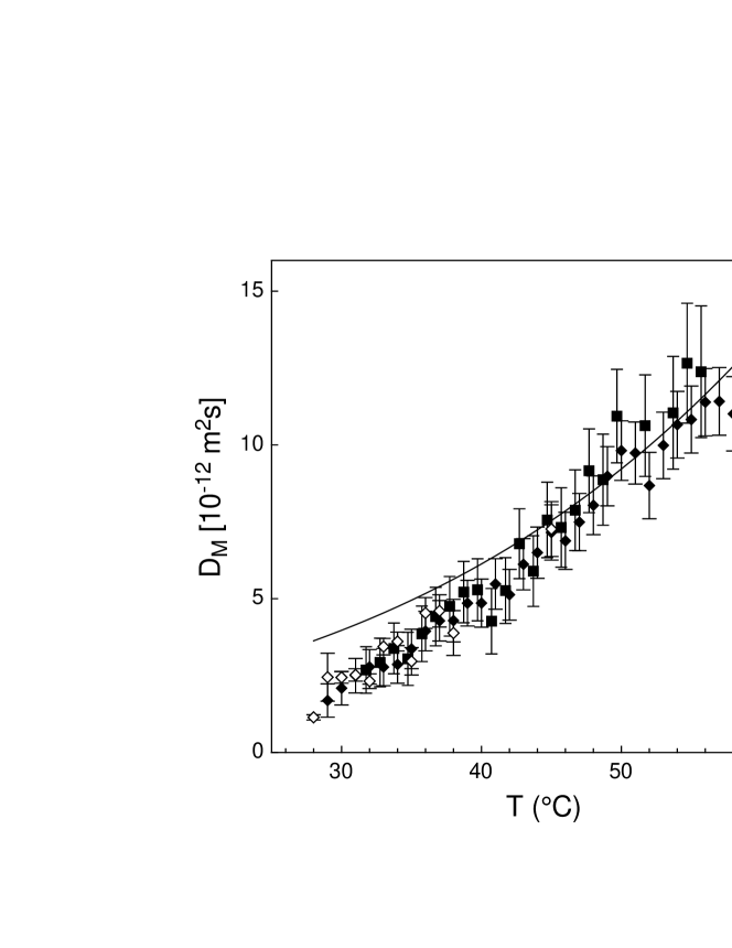
Figure 13: Micellar diffusion coefficients $D_{M}$ as a function of temperature for $5DH\mu em$ samples with $\phi=0.15$ (full diamond), $\phi=0.075$ (squares). Empty diamonds $D_{M}$ measured in the upper phase of a $\phi=0.075$ $5DH\mu em$ at $T=27^{\circ}C$ where independent estimates indicate a micellar concentration of $\phi=0.14$. Line: expected temperature dependence of $D_{M}$ for non interacting microemulsion droplets having radius $R=18\mbox{\AA}$ calculated on the bases of $\eta(T)$ from Ref. pre20 .

The temperature dependence of $\langle I_{M}\rangle$ for the two concentrations is shown in Fig. 12. The most interesting characteristic of these data is the growth of $\langle I_{M}\rangle$ as T decreases, which cannot be understood simply in terms of T dependence of refractive indices, which, in the T interval of Fig. 12, vary at most by 1 %. Analogous deviation from simple behavior is observed in the diffusion dynamics of the micelles. The micellar diffusion coefficient $D_{M}$ extracted from $\tau_{M}^{-1}=2D_{M}q^{2}$ (where $q$ is the scattering vector) is shown in Fig. 13 and compared with the $D_{M}$ which would be expected from the Einstein equation $D_{M}=(k_{B}T)/(6\pi\eta R)$ in the case of spheres of radius $R=18\mbox{\AA}$ diffusing in the isotropic phase, where the viscosity is taken from Ref. pre20 . The radius has been chosen so to approximate the observed $D_{M}$ at the highest measured temperatures. As evident from the comparison, in the proximity of the demixing transition, the measured dynamics is slower than the expected one by a factor of about 2 in both the $\phi=0.15$ and the $\phi=0.075$ samples.

The comparison between $D_{M}(T,\phi)$ and $(k_{B}T)/(6\pi R\eta(T))$ is based on the assumption that the local viscosity experienced by inverted micelles in the $5DH\mu em$ is unchanged with respect to bulk 5CB and that, for $T<T_{NI}$, where no bulk data for isotropic viscosity exists, $\eta(T)$ is given by the same Arrhenius dependence as in the bulk. This assumption is is based on our EBS results on the Kerr $\nu_{c}$, which proved that the local molecular environment in the isotropic phase of $5DH\mu em$ overlaps the low T extrapolation of the bulk Arrhenius. Given that viscosity and molecular diffusion share their basic physical origin pre23 , we conclude that similar T dependence is expected for $\eta(T)$. Use of another among the published 5CB viscosities would not change the comparison in Fig. 13. Namely, by using $\eta(T)$ as in Ref. pre19 we would obtain $R=21\mbox{\AA}$ and a maximum ratio between expected and measured D of about $2.1$, while by using $\eta(T)$ as in Ref. pre21 we would obtain $R=24\mbox{\AA}$ and a maximum ratio between expected and measured $D_{M}$ of about $1.8$. Given this dispersion of the R values, in the following discussion we will assume $R=20\pm 2\mbox{\AA}$.

According to our data, and within our experimental error, the diffusion coefficients measured for the two $5DH\mu em$ micellar concentrations vs. T are basically the same (see Fig. 13). Although this result may appear as a straightforward indication of having droplets of the same size in the two samples, some analysis is instead required. In fact, $\phi=0.15$ is a rather significant volume fraction, at which effect from interparticle interactions may be expected. When expressed through the virial expansion pre35 , the collective diffusion coefficient measured at a given particle concentration is

$$D_{M}=D_{M,0}(1+k_{D}\phi)$$ (13)

where $D_{M,0}$ is the diffusion coefficient at infinite dilution and $k_{D}$ is the virial coefficient expressing the correction to collective diffusion arising from interparticle interactions. According to the data here presented, the product $k_{D}\phi$ assumes the same value in the two different samples, thus indicating a $\phi$ independent D, and possibly $k_{D}=0$.

In order to check the robustness of this evidence and also to explore possible deviations from simple one-component Maxwell rule for the phase coexistence, we have studied the upper phase - denser in micelles - obtained by letting a $\phi=0.075$ sample separate at $T=27.5^{\circ}C$. The resulting micellar volume fraction, calculated from the volume ratio of the phases and assuming a 2 % micelles in the lower N phase (see Fig. 2) was $\phi=0.14$. Dynamic light scattering measurements on the upper isotropic phase are possible because the time for the two coexisting phases to remix is much larger than the time to perform the experiment. The micellar diffusion coefficient obtained in this way is compared in Fig 13 with the $D_{M}$ measured in sigle phase $5DH\mu em$. The overlap of the data confirms the absence of significant concentration dependence of $D_{M}$ at least within our experimental error. Moreover it supports the single component approximation, previously assumed in drawing the phase diagram (see Section II.2).

The deviation of $D_{M}(T)$ from $k_{B}T/\eta(T)$ indicates that the product $k_{D}\phi$ , constant for $T>40^{\circ}C$, grows appreciably as the system approaches the demixing transition. Altogether, the matching of $D_{M}(T)$ with $k_{B}T/\eta(T)$ at high T, and the independence of $k_{D}\phi$ on $\phi$ , strongly suggests that, at high enough temperature, $k_{D}\sim 0$. Vanishing virial coefficients are not at all a surprise for water in oil microemulsions. Systematic investigations in systems prepared with different choices of oil and surfactants have revealed that inverted micelles may interact with a wide range of variable strengths, ranging from negative - hard sphere like - to positive virial coefficient pre25 . This is reflected in other studies too. In one of them pre26 , it was found that a large body of data could be satisfactorily understood on the basis of hard sphere repulsion, with the hard sphere radius few Å smaller than the measured hydrodynamic radius. Other investigations pre27 ; pre28 concluded that contact attractive interactions had to be included to interpret the data. In another study pre29 it was actually found that collective diffusion was independent on droplet concentration, as in the $5DH\mu em$ case here. The existence of attractive interactions in inverted micelles is usually attributed to an entropic gain coming into play when the hydrophobic tail of the surfactants of two droplets overlap pre30 . Our data indicate that such a ”stickiness” interaction may be present in our system to compensate, as far as $k_{D}$ is concerned, for the hard sphere repulsion of the hydrophilic cores, certainly present. Thermal dependence of such interpenetration interaction also explains the inverted consolution curve (”lower” critical solution temperature) observed in the water-AOT-octane pre30 ; pre31 . We stress that such inverted demixing (induced upon increasing T) is the only gas-liquid like phase separation observed in water-in-oil microemulsions and that its reversed nature clearly demonstrates that the demixing observed in $5DH\mu em$ (induced upon lowering T) cannot be explained by the same attractive potential.

Previous works on DDAB pre32 , focused on w/o microemulsions prepared by using hydrocarbon oils and with a much higher water/DDAB concentration ratio, propose a calculation scheme for the micellar size which would yield, in our case $R\sim 15.5-19.5\mbox{\AA}$, depending on how extended the DDAB chains are. Care should be taken, though, since the radius may depend on the nature of the oil. By comparing phase diagrams obtained with different kind of oils, two interesting elements appear: (i) DDAB is insoluble in alkanes if no water is added, indicating the existence of a minimum curvature of the DDAB layer, which also appears to be dependent on the alkane chain length pre32 ; pre33 ; (ii) DDAB is soluble in toluene with no added water but it does not form micelles pre24 . DDAB is soluble in the isotropic phase of 5CB with no added water. However, DLS measurements have revealed that, at variance with the toluene system, DDAB in the isotropic phase of 5CB form micelles. Their radius, measured in a sample with 15 % DDAB in 5CB by a different DLS set-up equipped by a more powerful laser source, is $R\sim 18\mbox{\AA}$. This number should be considered as very approximate because no analysis has been done on possible intermicellar interactions. Overall, the solubility properties of DDAB in 5CB appears to be quite different from that in both alkanes and toluene.

A simple estimate of the $5DH\mu em$ inverted micellar structure is as follows. By assuming an intermediate (not fully extended) DDAB hydrocarbon chain length of $14\mbox{\AA}$ pre32 , it follows that the water core radius $R_{W}\sim 6\mbox{\AA}$. Since the DDAB/water volume ratio extends to the micellar structure, should the DDAB not compenetrate with 5CB molecules but rather form a compact spherical shell, we would have micelles of $13.5\mbox{\AA}$. This fact suggests a very strong interfingering of DDAB and 5CB molecules, in agreement with what implied by the solubility of DDAB in 5CB and by the large curvature of DDAB in 5CB. Overall, the DDAB volume in every droplet is small, and corresponds to about 13-14 DDAB molecules.

III.3.4 Micellar concentration fluctuations

The growth of $\langle I_{M}\rangle$ and of $D(T)\eta(T)/k_{B}T$ as $T_{DM}$ is approached could, in principle, be explained in a variety of manners. It could be due to the growth of a 5CB layer of radially anchored molecules on the micelles surface, thickening as a consequence of the increasing nematic correlation length. Alternatively, it could follow from restructuring of the spontaneously assembled water-DDAB droplets. Finally, it could reflect the onset of attractive intermicellar forces. We will argument in favor of this last explanation.

The development of a radial nematic layer around the micelles could certainly bring about a slowing down of their diffusion, but it certainly would not increase their scattering cross section for light. Indeed, given the size of the particles - well within the Rayleigh scattering regime pre34 , isotropically anchored molecules cannot be distinguished from a layer of isotropically distributed unanchored molecules.

Restructuring of the self-aggregated nanodroplet could take place but only allowing for non-spherical shapes, since the ratio [DDAB]/[water] has to be maintained in any aggregate. In order to account for a growth of about a factor 3 in the scattered intensity, aggregates should increment their volume of about 3 times. This would lead to the formation of rod-like micelles whose diffusion coefficient can be explicitly calculated and results to be at least 4 times larger than expected for spheres of constant radius. Since the observed slowing down is only of a factor 2, we don’t see room for pursuing this explanation.

Interparticle attraction, besides slowing down their diffusion, also give rise to concentration fluctuations, in turn enhancing the amount of scattered light. This effect is described by the second virial coefficient $k_{I}$ in the virial expansion

$$I_{M}=I_{M,0}(1+k_{I}\phi)^{-1}$$ (14)

where $I_{M,0}$ is the scattered intensity measured if interactions were not present. $k_{D}=k_{I}-k_{f}$, where both $k_{D}$ and $k_{f}$ are suitable integrals of the pair potential pre35 . While $k_{I}$ describes concentration fluctuations, $k_{f}$ takes into account hydrodynamic interactions. Attractive interactions correspond to negative coefficients. For short ranged potentials, $k_{f}$ has typically the same sign of $k_{I}$ but is smaller in amplitude (about half or less). $\langle I_{M}\rangle$ data in Fig. 12 are extracted from $\langle I_{VV}\rangle$ data on the basis of the ratio of slow and fast dynamics in the intensity correlation functions. Thus, as in the case of $I_{VV}$ , the values of $\langle I_{M}\rangle$ cannot be compared between different samples. However, the fact that $k_{D}\sim 0$ at high temperature, suggests that also $k_{I}$ is negligible in the same temperature range, as found in other systems having vanishing $k_{D}$ pre35 . The growth of $\langle I_{M}\rangle$ as T decreases indicates that $k_{I}$ is temperature dependent, ranging from its ”high T” value $k_{I}^{HT}=0$, to a value at the demixing temperature $k_{I}\sim-4.3$ in the case of $\phi=0.15$ and a value $k_{I}\sim-9.3$ in the case of $\phi=0.075$ (from the data in Fig. 12).

Since an increment in the attractive potential implies an increment in the negative value of both $k_{I}$ and $k_{f}$, with the second smaller in modulus than the first, we expect $k_{D}$ to be negative and $k_{D}>k_{I}$. This prediction is in agreement with the experimental result, in which the effects of interactions are more conspicuous in the scattered intensity than in the diffusion coefficient. Therefore, while neither the growth of a nematic layer around the droplets nor micellar restructuring results compatible with experimental results, the appearance of intermicellar attraction is capable to account for the data.

Although the specific nature of intermicellar interactions is not experimentally accessible, their occurrence in the proximity of the demixing transition, in a temperature interval in which orientational fluctuations also develop, suggests the existence of a connection between the two phenomena. It is exactly to explore such a connection that we have developed the model described in the following Section.

IV Theoretical model

The nematic phase can be modelled in a variety of ways, having various degrees of realism. Striking, for its simplicity and effectiveness in capturing the strength of the first order I-N phase transition, is the Lebwhol-Lasher (LL) model pre40 , a spin lattice model with the simplest orientational coupling compatible with the non-polar nematic symmetry. This model is also interesting because it enables studying the effects of quenched disorder once a random field is properly added pre47 ; pre48 . Hence, the LL model appears as an attractive starting base to investigate the effect of nanoimpurities. The LL model can also be reckoned as the lattice counterpart of the widely known Maier-Saupe model pre57 ; pre58 , which has been repeately studied ever since pre59 .

The analysis of the pretransitional behavior of the pure LL indicates that, if a mapping is attempted between spins and molecules, a single spin represents not a single molecule but rather a cluster of about 50 molecules pre49 . In the case of $5DH\mu em$, the droplets in the solution are comparable in sizes with the length of the LC molecules, while filling the volume of 20-40 5CB molecules. Hence, one is then led to suspect that a lattice model containing a mixture of LC and micelles, taken to be of the same size, might be sufficient to capture the main qualitative features of the experiments presented so far. We now show that this is indeed the case. In our model, LC are represented by pointless unit vectors $\hat{s}$ which are free to rotate in three dimensional space, but are fixed in position to a lattice of spacing $a$:

$$\hat{s}=(s^{1},s^{2},s^{3})=(\sin{\theta}\cos{\phi},\sin{\theta}\sin{\phi},\cos{\theta})$$ (15)

Micelles, on the other hand, are simply mimicked by vacancies, and are then represented - in the spirit of a lattice gas model - by a lattice variable $\sigma=0(,1)$ when the lattice site is vacant (occupied by LC).

As usual, it proves convenient to introduce the traceless quadrupole tensor

$$Q^{\alpha\beta}(\hat{s})=\frac{1}{2}(3s^{\alpha}s^{\beta}-\delta^{\alpha\beta})\qquad\qquad\alpha,\beta=1,2,3$$ (16)

The final Hamiltonian then reads:

$$-\beta H=K_{qq}\sum_{\alpha\beta}\sum_{\langle xy\rangle}Q_{x}^{\alpha\beta}Q_{y}^{\beta\alpha}\sigma_{x}\sigma_{y}+K_{\sigma\sigma}\sum_{\alpha\beta}\sum_{\langle xy\rangle}\sigma_{x}\sigma_{y}\\ +\sum_{\alpha\beta}\sum_{x}h_{x}^{\alpha\beta}Q_{x}^{\alpha\beta}\sigma_{x}-\sum_{x}\beta\mu\sigma_{x}$$ (17)

Here the first term reflects the fact that two LC have the general tendency to align along a common direction with coupling $K_{qq}=\beta J_{qq}$, $(\beta=1/k_{B}T)$, the second term is a standard lattice gas Ising-like interaction with coupling $K_{\sigma\sigma}=\beta J_{\sigma\sigma}$, and the next two terms correspond to the external fields ($h^{\alpha\beta}$ for the LC and $\mu$ for the micelles) controlling the LC orientation and micelle concentrations respectively.

In the following the average fraction of micelles will be denoted as $\phi$. It is worthwhile noticing that in Eq (17) the micelles interact both directly (through a $K_{\sigma\sigma}$ coupling) and indirectly, because of the presence of the LC. As we shall show, the latter are responsible for the most interesting features of the mixture, and are present even in the absence of the former.

IV.1 Mean Field Analysis

The diluted LL model has been studied using Monte Carlo simulations pre60 ; pre61 In the following we shall study it within a mean field approximation akin that of its continuum counterpart pre59 .

To this aim we define a trial Hamiltonian

$$-\beta H_{0}=\sum_{\alpha\beta}\sum_{x}b_{x}^{\alpha\beta}Q_{x}^{\alpha\beta}\sigma_{x}+\sum_{x}\lambda_{x}\sigma_{x}$$ (18)

where $b^{\alpha\beta}$ and $\lambda$ are variational parameters for the LC and micelles respectively. As remarked, at variance of Ref. pre7 , we shall exploit an Hamiltonian which is not simply factorized in two terms which depend on one variable only. Clearly a more general choice

$$\tilde{H}_{0}=\sum_{x}h\left(\{Q\sigma_{x}\}\right)$$ (19)

($h\left(\{Q\sigma_{x}\}\right)$ being a single site hamiltonian) could be exploited, but the calculations quickly become analytically unmanageable.

Accordingly we shall use the following order parameters

$$q_{x}^{\alpha\beta} = \left\langle Q_{x}^{\alpha\beta}\sigma_{x}\right\rangle$$ (20)

$$n_{x} = \left\langle\sigma_{x}\right\rangle$$

where averages are over the trial Hamiltonian. Note that $\phi=1-n$.

The calculation now follows standard procedures. Once the mean field free energy $\beta F_{MF}$ has been obtained, it proves convenient to Legendre transform to a mixed function

$$\beta\Gamma_{MF}=\beta F_{MF}+\sum_{x}h_{x}^{\alpha\beta}q_{x}^{\alpha\beta}+\sum_{x}\mu^{*}_{x}n_{x}$$ (21)

where $\mu^{*}=\beta\mu$. This function clearly depends upon the variational parameters $b^{\alpha\beta}$ and $\lambda$, whose explicit values are obtained by the requirement that the free energy is stationary at those values. The final results for this mixed free energy in terms of the homogeneous value of the micelles order parameter $n$ and of the LC order parameter $q$ as identified by the diagonal matrix

$$q^{\alpha\beta}=\begin{vmatrix}-\frac{q}{2}&0&0\\ 0&-\frac{q}{2}&0\\ 0&0&q\end{vmatrix}$$ (22)

is

$$\frac{\beta\hat{\Gamma}_{MF}(q,n)}{N} = \frac{9}{2}K_{qq}q^{2}-3K_{\sigma\sigma}n^{2}+\frac{9}{2}K_{qq}qn+$$

$$+n\log{n}+(1-n)\log{(1-n)}-\log{4\pi}-n\log{\left[I_{0}\left(\frac{27}{2}K_{qq}q\right)\right]}$$

where we have defined the integrals

$$I_{n}(\lambda)=\int_{0}^{1}dx~{}x^{n}e^{\lambda x^{2}}$$ (24)

IV.1.1 The phase diagram

The isotropic-nematic transition is obtained by the conditions (when $h^{\alpha\beta}=0$)

$$\frac{\partial}{\partial q}\left[\frac{\beta\hat{\Gamma}_{MF}}{N}\right] =0$$ (25)

$$\frac{\partial}{\partial n}\left[\frac{\beta\hat{\Gamma}_{MF}}{N}\right] =-\mu^{*}$$

that is:

$$q = n\Phi\left(\frac{27}{2}K_{qq}q\right)$$ (26)

$$\mu^{*} = 6K_{\sigma\sigma}n-\frac{9}{2}K_{qq}q-\log\left(\frac{n}{1-n}\right)+\log{\left[I_{0}\left(\frac{27}{2}K_{qq}q\right)\right]}$$ (27)

where

$$\Phi(\lambda)=-\frac{1}{2}+\frac{3}{2}\frac{I_{2}(\lambda)}{I_{0}(\lambda)}$$ (28)

Note that the Eq.(27) is a self-consistency equation for the nematic order parameter $q$.

It is instructive to compare the above results with the corresponding one obtained in the absence of micelles, i.e. the fully occupied Lebwohl-Lasher model (FLL), and with the simple lattice gas case. The free energy for the former reads

$$\left[\frac{\beta\hat{\Gamma}_{MF}(q)}{N}\right]_{FLL} = \frac{9}{2}K_{qq}q^{2}+\frac{9}{2}K_{qq}q-\log(4\pi)-\log\left[I_{0}\left(\frac{27}{2}K_{qq}q\right)\right]$$ (29)

where the order parameter satisfies

$$[q]_{FLL}=\Phi\left(\frac{27}{2}K_{qq}q\right)$$ (30)

For the simple lattice gas (LG) case, on the other hand, we have

$$\left[\frac{\beta\hat{\Gamma}_{MF}(n)}{N}\right]_{LG} = 3K_{\sigma\sigma}n(1-n)+n\log n+(1-n)\log(1-n)$$ (31)

$$[\mu^{*}]_{LG}=6K_{\sigma\sigma}n-3K_{\sigma\sigma}-\log\frac{n}{1-n}$$ (32)

A couple of comments are here in order. First the $n\rightarrow 1$ limit of Eq. (22) results into Eq. (29) as it should. Note that since $-1/2\leq Q^{\alpha\alpha}\leq 1$, the order parameter $q$ is bounded and hence $\mu^{*}\to\infty$ yields $n\to 1$. Second Eq. (IV.1) does not appear to be a simple combination of Eq. (29) and (31) as it has been argued on the basis of phenomenological theories pre42 .

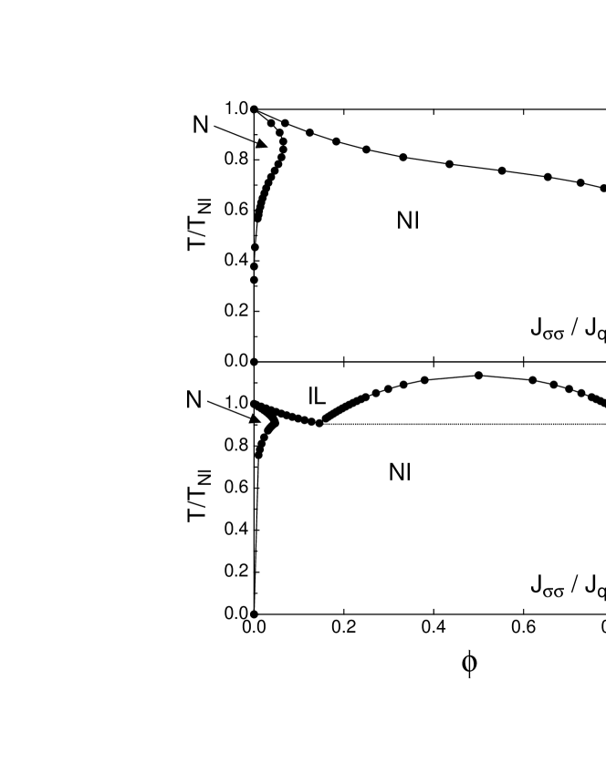
Figure 15: Theoretical phase diagram in the case of direct intermicellar attraction of strength $J_{\sigma\sigma}/J_{qq}=3/4$ (upper panel) and $J_{\sigma\sigma}/J_{qq}=3/2$ (lower panel), where the value corresponding to $\phi=0.5$ is the demixing temperature $T_{C}$ given by Eq.(34.)

The final step necessary to obtain the coexistence values $n_{N}$ and $n_{I}$ (the nematic and isotropic LC densities at coexistence respectively) is the Maxwell equal area construction. It is clear that the resulting phase diagram will be influenced by the competition between the usual pure nematic-isotropic transition (associated to the free energy Eq. (29)) and the usual lattice gas transition (whose free energy is Eq.(31)). We shall study the isotropic-nematic transition as a function of the micelle molar fraction $\phi=1-n$ and on the ratio $J_{\sigma\sigma}/J_{qq}$. The results are depicted in Figs. 14, 15 in the case $J_{\sigma\sigma}/J_{qq}=0$ (no direct micelle-micelle interaction), $J_{\sigma\sigma}/J_{qq}=3/4<1$ (weak direct micelle-micelle interaction) and $J_{\sigma\sigma}/J_{qq}=3/2>1$ (strong direct micelle-micelle interaction) respectively. The temperature axis is scaled in terms of the nematic-isotropic (NI) transition temperature $T_{NI}$ of the fully occupied counterpart (FLL), which turns out to be

$$\frac{k_{B}T_{NI}}{J_{qq}}=1.9813\ldots$$ (33)

In Fig. 14, there is no direct coupling among the micelles ($J_{qq}=0$) although there is an effective interaction as we shall see later on. As the micelles concentration $\phi$ increases, the isotropic phase (I) is depressed until it vanishes at $\phi=1$, a nematic re-entrant phase (N) appears in the small $\phi$ region, and the two phases are separated by a nematic-isotropic region (NI). In figure 15 the direct micelle-micelle coupling is weaker that the LC counterpart and the liquid-gas transition lies well inside the isotropic-nematic coexistence phase. Hence, the phase diagram is topologically similar to the previous one. At sufficiently high values of the direct coupling (Fig. 15 lower panel) the liquid-gas transition characteristic of the lattice gas model preempts the isotropic-nematic transition at intermediate micelle molar fraction. In this case, the consolution curve separating an isotropic phase with low micellar concentration (IL) from an isotropic phase with high micellar concentration (IH), is symmetric because of the vacancy/filled site symmetry, and its highest point corresponds to the liquid-gas critical temperature $T_{c}$

$$\frac{k_{B}T_{C}}{J_{qq}}=\frac{3}{2}\frac{J_{\sigma\sigma}}{J_{qq}}$$ (34)

The above phase diagram, as derived from a mean-field theory, is completely consistent with recent Monte Carlo numerical simulations on the same model pre42 , although the numerical values are not, as one expects from a mean-field-like theory such as the one treated here.

IV.1.2 Correlation Functions

In order to make a connection with the experimental results probing both the paranematic fluctuations and the micellar density fluctuations, in this Section we compute the correlation lengths. This can be done rather conveniently within our mean field theory by computing the correlation functions as follows. The micelle-micelle correlation function is defined as

$$g^{\sigma\sigma}_{xy} = \langle(1-\sigma_{x})(1-\sigma_{y})\rangle-\langle(1-\sigma_{x})\rangle\langle(1-\sigma_{y})\rangle$$ (35)

$$= \langle\sigma_{x}\sigma_{y}\rangle-\langle\sigma_{x}\rangle\langle\sigma_{y}\rangle$$ (36)

This can be easily computed in momentum space

$$g^{\sigma\sigma}_{xy}=\frac{1}{N}\sum_{\textbf{p}}e^{i\textbf{p}(\textbf{x}-\textbf{y})}\hat{g}^{\sigma\sigma}(\textbf{p})$$ (37)

as its Fourier transform displays the following very simple form

$$g^{\sigma\sigma}(\textbf{p})=\frac{1}{n^{-1}(1-n)^{-1}-2K_{\sigma\sigma}\sum^{3}_{\mu=1}\cos{p_{\mu}a}}$$ (38)

The correlation length for the micellar density $\xi_{M}$ can be immediately inferred from the behavior of $g^{\sigma\sigma}(\textbf{p})$ in the continuum limit, leading to

$$g^{\sigma\sigma}_{x,y}=\frac{1}{4\pi K_{\sigma\sigma}}\frac{e^{-|x-y|/\xi_{M}}}{3/\xi_{M}}$$ (39)

with

$$\frac{\xi_{M}}{a}=\sqrt{\frac{K_{\sigma\sigma}/9}{n^{-1}(1-n)^{-1}-6K_{\sigma\sigma}}}$$ (40)

It is worth noticing that $\xi_{M}\rightarrow 0$ as $K_{\sigma\sigma}\rightarrow 0$, meaning that, at the mean field level, there is no micelle-micelle interaction, in the absence of an explicit coupling among them. Accordingly, the above expression diverges at the (reduced) spinodal temperature $T_{S}$

$$\frac{k_{B}T_{S}}{J_{qq}}=6n(1-n)\frac{J_{\sigma\sigma}}{J_{qq}}$$ (41)

which coincides with that of a simple lattice gas model. Only going beyond the mean field approximation, as described in the next Section, a LC mediated intermicellar interaction can be described.

It is also interesting to evaluate how the micelle-LC coupling intrinsically present in this system affects the orientational pretransitional behavior. The nematic correlation function is defined as

$$G^{\alpha\beta\mu\nu}_{xy}=\langle\sigma_{x}Q_{x}^{\alpha\beta}\sigma_{y}Q_{y}^{\mu\nu}\rangle-\langle\sigma_{x}Q_{x}^{\alpha\beta}\rangle\langle\sigma_{y}Q_{y}^{\mu\nu}\rangle$$ (42)

which can be conveniently expressed in terms of the derivative of the Legendre transform of $F_{MF}$

$$[G^{\alpha\beta\mu\nu}]^{-1}=\frac{\partial^{2}}{\partial q^{\alpha\beta}_{x}\partial q_{y}^{\mu\nu}}[\beta\hat{\Gamma}_{MF}]$$ (43)

In the frame in which Eq.(22) holds, it is then easy to calculate $G_{xy}^{3333}\equiv G_{xy}$. This can be computed along the same lines as for the micellar case. One obtains, after some algebra, an expression similar to Eq.(39) with the orientational correlation length $\xi_{N}$ given by

$$\frac{\xi_{N}}{a}=\sqrt{\frac{3B(K_{qq})}{A(K_{qq},q,n)-3B(K_{qq})}}$$ (44)

where

$$A(K_{qq},q,n)=12K_{qq}\left\{1-2K_{qq}\left[\frac{9}{16}n(1-n)\Phi^{2}(\frac{27}{2}K_{qq}q)+\frac{81}{16}nR_{4}(\frac{27}{2}K_{qq}q)\right]\right\}$$ (45)

$$B(K_{qq})=2K_{qq}$$ (46)

and where we have defined the quantity

$$R_{4}(\lambda)=\frac{I_{4}(\lambda)}{I_{0}(\lambda)}-\frac{I_{2}^{2}(\lambda)}{I_{0}^{2}(\lambda)}$$ (47)

In particular in the isotropic phase $(q=0)$ this yields

$$\left.\frac{\xi_{N}}{a}\right|_{q=0}=\sqrt{\frac{1}{1-\frac{9}{5}K_{qq}n}}$$ (48)

diverging at the temperature

$$\frac{k_{B}T^{*}}{J_{qq}}=\frac{9}{5}n$$ (49)

and reducing, in the limit $n\to 1$, to the correct value of the FLL. The $T^{*}(\phi)$ line depicting the divergence temperature for the paranematic correlation length is shown in Fig. 14 as a function of the micellar density.

IV.2 High temperature expansion

As previously remarked, one important question arising from the mean-field calculation above is whether there exists an effective micelle-micelle interaction, even in the absence of a direct coupling, which is induced by the fluctuation of LC degrees of freedom. One possible indicator of this is the presence of a micelle spinodal line which signals the approach of a demixing instability, i.e. the divergence of the correlation length, and we saw that there is no spinodal line in the absence on an explicit coupling among the micelles. We attribute this to a deficiency of the mean field calculation.

To see that this is the case, we proceed as follows. First we split the original Hamiltonian Eq.(17) at zero field ($h^{\alpha\beta}=0$) in two parts

$$H\left(\{Q,\sigma\}\right) = H_{LC}\left(\{Q,\sigma\}\right)+H_{LG}\left(\{\sigma\}\right)$$ (50)

where

$$-\beta H_{LC}\left(\{Q,\sigma\}\right) = K_{qq}\sum_{\alpha\beta}\sum_{\langle xy\rangle}Q_{x}^{\alpha\beta}Q_{y}^{\beta\alpha}\sigma_{x}\sigma_{y}$$ (51)

and where the remaining term $H_{LG}\left(\{\sigma\}\right)$ is a lattice gas hamiltonian independent on the LC degrees of freedom $\{Q\left(\hat{s}\right)\}$. We then introduce an effective micelle-micelle reduced Hamiltonian $-\beta H_{eff}(\{\sigma\})$ by integrating out the LC degrees of freedom of the original Hamiltonian Eq.50

$$e^{-\beta H_{eff}\left(\{\sigma\}\right)} = e^{-\beta H_{LG}\left(\{\sigma\}\right)}\frac{\int D\hat{s}\;e^{-\beta H_{LC}\left(\{Q,\sigma\}\right)}}{\int D\hat{s}}$$ (52)

where we have defined

$$\int D\hat{s} = \int\prod_{x}d\hat{s}_{x}=\prod_{x}\int_{0}^{2\pi}d\phi_{x}\int_{-1}^{+1}d(\cos\theta_{x})$$ (53)

In the high temperature limit $T>>T_{c}$ then $K_{qq}<<1$ and thus

$$\int D\hat{s}\;\;e^{K_{qq}\sum_{\alpha\beta}\sum_{\langle xy\rangle}Q_{x}^{\alpha\beta}Q_{y}^{\beta\alpha}\sigma_{x}\sigma_{y}}=$$ (54)

$$\int D\hat{s}\left[1+K_{qq}\sum_{\alpha\beta}\sum_{\langle xy\rangle}Q_{x}^{\alpha\beta}Q_{y}^{\beta\alpha}\sigma_{x}\sigma_{y}+\frac{1}{2}K_{qq}^{2}\sum_{\alpha\beta}\sum_{\langle xy\rangle}Q_{x}^{\alpha\beta}Q_{y}^{\beta\alpha}\sigma_{x}\sigma_{y}\sum_{\mu\nu}\sum_{\langle zw\rangle}Q_{z}^{\mu\nu}Q_{w}^{\nu\mu}\sigma_{z}\sigma_{w}+\ldots\right]$$

Using the following results

$$\int d\hat{s}Q^{\alpha\beta}(\hat{s})=0$$ (55)

$$\int d\hat{s}Q^{\alpha\beta}(\hat{s})Q^{\mu\nu}(\hat{s})=-\frac{2}{5}\pi\delta^{\alpha\mu}\delta^{\mu\nu}+\frac{3}{5}\pi(\delta^{\alpha\mu}\delta^{\beta\nu}+\delta^{\alpha\nu}\delta^{\beta\mu})$$ (56)

we obtain, to first order in $K_{qq}$ and after rexponentiating the result, a new lattice gas Hamiltonian

$$-\beta H_{eff}\left(\{\sigma\}\right)=K_{\sigma\sigma}^{eff}\sum_{\langle xy\rangle}\sigma_{x}\sigma_{y}+\sum_{x}\mu^{*}(1-\sigma_{x})$$ (57)

where

$$K^{eff}_{\sigma\sigma}=K_{\sigma\sigma}+\frac{9}{40}K^{2}_{qq}$$ (58)

which amounts to an effective coupling

$$J^{eff}_{\sigma\sigma}=J_{\sigma\sigma}+\frac{9}{40}\frac{J^{2}_{qq}}{k_{B}T}$$ (59)

Notice that $J^{eff}_{\sigma\sigma}$ depends upon the temperature $T$.

In the case $K_{\sigma\sigma}=0$, we can calculate the spinodal line $T_{S}(n)$ on the basis of the mean field solution of the standard lattice gas model. We obtain

$$\frac{k_{B}T_{S}}{J_{qq}}=\sqrt{\frac{27}{20}n(1-n)}$$ (60)

which is also depicted in Fig. 14. Note that this result differes from that of a simple lattice gas (Eq. 41) because of the $T$ dependence of the effective coupling.

This analysis shows effective micelle-micelle interactions, can be computed by eliminating the LC degrees of freedom from the problem, as done here through a calculation correct to a first order in a high temperature expansion.

IV.3 Radial coupling

Before ending this section, we wish to comment on a possible additional term appearing in the general Hamiltonial (17). As described in Ref.pre6 , the properties of the present system can be strongly influenced by a directional coupling between the LC and the micelles. Hence one is tempted to include a tendency of the LC to be oriented along the radial direction of the micelles whenever the LC lie in their proximity, as a possible consequence of the tendency for homeotropic anchoring of DDAB.

To account for this we add the following additional term $-\beta\Delta H_{A}$ to the Hamiltonian in Eq.(17)

$$-\beta\Delta H_{A}=\frac{K_{q\sigma}}{a{{}^{2}}}\sum_{\alpha\beta}\sum_{\langle xy\rangle}[(1-\sigma_{x})\sigma_{y}Q_{y}^{\beta\alpha}(\textbf{y}-\textbf{x})^{\alpha}(\textbf{y}-\textbf{x})^{\beta}\\ +\sigma_{x}(1-\sigma_{y})Q_{x}^{\alpha\beta}(\textbf{x}-\textbf{y})^{\alpha}(\textbf{x}-\textbf{y})^{\beta}]$$ (61)

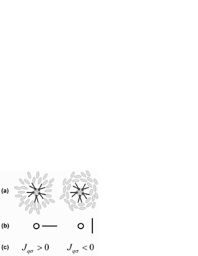
Figure 16: Possible Liquid crystal couplings at the micelle surface. Left: radial coupling. Right: tangential coupling. a: 2D pictorial view of the couplings. b: schematization of the coupling as in the lattice spin model, where circle represents an empty site and the segments the headless spins. c: coefficient $K_{q\sigma}$ of eq. 61 expressing the coupling strenght.

As described in Fig. 16, the sign of $K_{q\sigma}=\beta J_{q\sigma}$ identifies the preferred orientation of the LC with respect to its distance from the center of the neighboring the micelle. If $J_{q\sigma}>0$ the LC at the LC-micelles interface tend to align radially. It is easy to see that, at the mean field level, the above term does not affect the phase diagram. This is because mean field theory effectively eliminates the site dependence of the order parameters.

Things are different when the same coupling is investigated through high temperature expansion. In this case, the radial coupling leads to non-trivial three-body terms. This, at variance with the mean-field theory, indicates the possible relevance of the LC anchoring on the micellar surface.

V Discussion

V.1 Comparison between experimental results and theoretical model

The existence of Casimir-style, fluctuation mediated inter-micellar attractions, demonstrated by the high temperature expansion in the case of no direct coupling ($K_{\sigma\sigma}=0$), is a key result that enables us to interpret the observation of pretransitional micellar density fluctuations in systems where paranematic fluctuations are also observed. Indeed, the theoretical modelling enables us to understand the inter-micellar attraction documented in the experiments as interactions mediated by paranematic fluctuations.

More specifically, we argue that the experimental conditions we investigated correspond to $K_{\sigma\sigma}\approx 0$ and $K_{q\sigma}\approx 0$. The simultaneous presence of micellar and orientational fluctuations, and the fact that upper critical solution points have never been observed in w/o microemulsions, make us reject as unlikely (but not impossible) that a direct interaction may be at the origin of the observed behavior. Such an interaction should in fact be independent from the ordering of the solvent and of a different nature with respect to those leading to lower critical consolution point in other systems pre31 . On the other hand, the fact that the single molecule dynamics detected by EBS is unaffected by the presence of the micelles (see Section III.2.2), together with the nanosize of the droplet radius, way shorter than typical extrapolation lengths for surface anchoring, strongly support the notion that the 5CB anchoring at the micellar surface is very weak.

Therefore, we read the observed increase in $\langle I_{M}\rangle$ and decrease in $D_{M}/D_{0}$ on the basis of the theoretical predictions that the softening of the micellar system (increase of micellar osmotic compressibility and associated slowing down) is expected on the only basis of the micellar dilution effect of the local nematic matrix. The existence of a bell-shaped spinodal curve in Fig. 14, suggests that a similar curve could be present in the experimental phase diagram as well (Fig. 2), although hidden into the coexistence region. Thus, on lowering T, i.e. on approaching the spinodal line increasing micellar density fluctuation are expected. Accordingly, we have fitted $\langle I_{M}\rangle$ vs. $T$ with $(T-T_{S})^{-1}$. The extracted values for $T_{S}(\phi)$, which suffer of a rather large indetermination because of the intrinsically limited range of the fit, are shown in Fig. 2. The two data point appear to decrease with increasing $\phi$ for $\phi>0.075$, but for small experimentally inaccessible $\phi$, $T_{S}(\phi)$ must take a positive slope since the system of highly diluted micelles necessarily approaches gas-like non-interacting behavior.

The comparison between the experimental phase diagram (Fig. 2) and the theoretical one (Fig.14) enlightens a remarkable similarity in all the qualitative features: re-entrant nematic phase, shape of the coexistence curve, non-trivial divergence lines determining the orientational and micellar pretransitional fluctuations. However, no quantitative comparison can be drawn between the two phase diagrams because of the approximations at the base of the model and in the techniques used to solve it. Both the temperature and the micellar density axes cannot be easily mapped on the corresponding experimental quantities. For example, the $T_{NI}-T^{*}$ gap for the pure nematic as well as the value of $\phi$ corresponding to the maximum in the spinodal curve are both much larger than the corresponding observed quantities. These shortcomings are consequences, respectively, of the intrinsic limitations of the mean field approximation and of having assumed that micelles and LC molecules have equal volumes .

According to the interpretation here proposed, the expulsion of micelles by orientational ordering, explicitly manifested at low T in the macroscopic phase separation, is at the root of the whole phase behavior of $5DH\mu em$. Nematic correlations appear more easily where the local micelle concentration is lower, and in turn force out micelles, thus further reducing the local amount of annealed disorder and increasing the local $T^{*}$, with the consequent increase of local nematic order. Theoretical considerations indicate that sufficiently small impurities incorporated in the nematic phase display attractive long ranged interactions due to orientational fluctuations of the LC pre50 . This is a consequence of the impurity induced depression of the local nematic order which are thus segregated to minimize the total free energy, a mechanism that bears some resemblance to the prewetting induced colloidal aggregation pre51 , or to the depletion forces in critical systems pre52 . We argue that the same mechanism should be present in the isotropic phase but with an exponential cut-off at $\xi_{N}$. This notion is corroborated by the experimental coincidence between the average intermicellar distance d and the maximum value of $\xi_{N,max}=\xi_{0}[T^{*}/(T_{DM}-T^{*})]^{\frac{1}{2}}$, with $\xi_{0}\sim 10\mbox{\AA}$ : for $\phi=0.075$, $\xi_{N,max}\sim 95\mbox{\AA}$, $d\sim 58\mbox{\AA}$; for $\phi=0.15$, $\xi_{N,max}\sim 75\mbox{\AA}$, $d\sim 74\mbox{\AA}$).

V.2 Concentration dependence of the transition temperatures

All the observed $5DH\mu em$ behavior appears determined by three relevant temperatures: the demixing temperature $T_{DM}(\phi)$, the divergence temperature for paranematic fluctuations $T^{*}(\phi)$, the spinodal temperature $T_{S}(\phi)$. We want here discuss the origin of their $\phi$ dependence.

One of the most striking features of the phase diagram of the $5DH\mu em$ is the high negative slope of $T_{DM}(\phi)$ and $T^{*}(\phi)$: $T_{NI}-T_{DM}(\phi)\sim 4.4K$ and $T_{NI}-T^{*}(\phi)\sim 7K$ for the $5DH\mu em$ $\phi=7.5\%$; $T_{NI}-T_{DM}(\phi)\sim 7.6K$ and $T_{NI}-T^{*}(\phi)\sim 11K$ for the $5DH\mu em$ $\phi=15\%$. Thus $dT_{DM}(\phi)/d\phi\sim-60K$ and $dT^{*}(\phi)/d\phi\sim-80K$. These numbers are quite larger than the T shift in the position of the specific heat $(c_{p})$ peak observed by studying LC with nanosized quenched disorder: $dT_{NI}(\phi)/d\phi\sim-7.1K$ for 8CB embedded in silica aerogel pre36 and $dT_{NI}(\phi)/d\phi\sim-8.2K$ for $8CB$ incorporating soft gels of aerosil particles pre37 . The origin of such a difference will also be discussed in the following.

V.2.1 Demixing temperature $(T_{DM})$

The determination of the presence and size of the droplets enables us to better discuss the low concentration part of the phase diagram. Indeed, the value of $\beta_{I}$, too low if calculated on the basis of the molar fraction of monomeric DDAB (see Section III.A), takes a much higher value when referred to the molar fraction of micellar aggregates, which can be calculated from the mass of a single micelle. The radius that micelles would have if DDAB were compacted in a sphere was estimated to be about $13.5\mbox{\AA}$ (see Sec. III.C.3). Based on this value, the slopes of the isotropic and nematic phase boundary vs. contaminant fraction are, respectively $\beta_{I}\sim-4.17$ and $\beta_{N}\sim-31.85$. We thus obtain $(\beta_{N}^{-1}-\beta_{I}^{-1})\sim 0.21$, in a much better agreement with the prediction of $(\beta_{N}^{-1}-\beta_{I}^{-1})\sim 0.25$. The numerical difference between the two numbers indicates that the calculation partially underestimates the slope of the isotropic phase boundary.

The same relationship between phase boundary and contaminant concentration can be reformulated under a different prospective, which offers a better insight on its physical basis. By approximating $\beta_{N}^{-1}\sim 0$, the occurrence of the $5DH\mu em$ demixing transition coincides with a transformation of a fraction of the LC from isotropic to nematic and, at the same time, with the segregation of the inverted micelles in the isotropic phase. By balancing the gain in free energy density for the nematic ordering of 5CB $(\Delta G_{NI}(T))$ against the work done against the osmotic pressure $\Pi$ of the micelles, we obtain

$$\Delta G_{NI}(T)=\Pi(\phi)$$ (62)

$\Delta G_{NI}(T)$ can be computed on the basis of the Landau-deGennes expansion, whose coefficients for bulk 5CB have been determined pre53 . Indeed, since the micelle-disordered isotropic cannot differ much from the unperturbed isotropic (especially because surface coupling is very weak), and since the nematic phase in the $5DH\mu em$ is almost micelle-free, $\Delta G_{NI}(T)$ calculated for bulk 5CB is a good approximation for the difference in free energy between nematic micelle poor phase and isotropic micelle rich one. The osmotic pressure, on the other side, can be calculated on the basis of $\phi$ and R, the micellar radius, and by assuming a perfect gas behavior. With this with these ingredients, it is possible to extract $\beta_{I}$ in the limit of small $\phi$ . With this crude estimate we obtain $\beta_{I}\sim-6.5$. Although overestimating the measured $\beta_{I}$, this figure is close enough to the data to indicate that indeed the temperature depression of the demixing transition can be understood as a direct consequence of the very nature of the demixing. This fact once again confirms the appropriateness of describing the $5DH\mu em$ as a pseudo-single component system.

V.2.2 Paranematic divergence temperature $(T^{*})$

According to the model $T^{*}(\phi)=T^{*}(\phi=0)\cdot(1-\phi)$ (see Section IV). The decrease of $T^{*}$ with $\phi$ can be easily interpreted as a dilution effect on the coupling strength. Indeed, the dilution brings about a decrement in the average coordination number of each spin. As a consequence $\overline{J_{qq}}$, the coupling coefficient averaged on all bonds, also decreases. Since $\phi$ is the probability to find a micelles as nearest neighbor of each given spin, $\overline{J_{qq}}=J_{qq}\cdot(1-\phi)$. Hence, it appears that the easiest interpretation of the observed $T^{*}(\phi)$ is to picture it as a direct consequence of a dilution induced weakening of the molecular field, which, in the experimental case, is associated to the presence of interfaces reducing the coordination number of the 5CB molecules. A possible estimate of the fraction of 5CB molecules at contact with the micellar surface is given by the volume between $13.5\mbox{\AA}$ and $20\mbox{\AA}$ from the center of the micelle, i.e. by the difference between the volume hydrodynamically attached to the micelle and the total water-DDAB volume. This would imply that a fraction of about $f=3.2\cdot\phi$ of the total 5CB molecules experience reduced coordination because of the proximity of DDAB molecules. Comparing $T^{*}(\phi)=T^{*}(\phi=0)\times(1-\phi)$ with the experimentally observed $dT^{*}(\phi)/d\phi\sim-80K$, suggests that the coordination number of 5CB molecules at the DDAB interface is reduced of 8 %. This number appears reasonable, since we expect it to be lower than the simplest available analogy of a hard sphere crystal limited by a plane. In that case spheres facing the plane have a coordination of 9 while in the bulk the coordination is 12, yielding a decrease of $25\%$ of the coordination number. This simple evaluation, despite its extreme roughness, supports the notion that the concentration dependence of $T^{*}$, and thus the whole T downshift in the pretransitional paranematic behavior, is due to dilution induced weakening of the intermolecular coupling.

V.2.3 Comparison with LC in silica gels

The N-I transition in LC with dispersed silica nanostructures, either aerogel or aerosil, displays a specific heat $c_{p}$ peak downshifted in T with respect to the corresponding transition in the bulk and downshifted in T. In those systems it is found that the whole paranematic behavior is unmodified but ”rigidely” shifted in temperature (pre36 , pre37 ). It is quite remarkable that such observed $dT^{*}/d\phi$ in the aerogel/aerosil LC systems is about ten times smaller than in $5DH\mu em$. The different nature of the disordering provided by the two structures hosted in the LC, mobile ”annealed” disorder in $5DH\mu em$ and static ”quenched” disorder in nanosilica-LC materials, cannot be the origin of this large effect. This is because the different degrees of freedom are highly mobile in the high temperature phase, thus preventing a clear distinction between a frozen impurity and an equilibrated one.

The difference between the two systems can, at least in part, be understood on the basis of different dilution induced weakening of intermolecular coupling, along the line of the discussion in the previous section. X-ray characterization of the empty aerogel structure - not available in the aerosil case - enable extracting the specific interface extension of the structures, expressed in the S/V ratio, where S is the silica surface area and V the aerogel volume pre54 . For a particular family of silica aerogel extensively characterized in the past, it is found that, approximately, $S/V=0.11\mbox{\AA}^{-1}$ pre38 . It follows that the fraction of LC molecules at the silica interface is approximately $f\sim S/V\cdot\sqrt[3]{v_{LC}}\sim 0.8$ , where $v_{LC}$ is the volume of a single LC molecule. Thus, at equal volume fraction, the silica aerogel is characterized by an interface about three times smaller than the $5DH\mu em$, which would imply a value of $dT^{*}/d\phi$ three times smaller, thus only in part accounting for the experimentally observed difference. This fact indicates that some other factor plays a relevant role in determining the $T^{*}$ shift, possibly related either to the different surface coupling of the two surfaces or to the different geometry of the disordering hosts: well dispersed in the $5DH\mu em$, while necessarily interconnected in the aerogel.

VI Conclusions

In this article we have presented a systematic investigation of a system where thermodynamically stable nanoparticles are dispersed in a thermotropic liquid crystal. As it appears from the experiments, the self aggregated nature of the particles does not play any observable role, in agreement with the notion that such self assembly is governed by forces larger than the molecular field strength provided by nematic ordering. This system enables studying the effect of annealed disorder on the phase diagram of the liquid crystal, and, at the same time, thanks to the large optical contrast provided by the droplets’ water core, it also allows direct observation of the statistical properties of the dispersed nanoparticles.

We found that the system exhibits a phase transition combining the demixing of the nano-droplets with nematic ordering in one of the coexisting phases. The phase diagram also features an intriguing reentrant nematic phase. This feature indicates a temperature dependent solubility of nano-droplets in the nematic phase.

The characteristic frequency of the electric birefringence spectra expressing the time to redirect the molecular axis, shows that the dispersed nanoparticles do not alter appreciably the local molecular environment which remains bulk-like. This fact supports the notion that, mostly because of their nano-size, microemulsion droplets do not provide significant anchoring on the neighboring LC molecules. Hence, the observed effects of the nanoinpurities on the IN phase transition have to be understood simply as consequences of dilution, in strong analogy with the most conventional understanding of the effects of molecular contaminants. Along this line we have here presented a theoretical analysis aimed to determine the phase behavior of a diluted Lebwohl-Lasher spin lattice model, where LC molecules are mimicked by pointless spin vectors on a cubic lattice and micelles are vacancies on the same lattice. The spin variables interact via a Maier-Saupe orientational coupling, provided that nearest neighbour pairs are occupied by LC variables. This system has been solved by mean-field theory and high-temperature expansion.

Experimental observations and theoretical predictions nicely match offering a simple ground to interpret all the basic features of the system.

The rather complex topology of the observed phase diagram (demixing transition and re-entrant nematic phase) simply follows from the tendency of liquid crystal towards orientational order with no need for either micelle-micelle or micelle-LC direct interactions. The dependence of phase boundaries and divergence temperatures on the concentration of impurities conveys the mutual effects of orientational order and nanoparticle dispersion. Furthermore, the study of the light scattered by the nanodroplets in the isotropic phase close to the $IN$ transition, enlightens the presence of intermicellar attractive forces which the theoretical model enables interpreting as a consequence of the paranematic orientational fluctuations. This can be seen by eliminating the LC variables in the Hamiltonian of the spin model, approximated to the leading order in a high temperature expansion. An effective temperature dependent micelle-micelle interaction is found, whose strength depends on the orientational coupling between the LC molecules. This fluctuation mediated interaction is intrinsic to the very presence of nanoimpurities, necessarily diluting the LC, while the addition of possible surface anchoring does not change the picture within a mean-field theory, but has a non-trivial effect within our high-temperature expansion. Accordingly, it appears interesting to explore how the phase diagram is modified by increasing the droplet size and the hydrophobic portion of the surfactants, which should lead to progressively stronger anchoring.

We acknowledge support from NATO (Collaborative Linkage Grant) and from MIUR (PRIN 2004024508)

Figure 14: Theoretical phase diagram calculated in the case of no direct intermicellar interaction $J_{\sigma\sigma}=0$. The temperature axis is scaled with the nematic-isotropic transition temperature $T_{NI}$ of the fully occupied model (see Eq.(33)). The dotted line is the spinodal line $T_{S}$ for micellar demixing, obtained through a high temperature expansion, Eq.(60). The dashed line corresponds to the divergence temperature $T^{*}$ for the nematic correlation length, Eq.(49).

References

- (1) Liquid Crystals in Complex Geometries, edited by G.P. Crawford and S. Zumer (Taylor & Francis, London, 1996)
- (2) S.Elston and R.Sambles, The optics of thermtropic liquid crystals (Taylor & Francis, London 1998)
- (3) T. Bellini, N.A. Clark, C.D. Muzny, L. Wu, C.Garland, D.W. Schaefer and B.J. Oliver, Phys. Rev. Lett. 69, 788 (1992)
- (4) T. Bellini, L. Radzihovsky, J. Toner and N.A. Clark, Science 294, 1074 (2001)
- (5) P. Poulin, H. Stark, T.C. Lubensky & D.A. Weitz, Science 275, 1770 (1997)
- (6) M.A. Marcus, Mol. Cryst. Liq. Cryst. 110, 145 (1984)
- (7) J. Yamamoto & H. Tanaka, Nature 409, 321-325 (2001)
- (8) T. Bellini, M. Caggioni, N.A. Clark, F. Mantegazza, A. Maritan, A. Pelizzola, Phys. Rev. Lett. 91, 085704 (2003)
- (9) J.C. Loudet, P. Barois and P. Poulin, Nature 407, 611 (2000)
- (10) C. Shen and T. Kyu, J. Chem. Phys. 102, 556 (1995)
- (11) G.A. Oweimreen and D.E. Martire, J. Chem. Phys. 72, 2500 (1980)
- (12) J. Corcoran, S. Fuller, A. Rahman, N. Shinde, G.J.T. Tiddy, G.S. Attard, J. Mater. Chem. 2, 695 (1992)
- (13) B. Pouligny, J.P. Marcerou, J.R. Lalanne and H.J. Coles, Mol. Phys. 49, 583 (1983)
- (14) D. Lippens, J.P. Parneix and A. Chapoton, J. Physique 38, 1465 (1977)
- (15) A. Hourri, P. Jamee, T.K. Bose and J. Thien, Liq. Cryst. 29, 459 (2002)
- (16) T.K. Bose, B. Campbell, S. Yagihara and J. Thoen, Phys. Rev. E 36, 5767 (1987)
- (17) M. Caggioni, F. Mantegazza, T. Bellini, to be published
- (18) S. Urban, B. Gestblom and R. Dabrowski, Phys. Chem. Chem. Phys. 1, 4843 (1999)
- (19) W.H. De Jeu, Liquid crystals, edited by L.Liebert, Solid State Physics, supplement 14 (Accademic Press New York 1978)
- (20) J. Jadzyn, R. Dabrowsky, T. Lech and G. Czechowski, J. Chem. Eng. Data 46, 110 (2001)
- (21) H. Herba, A. Szymanski and A. Drzymala, Mol. Cryst. Liq. Cryst. 127, 153 (1985)
- (22) G.W. Gray, K.J. Harrison, J.A. Nash, J. Constant, D.S. Hulme, J. Kirton, E.P. Raynes, Liq. Cryst. Ordered Fluids 2, 617 (1974)
- (23) T.W. Stinson, J.D. Litster and N.A. Clark, J. Physique, Coll. C1 33, 69 (1972)
- (24) P.G. de Gennes and J. Prost, The Physics of Liquid Crystals (Claredon Press, Oxford 1993)
- (25) P.A. Egelstaff, An Introduction to The Liquid State (Claredon Press, Oxford, 1994)
- (26) M. Corti and V. Degiorgio, J. Chem. Phys. 85, 711 (1981)
- (27) A.M. Cazabat and D. Langevin, J. Chem. Phys. 74, 3148 (1981)
- (28) D.J. Cebula, R.H. Ottewill, J. Ralston and P.N. Pusey, J. Chem. Soc. Faraday Trans. I 77, 2585 (1981)
- (29) R. Finsy, A. Devriese and H. Lekkerkerker, J. Chem. Soc. Faraday Trans. II 76, 767 (1980)
- (30) M.W. Kim, W.D. Dozier and R. Klein, J. Chem. Phys. 84, 5919 (1986)
- (31) J. Ricka, M. Borkovec, U. Hofmeier and H.F. Eicke, Europhys. Lett 11, 379 (1990)
- (32) J.S. Huang and M.W. Kim, Phys. Rev. Lett. 47, 1462 (1981)
- (33) J.S. Huang, S.A. Safran, M.W. Kim, and G.S. Grest, Phys. Rev. Lett. 53, 592 (1984)
- (34) S.J. Chen, D.F. Evans, B.W. Ninham, D.J. Mitchell, F.D. Blum, S. Pickup, J. Phys. Chem. 90, 842 (1986)
- (35) M. Monduzzi, F. Caboi, F. Larche and U. Olsson, Langmuir 13, 2184 (1997)
- (36) M. Olla and M. Monduzzi, Langmuir 16, 6141 (2000)
- (37) H.C. van de Hulst, Light Scattering by Small Particles (Dover Publications, New York, 1981)
- (38) P. Lebwohl and G. Lasher, Phys. Rev. A 6, 426 (1972)
- (39) A. Maritan, M. Cieplak, T. Bellini and J. R. Banavar, Phys. Rev. Lett 72, 4113 (1994)
- (40) T. Bellini, M. Buscaglia, C. Chiccoli, F. Mantegazza, P. Pasini and C. Zannoni, Phys. Rev. Lett. 85, 1008 (2000)
- (41) W. Maier and A. Saupe, Z. Naturf. A 13, 564 (1958)
- (42) R.L. Humphries and G.R. Luckhurst, Proc. R. Soc. Lond. A 352, 41 (1976)
- (43) R. Hashim, G.R.Luckhurst and S. Romano, Proc. R. Soc. London A 429, 323 (1990) and references therein
- (44) Advances in the Computer Simulation of Liquid Crystals, P. Pasini and C. Zannoni (Eds) 99-117 (Kluwer, Dordrecht, 2000)
- (45) U.Fabbri and C. Zannoni, Mol. Phys. 58, 763 (1986)
- (46) M. A. Bates, Phys. Rev. E 64, 051702 (2001)
- (47) A. Matsuyama and T. Kato, Phys. Rev. E 59, 763 (1999)
- (48) D. Bartolo, D. Long and J.-B. Fournier, Europhys. Lett. 49, 729 (2000)
- (49) D. Beysens and D. Esteve, Phys. Rev. Lett. 54, 2123 (1985)
- (50) R. Piazza and G. Di Pietro, Europhys. Lett. 28, 445 (1994)
- (51) L. Wu, B. Zhou, C. W. Garland, T. Bellini, and D. W. Schaefer, Phys. Rev. E 51, 2157 (1995)
- (52) G. S. Iannacchione, C. W. Garland, J. T. Mang and T. P. Rieker, Phys. Rev. E 58, 5966 (1998)
- (53) H. J. Coles, Mol. Cryst. Liq. Cryst. 49, 67 (1978)
- (54) A. Emmerling and J. Fricke, J. Non-Cryst. Solids 145, 113 (1992)
- (55) A.G. Rappaport, N.A. Clark, B.N. Thomas and T. Bellini, chapter 20 of Ref. 1.