Magnetic quantum oscillations in nanowires

Abstract

Analytical expressions for the magnetization and the longitudinal conductivity of nanowires are derived in a magnetic field, $B$. We show that the interplay between size and magnetic field energy-level quantizations manifests itself through novel magnetic quantum oscillations in metallic nanowires. There are three characteristic frequencies of de Haas-van Alphen (dHvA) and Shubnikov-de Haas (SdH) oscillations, $F=F_{0}/(1+\gamma)^{3/2}$, and $F^{\pm}=2F_{0}/|1+\gamma\pm(1+\gamma)^{1/2}|$, in contrast with a single frequency $F_{0}=S_{F}\hbar c/(2\pi e)$ in simple bulk metals. The amplitude of oscillations is strongly enhanced in some ”magic” magnetic fields. The wire cross-section area $S$ can be measured using the oscillations as $S=4\pi^{2}S_{F}\hbar^{2}c^{2}/(\gamma e^{2}B^{2})$ along with the Fermi surface cross-section area, $S_{F}$.

High magnetic fields have been widely used to explore the single particle spectrum of bulk metals. Historically, dHvA and SdH quantum oscillations in magnetic fields have provided an unambiguous signature and accurate quantitative information on the Fermi surface and the damping of quasiparticles shon . Essential deviations from the conventional three-dimensional (3D) oscillations have been found in low-dimensional metals like 2D organic conductors sin ; kar . At present conducting nanowires and nanotubes of almost any cross-section down to nanometer scale and of any length can be prepared with modern nano-technologies aledem . There are significant opportunities for discovery of unique nanoscale phenomena arising from the dimension quantization. In particular, galvanomagnetic transport properties of nanowires have been the subject of many studies during last decades her . Heremas et al. her observed the semimetal-semiconductor phase transition in the magnetoresistance caused by the interplay between the electron cyclotron orbits, the size energy-level quantization and the inter-band transfer of carriers in Bi nanowires. Their magneto-conductance was theoretically addressed in the extreme 1D limit sinmol . The Aharonov-Bohm-type oscillations of the magneto-conductance have been discovered in carbon nanotubes bac ; fuj and connected with a metal-insulator transition caused by shifting of the van Hove singularities of the density of states roc . More recently SdH oscillations were observed in arrays of 80 nm Bi-nanowires hub and in 200nm Bi-nanowires gro in first and second derivatives of resistance with respect to the magnetic field. There is a great demand for quantitative characterization of nanowires and analytical descriptions of the interplay between dimension and field-induced energy-level quantizations.

In this Letter, we present the theory of magnetic quantum oscillations in long metallic nanowires in the longitudinal magnetic field, ${\bf B}$, parallel to the direction of the wire $z$. We consider clean nanowires with the electron mean free path, $l=v_{F}\tau$ comparable or larger than the cross size, $R$, but smaller than the nanowire length, $L$, which allows us to apply the conventional Boltzmann kinetics. We also assume that the electron wavelength near the Fermi level is very small in the metallic nanowires, so that $L\gg l\gtrsim R\gg 2\pi\hbar/(m^{*}v_{F})$, where $v_{F}$ is the Fermi velocity and $m^{*}$ is the band mass in the bulk metal. We find novel quantum oscillations of the magnetization and the conductivity caused by the interplay between magnetic and dimension energy-level quantizations.

Let us first calculate the magnetization $M=-\partial\Omega/\partial B$, where $\Omega=-k_{B}T\sum_{\alpha}\ln[1+\exp(-\xi_{\alpha}/(k_{B}T))]$ is the thermodynamic potential, $\xi_{\alpha}=E_{\alpha}-\mu$, $E_{\alpha}$ is the single-particle energy spectrum and $\mu$ is the chemical potential.

Boundary conditions on the surface of the wire are not compatible with the symmetry of the vector potential, ${\bf A}={\bf B}\times{\bf r}/2$, so there are no simple analytical solution for $E_{\alpha}$ in the magnetic field. However, one can overcome this difficulty in the quasi-classical limit, $\mu\gg\hbar\omega_{s}$, where $\omega_{s}\equiv\pi v_{F}/R$, using the Tomonaga-like linearization of the energy spectrum tom . Approximating the wire as an infinite round well one obtains $E_{\alpha}=\hbar^{2}(k_{nm}^{2}+k^{2})/(2m^{*})$. Here $\hbar k$ is the continuous momentum along the wire, and discrete $k_{nm}$ are defined as zeros of the Bessel functions $J_{|m|}(k_{nm}R)=0$, where $m=0,\pm 1,\pm 2,...$ are the eigenvalues of z-component of the orbital momentum. In the quasi-classical limit $J_{|m|}(k_{nm}R)\approx(k_{nm}R)^{-1/2}\cos(k_{nm}R-\pi|m|/2-\pi/4)$, and $k_{nm}R=\pi(2n+1)/2+\pi|m|/2+\pi/4$ with $n=0,1,2,...$.

Hence, near the Fermi surface the spectrum is given by $\xi_{n,m,k}\approx\hbar\omega_{s}(2n+|m|-n_{F})+\hbar^{2}k^{2}/(2m^{*})$, which is identical to the spectrum in a parabolic ”confinement” potential $V({\bf r})=m^{*}\omega_{s}^{2}(x^{2}+y^{2})/2$ (here $n_{F}=\mu/(\hbar\omega_{s})\gg 1$). The major contribution to dHvA and SdH oscillations arises from the energy spectrum near the Fermi level, so we can replace the metallic nanowire with the confinement potential. In contrast with the original problem, the model Hamiltonian, $H=({\bf p}-e{\bf A}/c)^{2}/(2m^{*})+V({\bf r})+s\mu_{B}B$ has simple analytical eigenfunctions, $\psi_{\alpha}({\bf r})\propto\exp(ikz)\rho^{|m|}\exp(-\rho^{2}/2)L_{n}^{|m|}(\rho^{2})$ and eigenvalues

$$E_{\alpha}={\hbar^{2}k^{2}\over{2m^{*}}}+2\hbar\omega\left(n+{|m|-m+1\over{2}}\right)+m\hbar\omega^{-}+s\mu_{B}B,$$ (1)

where $\rho^{2}=(m^{*}\omega/\hbar)(x^{2}+y^{2})$, $\omega^{2}=\omega_{s}^{2}+\omega_{c}^{2}/4$, $\omega^{\pm}=\omega\pm\omega_{c}/2$, $\omega_{c}=eB/m^{*}c$, $\mu_{B}$ is the Bohr magneton, and $\alpha=\{n,m,k,s\}$ comprises all quantum numbers including the spin $s=\pm 1$. Using Eq.(1) and replacing negative $m$ with $-m-1$ one obtains

$$\Omega=-k_{B}TL\sum_{s,\pm}\int{dk\over{2\pi}}\sum_{n,m\geqslant 0}\ln\left[1+\exp\left({\mu_{s}^{\pm}-\epsilon_{nm}^{\pm}(k)\over{k_{B}T}}\right)\right],$$ (2)

where $\mu_{s}^{+}=\mu-\hbar\omega-\mu_{B}Bs$, $\mu_{s}^{-}=\mu-\hbar(\omega+\omega^{+})-\mu_{B}Bs$, and $\epsilon_{nm}^{\pm}(k)=2\hbar n\omega+\hbar m\omega^{\pm}+\hbar^{2}k^{2}/(2m^{*})$. Summations over $n$ and $m$ can be replaced by sums over $r,r^{\prime}=0,\pm 1,\pm 2,....\pm\infty$ using twice the Poisson’s formula and the variables $x=2\omega n+\omega^{\pm}m$ and $y=\omega n-\omega^{\pm}m/2$ in place of $n$ and $m$,

$$\sum_{n,m\geqslant 0}f(2\omega n+\omega^{\pm}m)=\sum_{r,r^{\prime}}{1\over{2\pi i(r\omega^{\pm}-2\omega r^{\prime})}}\times$$ (3)

$$\int_{0}^{\infty}dxf(x)\left[\exp\left({2\pi irx\over{2\omega}}\right)-\exp\left({2\pi ir^{\prime}x\over{\omega^{\pm}}}\right)\right].$$ (4)

We are interested in an oscillatory correction, $\tilde{\Omega}$ to the thermodynamic potential arising from the terms in Eq.(3) with nonzero $r$ or $r^{\prime}$. Introducing a new variable $\xi=x+\hbar^{2}k^{2}/(2m^{*})-\mu_{s}^{\pm}$, integrating by parts, extending the lower limit of $\xi$ down to $-\infty$ and taking routine integrals over $k$, $\int dk\exp(iak^{2})=(\pi/|a|)^{1/2}\exp[i\pi a/(4|a|)]$ and over $y=\xi/(k_{B}T)$, $\int dy\exp(iay)[1+\exp(y)]^{-1}=-i\pi/\sinh(\pi a)$, we finally obtain

$$\tilde{\Omega}=\sum_{r=1}^{\infty}\sum_{\pm}A_{r}(\omega,\omega^{\pm})\sin\left({\pi r\mu\over{\hbar\omega}}-{\pi r(\omega^{+}\mp\omega^{-})\over{2\omega}}-{\pi\over{4}}\right)$$ (5)

$$+ A_{r}(\omega^{\pm}/2,2\omega)\sin\left({2\pi r\mu\over{\hbar\omega^{\pm}}}\pm{\pi r(\omega^{+}\mp\omega^{-})\over{\omega^{\pm}}}-{\pi\over{4}}\right),$$ (6)

where

$$A_{r}(x,y)={k_{B}TL(2m^{*}x/\hbar)^{1/2}\cos[\pi r\mu_{B}B/(\hbar x)]\over{2\pi r^{3/2}\sinh[\pi^{2}k_{B}Tr/(\hbar x)]}}\cot\left({\pi ry\over{2x}}\right)$$ (7)

are oscillation amplitudes, and the summation formula $\sum_{r}(z-r)^{-1}=\pi\cot(\pi z)$ has been applied.

Here and further we neglect quantum oscillations of the chemical potential. For the sake of transparency, we also neglect a damping of quantum levels by the impurity scattering in dHvA oscillations. We introduce this damping in the SdH effect (see below) neglecting quantum oscillations of the scattering rate $1/\tau$. The quantum oscillations of $\mu$ and $1/\tau$ could lead to a mixing of dHvA frequencies in multi-band metals as predicted and experimentally observed in several bulk compounds alebra ; sin2 ; shep ; yos . However, they are negligible in the presence of a field and size-independent ”reservoir” of states (i.e. a sub-band with a heavy mass alebra2 ) and the inter-band scattering.

There are three characteristic frequencies $2\omega$ and $\omega^{\pm}$ in the oscillating part of the magnetization $\cal{M}$ $=-\partial\tilde{\Omega}/\partial B$, rather then a single frequency $\omega_{c}$.

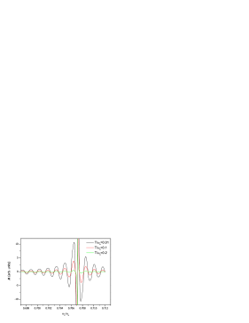
Figure 1: Oscillating part of the magnetization versus the magnetic field for relatively low fields and three temperatures. The resonance at $\omega_{c}=\omega_{s}/\sqrt{2}$ is due to a partial recovery of the energy-level degeneracy.

The same frequencies are found in the conductance, $\sigma$. The longitudinal conductivity is given by agd

$$\sigma({\bf r},\nu_{0})={ie^{2}\hbar^{2}k_{B}T\over{2\nu_{0}(m^{*})^{2}}}\sum_{s,\omega_{p}}\left({\partial\over{\partial z}}-{\partial\over{\partial z^{\prime}}}\right)_{{\bf r^{\prime}}\rightarrow{\bf r}}\times$$

$$\int d{\bf r^{\prime\prime}}\overline{G_{s}({\bf r},{\bf r^{\prime\prime}};\omega_{p}){\partial\over{\partial z^{\prime\prime}}}G_{s}({\bf r^{\prime\prime}},{\bf r^{\prime}};\omega_{p}-\nu_{0})}$$

$$- {ie^{2}k_{B}T\over{\nu_{0}m^{*}}}\sum_{s,\omega_{p}}\overline{G_{s}({\bf r},{\bf r};\omega_{p})},$$

where $\hbar\omega_{p}=\pi k_{B}T(2p+1)$, $p=0,\pm 1,\pm 2,...$, and $\nu_{0}=2\pi nk_{B}T/\hbar$ is the ”frequency” of the ”time”-dependent z-component of the vector potential, $A_{z}=iEc\nu_{0}^{-1}\exp(-i\nu_{0}t)$, due to a longitudinal electric field $E$( $0\leqslant t\leqslant\hbar/(k_{B}T)$). The static conductivity is calculated as the analytical continuation of this equation to $\nu=i\nu_{0}\rightarrow 0$. The product of two GFs averaged over the random impurity distribution is factorized as the product of averaged GFs for a short-range scattering potential in absence of vertex corrections agd ,

$$\overline{G_{s}({\bf r},{\bf r^{\prime}};\omega_{p})}=\sum_{n,m,k}{\psi_{\alpha}({\bf r})\psi^{*}_{\alpha}({\bf r^{\prime}})\over{i\hbar\tilde{\omega_{p}}-\xi_{\alpha}}},$$

where $\tilde{\omega_{p}}=\omega_{p}+\omega_{p}/(2|\omega_{p}|\tau)$. Then integrating the conductivity $\sigma({\bf r},\nu_{0})$ over the cross-section of the wire one obtains the conductance,

$$\sigma(\nu) = -{ie^{2}k_{B}T\over{L\nu_{0}m^{*}}}\sum_{\alpha,\omega_{p}}{\hbar^{2}k^{2}/m^{*}\over{(i\hbar\tilde{\omega_{p}}-\xi_{\alpha})[i\hbar(\tilde{\omega_{p}}-\nu_{0})-\xi_{\alpha}]}}$$ (10)

$$+ {1\over{i\hbar\tilde{\omega_{p}}-\xi_{\alpha}}}.$$ (11)

Integrating by parts the second diamagnetic term in Eq.(6) cancels the paramagnetic part at $\nu_{0}=0$. The routine analytical continuation lif of the remaining paramagnetic part yields the static conductance ref in the limit $\nu\rightarrow 0$,

$$\sigma=-{e^{2}\hbar^{3}\over{L\pi(m^{*})^{2}}}\sum_{\alpha}k^{2}\int_{-\infty}^{\infty}d\xi{\partial f(\xi)\over{\partial\xi}}\left[\Im G^{R}_{\alpha}(\xi)\right]^{2},$$ (12)

where $G^{R}_{\alpha}(\xi)=[\xi-\xi_{\alpha}-i\hbar/(2\tau)]^{-1}$ is the retarded GF and $f(\xi)=[1+\exp\xi/(k_{B}T)]^{-1}$.

Summations over $n$ and $m$ are performed using twice the Poisson’s formula, as in Eq.(3). The term with $r=r^{\prime}=0$ yields the classical contribution,

$$\sigma_{0}=\sum_{s,\pm}{e^{2}\tau\over{4\hbar^{3}\pi\omega\omega^{\pm}(m^{*})^{1/2}}}\int_{0}^{\infty}dxx\times$$ (13)

$${[\mu^{\pm}_{s}-x+((\mu^{\pm}_{s}-x)^{2}+\hbar^{2}/(4\tau^{2}))^{1/2}]^{3/2}\over{((\mu^{\pm}_{s}-x)^{2}+\hbar^{2}/(4\tau^{2}))^{1/2}}}$$ (14)

after integrating over $k$ and neglecting temperature corrections. One can also neglect $\hbar^{2}/(4\tau^{2})$ in the integral, Eq.(8) and obtain the conventional Drude conductance, $\sigma_{0}=Ne^{2}\tau/(Lm^{*})$, where $N=8L(2m^{*})^{1/2}\mu^{5/2}/(15\hbar^{3}\pi\omega_{s}^{2})$ is the total number of electrons in the wire. Calculating quantum corrections in $\sigma=\sigma_{0}+\tilde{\sigma}$ is similar to calculating of $\tilde{\Omega}$. Using the integrals $\int dkk^{2}\exp(iak^{2})=(i\pi^{1/2}/2)/|a|)^{3/2}\exp[i\pi a/(4|a|)]$ and $\int dy\exp(iay)\cosh^{-2}(y)=-\pi a/\sinh(\pi a/2)$ we obtain

$$\tilde{\sigma}=\sum_{r=1}^{\infty}\sum_{\pm}B_{r}(\omega,\omega^{\pm})\cos\left({\pi r\mu\over{\omega}}-{\pi r(\omega^{+}\mp\omega^{-})\over{2\omega}}-{\pi\over{4}}\right)$$ (15)

$$+ B_{r}(\omega^{\pm}/2,2\omega)\cos\left({2\pi r\mu\over{\omega^{\pm}}}\pm{\pi r(\omega^{+}\mp\omega^{-})\over{\omega^{\pm}}}-{\pi\over{4}}\right),$$ (16)

where

$$B_{r}(x,y) = {e^{2}\tau k_{B}T\cos[\pi r\mu_{B}B/(\hbar x)]\exp[-\pi r/(2x\tau)]\over{\hbar(2m^{*}\hbar x)^{1/2}r^{1/2}\sinh[\pi^{2}k_{B}Tr/(\hbar x)]}}$$ (17)

$$\times \cot\left({\pi ry\over{2x}}\right).$$ (18)

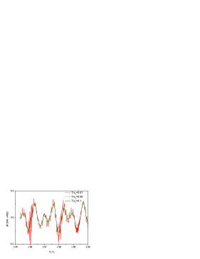
Figure 2: Oscillating magnetization for intermediate fields and three temperatures. Magic resonances are observed in many Fourier harmonics at low temperatures.

If the conventional dHvA frequency is high, $F_{0}\gg B$, three novel dHvA/SdH frequencies, $F,F^{\pm}$ of the wire can be estimated as $F=B^{2}/\delta B\simeq\mu B^{2}|df/dB|/(\hbar f^{2})$ with $f=2\omega,\omega^{\pm}$,

$$F=F_{0}/(1+\gamma)^{3/2},$$ (19)

and

$$F^{\pm}=2F_{0}/|1+\gamma\pm(1+\gamma)^{1/2}|,$$ (20)

where $F_{0}=S_{F}\hbar c/(2\pi e)$, $\gamma=4\omega_{s}^{2}/\omega_{c}^{2}=4\pi^{2}S_{F}\hbar^{2}c^{2}/(e^{2}SB^{2})$, $S=\pi R^{2}$ is the cross-section area of the wire, and $S_{F}=\pi(m^{*})^{2}v_{F}^{2}/\hbar^{2}$ is the Fermi-surface cross-section area. They are related as $F=F^{+}F^{-}|F^{+}-F^{-}|/(F^{+}+F^{-})^{2}$.

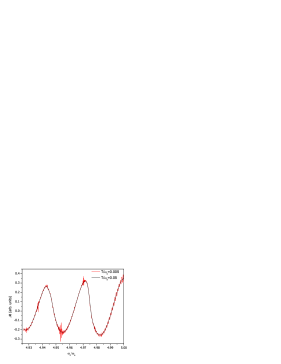
Figure 3: Oscillating magnetization for high fields and two temperatures.

Remarkably, both temperature and scattering damping factors in Eqs.(5,10) depend on $\omega$ and $\omega^{\pm}$ rather than on the cyclotron frequency $\omega_{c}$. Hence there are no constraint on the value of the magnetic field imposed by those factors as soon as $\omega_{s}$ is large enough, $\omega_{s}>T,1/\tau$. In low fields, where $\gamma\gg 1$, all frequencies are much lower than $F_{0}$, $F\approx F_{0}/\gamma^{3/2}$ and $F^{\pm}\approx 2F_{0}/\gamma$. In high fields, where $\gamma\ll 1$, two of them are about the same as $F_{0}$, $F\approx F^{+}\approx F_{0}$, while the third one appears to be much higher, $F^{-}\approx 4F_{0}/\gamma\gg F_{0}$. With respect to the Pauli paramagnetism and Landau diamagnetism in the bulk metal, amplitudes of quantum corrections in the magnetization and in the magnetic susceptibility, $\chi$, per unit volume are about $(\hbar\omega_{s}/\mu)^{1/2}$ and $[\mu/(\hbar\omega_{s})]^{1/2}$, respectively, (to get these estimates we divide $\cal{M}$ by $\pi R^{2}$). The relative amplitude of quantum corrections in the conductance is $(\hbar\omega_{s}/\mu)^{5/2}$, and about $(\hbar\omega_{s}/\mu)^{3/2}$ and $(\hbar\omega_{s}/\mu)^{1/2}$ in its first and second field derivatives, respectively. If we take $\omega_{s}$ about the same as $\omega_{c}$, the quantum corrections are much smaller than in the bulk metal, where they have the relative order of magnitude as $[\mu/(\hbar\omega_{c})]^{1/2}$ in $\cal{M}$, $[\mu/(\hbar\omega_{c})]^{3/2}$ in $\chi$ and $(\hbar\omega_{c}/\mu)^{1/2}$ in $\sigma$ shon . However, there are some ”magic” magnetic fields where the quantum corrections ”explode”. These are fields where the condition $2\omega/(\omega^{\pm})=(q+2)/r$ is satisfied, so $"\cot"$ in Eqs.(5,10) becomes infinite if $q$ is an integer. In particular, first harmonics with $r=1$ become infinite if

$${\omega_{c}\over{\omega_{s}}}={q\over{\sqrt{q+1}}}={1\over{\sqrt{2}}},{2\over{\sqrt{3}}},{3\over{\sqrt{4}}},....$$ (21)

These magic resonances are clearly seen in Figs.1,2 at low temperatures, where we present numerical data for the oscillating part of the magnetization ($\mu/\omega_{s}$ is $1000$ and we choose $\cos[\pi r\mu_{B}B/(\hbar x)]=1$). At high fields, $\omega_{c}\gg\omega_{s}$, the conventional dHvA pattern dominates, but the magic resonances are still there, Fig.3.

Let us elaborate more about the physical origin of the magic resonances. It is well known that the Landau levels are $SeB/(2\pi c\hbar)$-fold degenerate in the bulk metal of the cross-section area $S$. The boundary conditions in the nanowire (approximated here by the confinement potential) remove the degeneracy, Eq.(1). Therefore the density of states at every level is reduced by a factor $\omega_{s}^{2}/(\pi^{2}\mu\omega_{c})$, which explains the reduction of quantum amplitudes compared with the bulk metal. However, the magic resonance conditions partially restore the degeneracy of the spectrum, Eq.(1). For example, if $\omega_{c}=\omega_{s}/\sqrt{2}$, one obtains $2\omega=3\omega_{s}/\sqrt{2}$ and $\omega^{-}=\omega_{s}/\sqrt{2}$, so that $E_{\alpha}=\hbar^{2}k^{2}/(2m^{*})+\hbar\omega_{s}(6n+3|m|-m+3)/(2\sqrt{2})+s\mu_{B}B$, which is the same for all combinations of $n$ and $m$ with a fixed value of $6n+3|m|-m$. Hence, compared with the amplitudes estimated above, the magic amplitudes are enhanced. The ”anharmonic” corrections to the linearised energy spectrum in Eq.(1)imposed by the boundary conditions restrict their enhancement.

It might be difficult to observe the novel oscillations in the magnetization of a single nanowire because its small volume, but they could be measured on bundles of nanowires. As far as SdH oscillations in nanowires hub ; gro is concerned, their quantitative comparison with the present theory needs measurements in a wider field-range allowing for the reliable Fourier analysis. Using the typical radius of $Bi$-nanowires $R=100$ nm sinmol ; hub ; gro and the Fermi surface cross-section area $S_{F}=10^{13}cm^{-2}$ bhar yields an estimate of $\hbar\omega_{s}/k_{B}\approx 50K$ with the carrier mass $m^{*}=0.1m_{e}$. Then the lowest temperature presented in Figs. 1, 2 is about $0.5$ K with these parameters.

In conclusion, we have presented the theory of magnetic quantum oscillations in clean metallic nanowires with simple Fermi-surfaces. We have found novel oscillations caused by the interplay between size and field energy-level quantizations with three characteristic frequencies, calculated their amplitudes and identified magic resonances, where the quantum corrections are strongly enhanced. Our findings suggest that one can measure both reciprocal and real space geometries of nanowires in a single measurement.

References

(1)
D. Schoenberg, Magnetic Oscillations in Metals
(Cambridge University Press, Cambridge 1984).
(2)
J. Singleton, Rep. Prog. Phys. 63, 1111 (2000).
(3)
M. V. Kartsovnik, Chem. Rev. 104, 5737 (2004).
(4) for recent developments see Molecular nanowires and
Other Quantum Objects edited by A.S. Alexandrov, J. Demsar and I.K. Yanson
(Kluwer Academic Publishers, Dordrecht/Boston/London, 2004).
(5)
J. Heremans, C.M. Thrush, Y-M. Lin, S. Cronin, Z. Zhang,
M.S. Dresselhaus, and J.F. Mansfield, Phys. Rev.
B61, 2921 (2000) and references therein.
(7)
A. Bochtold, C. Strunk, J-P. Salvetat, J-M. Bonard, L. Forro,
T. Nussbaumer, and C. Schönenberger, Nature 397, 673 (1999).
(8)
A. Fujiwara, K. Tomiyama, H. Suematsu, M. Yumura and
K. Uchida, Phys. Rev. B 60, 13492 (1999).
(9)
S. Roche, G. Dresselhaus, M.S. Dresselhaus, and
R. Saito, Phys. Rev. B 62, 16092 (2000)
(10)
T.E. Huber, A. Nikolaeva, D. Gitsu, L. Konopko,
C.A. Foss Jr., and M.J. Graf, Applied Phys. Lett. 84, 1326 (2004).
(11)
A.D. Grosav and E. Condrea, J. Phys. Cond. Matter 16, 6507 (2004).
(12)
S. Tomonaga, Prog. Theor. Phys. (Kyoto) 5, 544 (1950).
(13)
A.S. Alexandrov and A.M. Bratkovsky, Phys. Rev. Lett. 76, 1308 (1996).
(14)
N. Harrison, J. Caulfield, J. Singleton, P.H.P. Reinders,
F. Herlach, W. Hayes, M. Kurmoo, and P.J. Day,
J. Phys. Condens. Matter 8, 5415 (1996).
(15)
R.A. Shepherd, M. Elliott, W.G. Herrended-Harker,
M. Zervos, P.R. Morris, M. Beck and M. Ilegems,
Phys. Rev. B 60, R11277 (1999).
(16)
Y. Yoshida, A. Mukai, K. Miyake, N. Watanabe, R. Settai,
Y. Onuki, T.D. Matsuda, Y. Aoki, H. Sato, Y. Miyamoto,
and N. Wada, Physica B281-282, 959 (2000).
(17)
A.S. Alexandrov and A.M. Bratkovsky, Phys. Let. A53, 234 (1997).
(18)
A.A. Abrikosov, L.P. Gor’kov, and I.E. Dzyyaloshinski,
Methods of Quantum Field Theory in Statistical Physics
(Prentice Hall, Englewood Cliffs, NJ, 1964).
(20)
One can also obtain this expression using the familiar Kubo
formula , where
is the z-component velocity operator and is
taken over the single-particle quantum states (see in R.
Kubo, H. Hasegava, and N. Hashitsume, J. Phys. Soc. Japan 14, 56 (1959)).