Reconstruction of Plane Circular Currents from Their Orthogonal Magnetic Field

Abstract

The solution is presented to the problem what distribution of electric current in thin circular film provides a given distribution of normal (perpendicular to film) component of the current-induced magnetic field at film’s surface.

I Introduction

Plane electric current distributions and magnetic fields produced by them are of great interest in a number of applications, for instance, when investigating magnetic flux pinning and critical states in thin superconductor films. At given current, one can calculate its field anywhere by direct integration. But in practice the inverse problem arises: how one could extract the current from measuring orthogonal (normal to plane) component of its field in some film’s neighborhood, e.g. at its surface? Although this is standard problem of the classical theory of potential, I did not find its solution in textbooks. Therefore I ventured to derive it independently, for special case of axial symmetry.

II The problem

Let a film with radius $\,R\,$ and small thickness $\,D<<R\,$ ($D/R\rightarrow 0$) lies in the $XY$-plane ($\,\rho\equiv\sqrt{x^{2}+y^{2}}<R\,$, $\,|z|<D/2\,$) and carries a circular current whose density integrated over the thickness is $\,J(\rho)\,$. We assume that in fact we know not $\,J(\rho)\,$ itself but normal component of its magnetic field close to the film’s surface, $\,H_{z}(\rho,z=\pm D/2\rightarrow 0)\,$. In case of superconductor film, this quantity represents density of vortices which pierce the film. From known $\,H_{z}(\rho,0)\,$ we want to obtain tangential radial component of same field, $\,H_{\rho}(\rho,z=D/2\rightarrow+0)=$ $-H_{\rho}(\rho,z=-D/2\rightarrow-0)\,$. If the latter is known, then the integral surface current density $\,J(\rho)=$ $\int j_{\phi}(\rho,z)dz\,$ (with $\,j_{\phi}\,$ being azimuth current density) can be found with the help of relation

$$\frac{4\pi}{c}J(\rho)=\pm\,2H_{\rho}(\rho,\pm D/2)-\frac{\partial}{\partial\rho}\int_{-D/2}^{D/2}H_{z}(\rho,z)dz\approx$$

$$\approx\,\pm\,2H_{\rho}(\rho,\pm 0)\,\,\,,$$ (1)

which follows from the Maxwell equation  curl$\,\bm{H}=4\pi\bm{j}/c\,\,$ (written in the CGSE units).

Outside the film, the field has potential character, $\,\bm{H}=-\nabla U\,$, with a potential $\,U\,$ satisfying the Laplace equation $\,\triangle U=0\,$. With reference to circular geometry, it is natural to consider the potential $\,U\,$ using the spheroidal coordinates. Their definition and examples of there application can be found e.g. in ll . We use slightly modified version of spheroidal coordinates, in the form

$$\begin{array}[]{c}\rho^{2}=R^{2}(1+u^{2})(1-v^{2})\,\,,\,\,\,z^{2}=R^{2}u^{2}v^{2}\\ \,\,\,(\,0<u^{2}<\infty\,\,,\,\,\,0<v^{2}<1\,)\,\,,\end{array}$$ (2)

at that the horizontal angle stays the third coordinate: $\,x=\rho\cos\,\phi\,$, $\,y=\rho\sin\,\phi\,$. To write the Laplace operator, $\,\triangle\,$, in these coordinates, it is convenient to introduce two operators

$$\Lambda_{-}(u)\equiv\frac{\partial}{\partial u}(1+u^{2})\frac{\partial}{\partial u}\,\,,\,\,\,\Lambda_{+}(v)\equiv\frac{\partial}{\partial v}(1-v^{2})\frac{\partial}{\partial v}\,$$ (3)

Then $\,\triangle\,$ looks as

$$\triangle=-\frac{1}{R^{2}\,(u^{2}+v^{2})}\,\left[\Lambda_{-}(u)+\Lambda_{+}(v)\right]+\,\frac{1}{\rho^{2}}\,\frac{\partial^{2}}{\partial\phi^{2}}\,\,,$$ (4)

The film occupies the region $\,\rho<R$, $z=0\,$, which corresponds to $\,u=0\,$, while the rest of the plane $\,z=0\,$ to $\,v=0\,$. Of course, the potential must be anti-symmetric with respect to this plane, therefore,

$$U(\rho>R,z=0)=U(u,v=0)=0$$ (5)

At film’s surface the potential has discontinuity, but its normal derivative is continuous. By the terms of our task,

$$\left[-\frac{\partial}{\partial z}\,U(\rho<R,z)\right]_{z=0}=\left[-\frac{1}{Rv}\,\frac{\partial}{\partial u}\,U(u,v)\right]_{u=0}=$$

$$=H_{z0}(\rho)=H_{z0}\left(R\sqrt{1-v^{2}}\right)\,\,,$$ (6)

where $\,H_{z0}(\rho)=H_{z}(\rho<R,0)\,$ is a given function. Formally, the problem $\,\triangle U=0\,$ with boundary conditions (5) and (6) is equivalent to the problem about electric potential of a charge distributed, with density $\,H_{z0}\delta(z)/2\pi\,$, in the circular hole $\,\rho<R\,$ cut out of ideally conducting plane $\,z=0$.

If the axial symmetry is assumed, then the Laplace equation reduces to

$$(\Lambda_{-}+\Lambda_{+})\,U=\,0\,\,$$ (7)

III Magnetic potential

The operator $\,\Lambda_{+}\,$ in (7) is nothing but generating operator for the complete set of orthogonal (at interval $\,-1<v<1\,$) Legendre polynomials $\,P_{n}(v)\,$ (see e.g. nu ):

$$\Lambda_{+}(v)P_{n}(v)=-\lambda_{n}P_{n}(v)\,\,,\,\,\,\lambda_{n}=n(n+1)\,\,,$$ (8)

Therefore, particular solutions to Eq.7 have the form $\,P_{n}(v)Q_{n}(u)\,$, where functions $\,Q_{n}(u)\,$ satisfy the equation $\,\Lambda_{-}(u)Q_{n}(u)=\lambda_{n}Q_{n}(u)\,$. It is easy to see that $\,\Lambda_{-}(iv)=$ $-\Lambda_{+}(v)\,$. Consequently, $\,Q_{n}(u)\propto\widetilde{P}_{n}(iu)\,$, with $\,\widetilde{P}_{n}(u)\,$ also being solutions of Eq.8: $\,\Lambda_{+}(u)\widetilde{P}_{n}(u)=-\lambda_{n}\widetilde{P}_{n}(u)\,$. That must be chosen be the second kind (non-polynomial) eigenfunctions which have zero asymptotic at infinity, because $\,U(u,v)\,$ should tend to zero at $\,z\rightarrow\infty$. Hence, according to general theory of classical special functions nu , $\,Q_{n}(u)\,$ can be represented by

$$Q_{2k}=\int_{-1}^{1}\frac{uP_{2k}(s)ds}{s^{2}+u^{2}}\,\,,\,\,\,Q_{2k+1}=\int_{-1}^{1}\frac{sP_{2k+1}(s)ds}{s^{2}+u^{2}}$$ (9)

In view of the boundary condition (5), as well as (6), the odd polynomials with $\,n=2k+1\,$ ($k=0,1,..$) only contribute to complete solution of Eq.7. By this reason, we can write

$$U(u,v)=\sum_{k=0}^{\infty}\,(4k+3)\,C_{k}\,P_{2k+1}(v)\,Q_{2k+1}(u)\,\,,$$ (10)

with coefficients $\,C_{k}\,$ to be determined from condition (6). Notice nu that $\,P_{2k+1}(v)\,$ form complete orthogonal set in the half-interval $\,0<v<1\,$. Under standard classical definition of Legendre polynomials,

$$\begin{array}[]{c}\int_{0}^{1}P_{2k+1}(s)P_{2m+1}(s)\,ds=\delta_{km}/(4k+3)\,\,,\end{array}$$ (11)

that is $\,4k+3\,$ in (10) serves as normalizing multiplier.

The result of subsequent proper calculations (detailed in Appendix in Sec.1) reads

$$C_{k}=(-1)^{k}S_{k}\int_{0}^{R}P_{2k+1}\left(\sqrt{1-\frac{r^{2}}{R^{2}}}\right)H_{z0}(r)\frac{r\,dr}{\pi R}$$ (12)

Here the quantities

$$\begin{array}[]{c}S_{k}\,\equiv\,B(1/2,k+1)/2\,=\,2^{k}k!/(2k+1)!!\end{array}$$ (13)

are introduced. At upper side of film’s surface, formulas (10) and (12), as combined with (9) and (2), yield (see Appendix 2)

$$U(\rho,z=+0)=\int_{0}^{R}G_{R}(\rho,r)\,H_{z0}(r)\,r\,dr\,\,,$$ (14)

where the Green function $\,G_{R}(\rho,r)\,$ is presented by

$$G_{R}(\rho,r)\,\equiv\,\frac{2}{\pi R}\,\sum_{k=0}^{\infty}\,(4k+3)\,S_{k}^{2}\,P_{2k+1}\left(\sqrt{1-\frac{\rho^{2}}{R^{2}}}\right)P_{2k+1}\left(\sqrt{1-\frac{r^{2}}{R^{2}}}\right)\,=$$ (15)

$$=\,\frac{2}{\pi\max(\rho,r)}\left[\,K\left(\frac{\min(\rho,r)}{\max(\rho,r)}\right)-F\left(\arcsin\frac{\max(\rho,r)}{R}\,,\,\,\frac{\min(\rho,r)}{\max(\rho,r)}\,\right)\,\right]\,=$$ (16)

$$=\,\frac{2}{\pi\,(\rho+r)}\left[\,K\left(\frac{2\sqrt{\rho r}}{\rho+r}\right)-2F\left(\frac{1}{2}\arcsin\frac{\rho}{R}+\frac{1}{2}\arcsin\frac{r}{R}\,,\,\,\frac{2\sqrt{\rho r}}{\rho+r}\,\right)\,\right]\,\,\,,$$ (17)

where $\,F(\phi,k)\,$ is the first-kind elliptic integral and $\,K(k)=F(\pi/2,k)\,$ the first-kind complete elliptic integral. The way of summation of the series (15) is described in Sec.3 of Appendix.

IV Current

Provided the normal field at surface of (infinitely) thin film is known, the current can be restored by means of (1) and (14):

$$\frac{2\pi}{c}J(\rho)=H_{\rho 0}(\rho)=-\frac{d}{d\rho}\int_{0}^{R}G_{R}(\rho,r)\,H_{z0}(r)\,r\,dr\,\,,$$ (18)

where $\,H_{\rho 0}(\rho)\equiv H_{\rho}(\rho,z=+0)\,$. Integration of (18) yields the mean current:

$$\frac{2\pi}{c}\,\frac{1}{R}\int_{0}^{R}J\,d\rho=\frac{1}{R}\int_{0}^{R}\left(1-\frac{2}{\pi}\arcsin\frac{r}{R}\right)\,H_{z0}(r)\,dr\,\,$$ (19)

It is easy to calculate also the magnetic moment, $\,M\,$, of the current mk :

$$\begin{array}[]{c}M=\frac{2}{\pi}\int_{0}^{R}r\,\sqrt{R^{2}-r^{2}}\,H_{z0}(r)\,dr\end{array}$$ (20)

Thus both these characteristics eliminate contributions from the film’s edge, i.e. $H_{z0}(\rho\approx R)\,$.

The expansion (16), when substituted to (18), determines “natural modes” of the surface field:

$$H_{z0}=h_{\perp k}(\rho)\equiv\frac{P_{2k+1}(\sqrt{1-(\rho/R)^{2}})}{\sqrt{1-(\rho/R)^{2}}}\,\,\Leftrightarrow\,\,$$ (21)

$$\Leftrightarrow\,H_{\rho 0}=h_{\parallel k}(\rho)\equiv\frac{2}{\pi}\,S_{k}^{2}\,\frac{\,\rho\,P^{\prime}_{2k+1}(\sqrt{1-(\rho/R)^{2}})}{\sqrt{R^{2}-\rho^{2}}}\,$$ (22)

Clearly, $\,h_{\perp k}(\rho)\,$ is $\,2k$-order polynomial, and $\,h_{\perp k}(0)=1\,$ (because $\,P_{n}(1)=1$), while $\,h_{\parallel k}(\rho)\,$ is polynomial of the same order multiplied by factor $\,\rho/\sqrt{R^{2}-\rho^{2}}\,$ and possesses square-root divergency at film’s edge. Both $\,h_{\perp k}(\rho)\,$ and $\,h_{\parallel k}(\rho)\,$ have $\,k\,$ zeros at $\,0<\rho<R\,$. In particular, $\,h_{\parallel 0}(\rho)=$ $2\rho/\pi\sqrt{R^{2}-\rho^{2}}\,$ determines the current distribution (see e.g. mk ) which creates constant unit-value field at film’s surface. Of course, one can form linear combinations of these modes without current’s divergency at the edge. For example, the two lowest modes ($\,k=0,1\,$) give

$$\begin{array}[]{c}H_{z0}=1-\frac{3}{2}\,x^{2}\,\,\Leftrightarrow\,\,H_{\rho 0}=\frac{4}{\pi}\,x\,\sqrt{1-x^{2}}\,\,\,,\end{array}$$ (23)

with $\,x\equiv\rho/R\,$.

The approach mentioned in Appendix 3 allows to divide (18) into singular and regular parts:

$$H_{\rho 0}(\rho)\,=\,H_{\rho 0}^{sing}(\rho)\,+\,H_{\rho 0}^{reg}(\rho)\,\,,$$ (24)

$$H_{\rho 0}^{sing}(\rho)=\frac{2\,\rho}{\pi\sqrt{R^{2}-\rho^{2}}}\int_{0}^{R}\frac{H_{z0}(r)\,r\,dr}{R\sqrt{R^{2}-r^{2}}}\,\,,$$ (25)

$$H_{\rho 0}^{reg}(\rho)=-\,\int_{0}^{R}T\left(\frac{\rho}{R},\frac{r}{R}\right)\frac{r}{R}\,\,\frac{dH_{z0}(r)}{dr}\,\,dr\,\,$$ (26)

In the latter formula,

$$T(x,y)\equiv\frac{2\,[K(k)-F(\phi,k)-E(k)+E(\phi,k)]}{\pi\min(x,y)}\,\,,$$ (27)

with $\,E(k)\,$ and $\,E(\phi,k)\,$ being the second-kind elliptic integrals whose module of ellipticity $\,k\,$ and phase $\,\phi\,$ are expressed by

$$\begin{array}[]{c}k\equiv\min(x,y)/\max(x,y)\,\,,\,\,\,\phi\equiv\arcsin\max(x,y)\end{array}$$ (28)

Clearly, $\,T(x,y)\,$ has logarithmic peak at $\,x=y\,$ (see Fig.1). What is important, $\,T(1,y)=T(x,1)=0\,$, therefore $\,H_{\rho 0}^{reg}(\rho\rightarrow R)\,$ is zero (or at least finite value). In opposite, $\,H_{\rho 0}^{sing}(\rho\rightarrow R)\,$ diverges except the cases when the integral in (25) turns into zero (e.g. in the example (23)). In such case, (18) becomes integral relation (26) between current and radial derivative of normal field (in place of differential relation $\,4\pi j/c=-\partial H_{z}/\partial\rho\,$ which would work under cylindrical geometry).

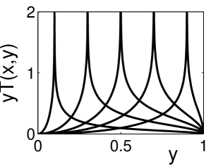
Figure 1: The kernel $\,T(x,y)\,y\,$ of the integral relating the current to the field gradient, as function of $\,y\,$ at $\,x\,=\,0.1,\,0.3,\,0.5,\,0.7$ and $0.9\,$.

V Conclusion

To resume, we found how to determine an electric current distribution in thin circular film from normal component of the current-induced field measured in the vicinity of film’s surface (very similar task about infinite strip film must be considered separately). The results can be applied, in particular, to numeric modeling of magnetic flux penetration into superconducting film.

I am grateful to Dr. Yu. Medvedev and Dr. V. Khokhlov for useful comments.

*

Appendix A

1. According to (6), (10) and (11),

$$\begin{array}[]{c}C_{k}=-[Q_{2k+1}^{\prime}(+0)]^{-1}\,\times\\ \times\,R\,\int_{0}^{1}s\,P_{\,2k+1}(s)\,H_{z0}\left(R\sqrt{1-s^{2}}\right)ds\,,\end{array}$$ (29)

where the upper half-space $\,z>0\,$ is considered, and the prime means differentiation:

$$\begin{array}[]{c}Q_{2k+1}^{\prime}(+0)\,\equiv\,\lim_{\,u\rightarrow+0}\,\,dQ_{2k+1}(u)/du\end{array}$$ (30)

From (9) it follows that at

$$Q_{2k+1}(u)=Q_{2k+1}(0)-\int_{-1}^{1}\frac{u^{2}P_{2k+1}(s)ds}{s(u^{2}+s^{2})}$$

Here in the limit $\,u\rightarrow+0\,$ factor $\,u/(u^{2}+s^{2})\,$ works as $\,\pi\delta(s)\,$, therefore

$$Q_{2k+1}^{\prime}(+0)=-\pi\lim_{s\rightarrow 0}P_{2k+1}(s)/s=-\pi\,P_{2k+1}^{\prime}(0)$$ (31)

The right-hand sides of these equalities can be easily found from the generating function of Legendre polynomials nu ,

$$\sum_{n=0}^{\infty}t^{n}P_{n}(v)=1/\sqrt{1+t^{2}-2tv}\,\,$$ (32)

Its differentiation by $\,v\,$ at point $\,v=0\,$ and Taylor expansion over $\,t\,$ show that

$$\begin{array}[]{c}P_{2k+1}^{\prime}(0)\,=\,(-1)^{k}/S_{k}\,\,\,,\end{array}$$ (33)

with $\,S_{k}\,$ defined by (13), and $\,P_{2k+1}^{\prime}(s)\equiv$ $dP_{2k+1}(s)/ds\,$. Combining (29), (31) and (33) and performing the obvious change of variables in the integral in (29), we obtain (12).

2. According to (10) and (2), to express the potential at upper film’s side, $\,U(\rho,z\rightarrow+0)=$ $U(u\rightarrow+0,v=\sqrt{1-\rho^{2}/R^{2}})\,$, we should calculate the quantities $\,Q_{2k+1}(0)\,$ determined by (9). This can be made either with the help of the recurrent relations between Legendre polynomials nu or with the help of (32). Direct integration of (32), after dividing by $\,v\,$ and replacing $\,t\,$ by $\,it\,$, yields

$$\frac{1}{2i}\,\sum_{k=0}^{\infty}\,(it)^{2k+1}\int_{-1}^{1}\frac{P_{2k+1}(v)}{v}\,dv=\frac{\arcsin\,t}{\sqrt{1-t^{2}}}\,$$ (34)

From another hand, let us pay attention to that the coefficients (13) can be represented as

$$\begin{array}[]{c}S_{k}=\int_{0}^{\pi/2}\sin^{2k+1}\theta\,d\theta\,\,\,,\end{array}$$ (35)

therefore their generating function coincides with (34):

$$\sum_{k=0}^{\infty}\,t^{2k+1}S_{k}=\int_{0}^{\pi/2}\frac{t\sin\,\theta\,d\theta}{1-t^{2}\sin^{2}\theta}=\frac{\arcsin\,t}{\sqrt{1-t^{2}}}\,$$ (36)

Comparing (36) and (34), and taking into account (9) and (13), we conclude that

$$Q_{2k+1}(0)=\int_{-1}^{1}\frac{P_{2k+1}(s)}{s}\,ds\,=\,2(-1)^{k}S_{k}$$ (37)

3. Let us consider the series

$$\sigma(x,y)\,\equiv\,\sum_{k=0}^{\infty}\,(4k+3)\,S_{k}^{2}\,P_{2k+1}(x)P_{2k+1}(y)\,\,,$$ (38)

which turns into (15) after the evident change of variables (and adding constant multiplier). One of ways to sum it is based on the remarkable formula vi :

$$\begin{array}[]{c}\sum_{n=0}^{\infty}\,(2n+1)\,P_{n}(x)P_{n}(y)P_{n}(z)\,=\\ \\ =\,\frac{2}{\pi}\,\,\mathbf{Re}\,\,1/\sqrt{1-x^{2}-y^{2}-z^{2}+2xyz}\,\,\,,\end{array}$$ (39)

where $\,-1<x,y,z<1\,$ and the symbol $\,\mathbf{Re}\,$ means taking real part, that is the right-hand side is zero when the subradical expression is negative (in vi this formula is presented in slightly different notations).

Now, divide both sides of (LABEL:vil) by factor $\,2z\,$ and integrate over $\,z\,$ from $\,-1\,$ to $\,1\,$ (in the sense of principal value). On the right-hand side we have exactly calculable integral. On the left, apply the relation (37) (clearly, the odd terms only survive, with indices $\,n=2k+1$). The result is

$$\begin{array}[]{c}g(x,y)\,\equiv\,\sum_{n=0}^{\infty}\,(4k+3)(-1)^{k}S_{k}\,P_{2k+1}(x)P_{2k+1}(y)\,=\\ \\ =\,\,\mathbf{Re}\,\,\,\mathrm{sign}(xy)\,/\sqrt{x^{2}+y^{2}-1}\end{array}$$ (40)

Next, multiply together $\,g(x,s)\,$ and $\,g(y,s)\,$ and integrate the product over $\,0<s<1\,$. On the left we should apply the orthogonality and normalization relations (11). On the right, we arrive to a standard elliptic integral, eventually obtaining the equality

$$\sigma(x,y)\,=\,\frac{\mathrm{sign}(xy)\,[K(k)-F(\phi,k)]}{\sqrt{1-\min(x^{2},y^{2})}}\,\,,$$ (41)

where $\,K(k)\,$ and $\,F(\phi,k)\,$ are standardly designated first-kind elliptic integrals (complete and incomplete, respectively) whose module of ellipticity $\,k\,$ and phase $\,\phi\,$ are expressed by

$$\begin{array}[]{c}\phi\,\equiv\,\arcsin\sqrt{1-\min(x^{2},y^{2})}\,\,\,,\\ \\ k\,\equiv\,\sqrt{[1-\max(x^{2},y^{2})]\,/\,[1-\min(x^{2},y^{2})]}\,\,\,,\end{array}$$

and function $\,\sigma(x,y)\,$ is defined by (38). Changing here $\,x\,$ and $\,y\,$ by $\,\sqrt{1-\rho^{2}/R^{2}}\,$ and $\,\sqrt{1-r^{2}/R^{2}}\,$, respectively, and multiplying the result by $\,2/\pi R\,$, we come to the relations (15)-(16). The conversion of (16) into (17) is based on properties of elliptic integrals (see e.g. kk ; dw ).

References

(1)
L. D. Landau and E. M. Lifshitz. Electrodynamics of continuous
media. Moscow, Nauka, 1982.
(2)
A. F. Nikiforov and V. B. Uvarov. Special functions of
mathematical physics. Moscow, Nauka, 1978.
(3)
N. Ya. Vilenkin. Special functions and the theory of group
presentations. Moscow, Nauka, 1991.
(4)
P. N. Mikheenko and Yu. E. Kuzovlev, Physica C 204, 229
(1993).
(5)
G. Korn and T. Korn. Mathematical handbook. McGraw-Hill, N.-Y.,
1961.
(6)
H. Dwight. Tables of integrals. Moscow, Nauka, 1970.