Magnetic-field dependence of transport in normal and Andreev billiards:
a classical interpretation to the averaged quantum behavior

Abstract

We perform a comparative study of the quantum and classical transport probabilities of low-energy quasiparticles ballistically traversing normal and Andreev two-dimensional open cavities with a Sinai-billiard shape. We focus on the dependence of the transport on the strength of an applied magnetic field $B$. With increasing field strength the classical dynamics changes from mixed to regular phase space. Averaging out the quantum fluctuations, we find an excellent agreement between the quantum and classical transport coefficients in the complete range of field strengths. This allows an overall description of the non-monotonic behavior of the average magnetoconductance in terms of the corresponding classical trajectories, thus, establishing a basic tool useful in the design and analysis of experiments.

I Introduction

Ballistic transport of particles across billiards is a field of major importance due to its fundamental properties as well as physical applications (see for example the reviews QuaCh ; Alha ; Ri00 ; Jalab ). In such systems, a two-dimensional cavity is defined by a steplike single-particle potential where confined particles can propagate freely between bounces at the billiard walls. For open systems the possibility of particles being injected and escaping through holes in the boundary is also allowed. As an example, we consider the open geometry of the extensively studied Sinai billiard shown in Fig. 1. Experimental realizations are based on exploiting the analogy between quantum and wave mechanics in either microwave and acoustic cavities or vibrating plates QuaCh , and on structured two-dimensional electron gases in artificially tailored semiconductor heterostructures Alha ; Ri00 ; Jalab . In the latter case, the particles are also charge carriers making these nanostructures relevant to applied electronics.

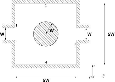
Figure 1: The open geometry of the Sinai billiard considered in this study.

Focussing the attention on the electronic analogues, more recently the possibility to couple a superconductor to a ballistic quantum dot has been considered both theoretically KosMasGol ; S-billiards and experimentally EPL02ETW , so that some part of the billiard boundary exerts the additional property of Andreev reflection And64 . During this process particles with energies much smaller than the superconducting gap $\Delta$ are coherently scattered from the superconducting interface as Fermi sea holes back to the normal conducting system (and vice versa). Classically, Andreev reflection manifests itself by retroreflection, i.e., all velocity components are inverted, compared to the specular reflection where only the boundary normal component of the velocity is inverted. Thus, Andreev reflected particles (holes) retrace their trajectories as holes (particles). If, however, a perpendicular magnetic field is applied in addition, such retracing no longer occurs due to the inversion of both the charge and the effective mass of the quasiparticle resulting in opposite bending. Typical trajectories are illustrated in Fig. 2. Here, we investigate the interplay between trajectory bending and Andreev reflection and demonstrate how such effects influence the overall (magneto)transport properties of Andreev billiards when compared to their normal counterparts.

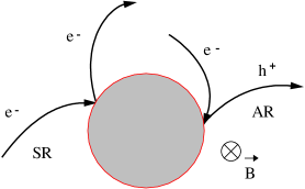
Figure 2: Typical specular (SR) and Andreev reflection (AR) at the circular central “antidot” of Fig. 1. A magnetic field is applied as indicated.

A unique feature of this class of (quantum) mechanical systems is their suitability for studying the quantum-to-classical correspondence. In particular, much effort has been devoted in revealing the quantum fingerprints of the classical dynamics which may be parametrically tuned from regular to chaotic via, e.g., changes in the billiard-shape. A range of theoretical tools has been used, spanning the usual analysis of classical trajectories and the semiclassical approximation to the models of Random Matrix Theory and fully quantum mechanical calculations. The main signatures of classical integrability (or lack of it) on the statistics of energy levels and properties of the transport coefficients for closed and open systems, respectively, have been discussed in detail in various reviews QuaCh ; Alha ; Ri00 ; Jalab . Discussions on modifications owing to the possibility of Andreev reflection appear in more recent studies KosMasGol ; MBFC96 ; S-billiards ; PRB00CBA ; PRL99SB ; EPJB01ILV ; TA01 ; PRB04CPP ; FTPR05 , mostly focusing on the features of the quantum mechanical level density.

In a similar fashion, the aim of this paper is to determine how far a purely classical analysis may provide qualitative rationalization and quantitative predictions for the average quantum mechanical transport properties of a generic billiard such as that of Fig. 1; both in the presence or absence of Andreev reflection. Indeed, by performing exact calculations for the classical and quantum dynamics of low-energy quasiparticles we find that the classical transport probabilities of electrons and holes, if appropriate, are in good quantitative agreement with the mean value (to be defined below) of the corresponding quantum mechanical scattering coefficients that determine the magnetoconductance of such systems. While most of the previous works considered the case of zero or small magnetic field (such that the classical dynamics is not altered), we particularly analyse the regime of finite magnetic field strengths and show that the classical trajectories which depend parametrically on the applied magnetic field suffice to describe the overall features of the observed non-monotonic behavior.

The article is structured as follows. In Sec. II, after a brief discussion on the details of the studied system, we present precise numerical results of the magnetic-field dependence of the transport coefficients as determined by the quantum mechanical scattering matrix. In Sec. III we first discuss the model describing the corresponding classical dynamics and provide an analysis for both the normal and the Andreev version of the Sinai billiard in Sections III.2 and III.3, respectively. A synopsis is given in Sec. IV.

II Quantum mechanical transport properties

We consider ballistic transport of charge carriers in the $2D$ Sinai-billiard shown in Fig. 1 under an externally applied magnetic field. The side length of the square cavity is taken $L=5W$ where $W$ is the width of each of the leads attached to the left and right of the cavity. The latter define source and sinks of (quasi)particles. The central scattering disk possesses the radius $R=W$, and it can be either a normal or a superconducting antidot. In the former case the antidot represents an infinitely high potential barrier while in the latter case it is considered as an extended homogeneous superconductor characterized by the property of Andreev reflection KosMasGol . Experimentally, such antidot structures have been realized in periodic arrangements, thus forming superlattices Ri00 ; EPL02ETW . The boundaries of the square cavity, numbered clockwise by the labels 1 through 4, are always normal conducting potential walls of infinite height.

In the presence of a superconductor the quantum dynamics of the system can be described by the Bogoliubov-deGennes Hamiltonian:

$$\mathcal{\hat{H}}=\left(\begin{array}[]{cc}\hat{H}_{0}&\hat{\Delta}\\ \hat{\Delta}^{*}&-\hat{H}_{0}^{*}\end{array}\right),$$ (1)

where the diagonal operators determine the motion of particles and holes, respectively, and the off-diagonal elements take care of the coupling between particle- and hole-like excitations. Later, in our classical calculations we assume perfect Andreev reflection meaning that all particles that hit the normal-superconducting (NS) interface are exactly retroreflected. In order to model this quantum mechanically we have to consider perfect coupling between the normal-conducting region and the superconductor and simulate a bulk superconductor. To this end, we take its size to be much larger than the superconducting coherence length $\xi_{S}=\hbar v_{F}/2\Delta$; $v_{F}$ is the Fermi velocity. Under these conditions, it is sufficient to consider a stepfunction-like behavior of the pair potential so that $\Delta=\Delta_{0}$ is constant inside the superconducting region and zero outside. We also assume that the temperature is sufficiently smaller than the superconducting critical temperature so that $\xi_{S}$ does not diverge.

For our numerical calculations we use a discretized version of the Bogoliubov-deGennes Hamiltonian (1) resembling the tight-binding approximation on a square lattice FTPR05 . Hence, $\hat{\mathcal{H}}$ becomes a matrix where only coupling between neighboring lattice sites is considered. The submatrix $[H_{0}]_{ij}$ has elements $\epsilon_{i}-E_{F}$ for $i=j$ and $\gamma_{ij}$ for nearest neighbors $i$ and $j$. The Fermi energy $E_{F}$ is set to a value that allows six open channels in the leads. The pairing matrix is given by $[\Delta]_{ij}=\Delta_{0}\delta_{ij}$ if lattice point $i$ is inside the superconducting region and it is zero otherwise. To reproduce the correct dispersion relation in the continuum limit the onsite energies $\epsilon_{i}$ and the hopping energies $\gamma_{ij}$ have to fulfill the relation $\epsilon_{i}=\sum_{\langle i,j\rangle}\gamma_{ij}$, where $\langle i,j\rangle$ denotes a summation over nearest neighbors $j$ of site $i$, see e.g. Ref. Fer97, .

In the presence of a magnetic field the hopping energies acquire a phase according to the Peierls substitution Fer97 , $\gamma_{ij}=-\exp[2\pi i\vec{A}\cdot(\vec{r}_{i}-\vec{r}_{j})/\Phi_{0}]$. Here, $\vec{A}$ is the vector potential, $\vec{r}_{i}-\vec{r}_{j}$ is the vector pointing from site $j$ to site $i$ and $\Phi_{0}=h/e$ is the flux quantum. In general, the pair potential $\Delta_{0}\exp{[i\chi(\vec{A})]}$ is also a complex number. However, it can be chosen real ($\chi\equiv 0$) if the vector potential $\vec{A}$ is parallel to the screening currents near the NS interface Ket99 . This is achieved by choosing the symmetric gauge $\vec{A}=[(B/2)z,0,-(B/2)x]$ that accounts for a homogeneous magnetic field of strength $B$ in $y$ direction, perpendicular to the two-dimensional system. In what follows, we define as magnetic field unit the value $B_{0}=mv_{F}/(-q_{e}W)$ for which the cyclotron radius is equal to $W$.

The transport coefficients are calculated via a recursive decimation method, as explained in Ref. Tad99, . This method enables the exact computation of the full scattering matrix $S_{n,n^{\prime}}(\varepsilon,\hat{H})$, which yields scattering properties of quasiparticles with energy $\varepsilon$, incident on a phase-coherent structure described by a Hamiltonian $\hat{H}(\vec{B})$. $\left|S_{n,n^{\prime}}(\varepsilon,\hat{H})\right|^{2}$ is the outgoing flux of quasiparticles along channel $n$, arising from a unit incident flux along channel $n^{\prime}$. The quantum numbers $n$ indicating open scattering channels are conveniently written as $n=(i,\alpha,\nu)$, where $i$ indicates the leads, $\alpha$ takes the discrete values $e$ and $h$ for particles and holes, respectively, and $\nu$ labels the quantum numbers associated with the quantization of the wavefunction in the transverse direction. As shown in Ref. Lam93, , transport properties are determined by

$$P^{\alpha,\beta}_{i,j}(\varepsilon,\hat{H})=\sum_{\nu,\nu^{\prime}}\left|S_{(i,\nu),(j,\nu^{\prime})}^{\alpha,\beta}(\varepsilon,\hat{H})\right|^{2},$$

which is referred to as either a reflectance $R$ ($i=j$) or a transmittance $T$ ($i\neq j$) from quasi-particles of type $\beta$ in lead $j$ to quasi-particles of type $\alpha$ in lead $i$. After normalization to unity with the number of open channels $N_{\rm ch}$, $\alpha\neq\beta$, $P^{\alpha,\beta}_{i,j}(E,H)$ defines the Andreev scattering probability, while for $\alpha=\beta$, it indicates a normal scattering probability. Such normalized quantities are equivalent to an angle-average and can be directly compared to the corresponding classical probabilities.

In the remaining of the article we focus on the low-energy solutions of Eq. (1) with quasiparticle energy $\varepsilon=0$, which is appropriate for the model of perfect Andreev reflection at the NS interface. In this case, particle and hole coefficients coincide. Hence, we adopt the shorthand notation $R_{e}\equiv R^{ee}/N_{\rm ch}=R^{hh}/N_{\rm ch}$, $R_{h}\equiv R^{he}/N_{\rm ch}=R^{eh}/N_{\rm ch}$ and $T_{e}\equiv T^{ee}/N_{\rm ch}=T^{hh}/N_{\rm ch}$, $T_{h}\equiv T^{he}/N_{\rm ch}=T^{eh}/N_{\rm ch}$ to indicate reflection and transmission probabilities, respectively.

Due to interference effects, quantum scattering coefficients are rapidly oscillating functions of the Fermi energy. Therefore, in order to remove the quantum fluctuations, we perform an energy average over values $k_{F}W/\pi\in[6.2,6.8]$, which corresponds to six open channels in the leads, $N_{\rm ch}={\rm Int}[k_{F}W/\pi]$, for each value of the magnetic field. The remaining parameters of our simulations are as follows. The width $W$ of the lead is $25a_{m}$. For the superconducting antidot, we define the pair potential via $\Delta=\hbar v_{F}/2\xi_{S}$ by choosing $\xi_{S}=8a_{m}$ so that the diameter $2W$ is approximately 6 times larger than the superconducting coherence length. To define the tunnel barrier in the case of the normal antidot, an onsite potential of $100\times\hbar^{2}/2ma_{m}^{2}$ is added to all lattice sites lying inside. Note that the mesh lattice constant $a_{m}$ need not be defined explicitly if all energies are measured in $\hbar^{2}/2ma_{m}^{2}$ yielding $\gamma_{ij}=1$ for every $i,j$-pair. The above definitions are consistent with the requirements set in Ref. FTPR05, about lengthscales, namely, $\xi_{S},\lambda_{F}\gg a_{m}$ and $\xi_{S}/\lambda_{F}>1$. Here, $\lambda_{F}$ is the Fermi wavelength.

Figure 3: Magnetic field dependence of the classical (solid line) and quantum (dots) transmission probability for the normal conducting Sinai billiard of Fig. 1. The magnetic field is in units of the strength $B_{0}$ for which the cyclotron radius is equal to $W$.

First we consider the Sinai billiard with a normal antidot in the center acting as a potential barrier. In this case coefficients with $\alpha\neq\beta$, i.e., involving particle-to-hole conversion (and vice-versa) are identically zero as there is no Andreev reflection at the antidot boundary. Particles (holes) can be either normally transmitted or reflected. In Fig. 3, the smoothed transmission is compared to the classical curve (Sec. III.2) revealing the same qualitative features. Even more remarkably, we see a very good quantitative agreement between both curves with deviations being within the amplitude of the small oscillations. Reflection is just symmetric to the transmission, i.e. $R_{e}=1-T_{e}$, as both the classical and the quantum calculation respect unitarity.

(a)

(b)

Figure 4: Panel (a) shows the transport coefficients of particles escaping the Andreev version of the Sinai billiard of Fig. 1 without particle-to-hole conversion. Panel (b) shows the Andreev reflection and transmission probabilities. In both panels the solid (dashed) line is the classical result of transmission (reflection) and the circles (squares) show the quantum transmission (reflection) coefficients normalized by $N_{\rm ch}$. The field strength is given in units of $B_{0}$. Inset: semilogarithmic blow up for $0.75\leq B/B_{0}\leq 1.25$.

Second we consider the case where the central antidot becomes superconducting. Andreev reflection now gives rise to non-zero $R_{h}$ and $T_{h}$ coefficients as shown in panel (b) of Fig. 4. Upon comparison of the quantum results with the classical curves, we see again that they agree very nicely. The results are summarized in Fig. 4 with vertical lines indicating two distinct values of the magnetic field, $B_{c,1}$ and $B_{c,2}$, that are related to different qualitative features in the classical dynamics. The largest differences occur for the particle-to-hole coefficients at the first critical field $B_{c,1}$. There, the classical transmission and reflection vanish abruptly, whereas the averaged quantum mechanical coefficients decay exponentially (see inset of Fig. 4). However, we leave the analysis of such effects as well as the overall non-monotonic behavior with respect to the magnetic field for the next section for a discussion under the prism of the properties of the classical trajectories.

To conclude this section, we would like to show how the conductance, as an experimentally accessible quantity, changes when the antidot is made superconducting. In Fig. 5, the magnetoconductance of a normal (dots) and for a superconducting (solid line) antidot is plotted. In the normal case the linear-response low-temperature conductance is simply proportional to the transmission $T_{e}$, according to Landauer’s formula $G_{N}=(2e^{2}/h)\;T_{e}$. Lambert et al Lam93 have worked out generalizations for systems including superconducting islands or leads. For the Andreev version of the Sinai billiard system of Fig. 1, the conductance is given by $G_{S}=(2e^{2}/h)\;(T_{e}+R_{h})$. Overall, we see that in the presence of Andreev reflection the conductance of the system is larger than in the normal conducting case for magnetic fields $B<B_{c,1}$. For larger fields the particle-to-hole coefficients vanish and the conductances for both cases almost coincide.

Figure 5: Magnetoconductance for the normal (dots) and the Andreev (solid line) Sinai-shaped billiard of Fig. 1 (in units of the number of open channels, $N_{\rm ch}$, times the conductance quantum $G_{0}\equiv 2e^{2}/h$). The field strength is in units of $B_{0}$.

III Classical dynamics

III.1 General features

In this section we study the classical dynamics of the incoming particles (we focus on electrons but the same arguments apply to incoming holes) for each of the two antidot structures described above.

The general form of the Hamiltonian describing the dynamics of charged particles inside the cavity reads

$$H=\frac{1}{2m^{*}_{\alpha}}(\vec{p}-q_{\alpha}\vec{A})^{2}.$$ (2)

The index $\alpha$ is used to describe the possibility that the propagating particles are either electrons ($e$) or holes ($h$). This generalization is necessary for a correct description of the dynamics in the setup with the superconducting antidot. The canonical momentum vector is $\vec{p}=(p_{x},p_{z})=m^{*}_{\alpha}\vec{v}+q_{\alpha}\vec{A}$ where $\vec{v}$ is the mechanical velocity, the corresponding position vector being $\vec{r}=(x,z)$. Charge conservation yields $m^{*}_{h}=-m^{*}_{e}$ for the effective masses and $q_{h}=-q_{e}$ for the electric charge. The main property which distinguishes the two cases, i.e., normal/superconducting antidot, is the interaction of the charged particle with the scattering disk. The latter is captured by the elementary processes illustrated in Fig. 2, namely, specular reflection (SR) versus the Andreev reflection (AR).

In what follows, we calculate the electronic transport properties by analyzing the ballistic propagation and escape of classical particles injected into the billiard via the opening pipe-like channels (see Fig. 1). The initial conditions for incoming electrons are determined by the phase-space density

$$\begin{split}\rho_{o}&(x,z,v_{x},v_{z})=\frac{1}{2m^{*}_{e}vW}\delta(x+\frac{L}{2})\times\\ &\left[\Theta(z+\frac{W}{2})-\Theta(z-\frac{W}{2})\right]\delta(m^{*}_{e}(v-v_{F}))\cos\theta,\\ \end{split}$$ (3)

where $\theta\in[-\frac{\pi}{2},\frac{\pi}{2}]$ is the angle of the initial electron momentum with the $x$-axis and $v_{F}=\sqrt{2E_{F}/m^{*}_{e}}$ and the coordinate origin is assumed at the center of the cavity.

The trajectories of the charged particles in the billiard consist of segments of circles with cyclotron radius $r=m^{*}_{\alpha}v/(-q_{e}B)$ (with $v=\sqrt{v_{x}^{2}+v_{z}^{2}}$). At non-vanishing external field the classical dynamics of both the normal and Andreev billiards is characterized by a mixed phase space of co-existing regular and chaotic regions. At $B=0$ the superconducting antidot leads to an integrable dynamics, (since trajectories are precisely retraced after retroreflection), while the corresponding normal device possesses a mixed phase space. It is convenient to write the dynamics (collisions with the walls and the antidot) explicitly in the form of a discrete map. As the magnitude of the velocity remains constant in time, a simple parameterization of the dynamics is given by determining the position $(x_{n},z_{n})$ of the $n$-th collision with the boundary and the angle $\theta_{n}$ of the velocity vector with respect to the normal of the boundary at the collision point taken after the collision. Here, the term boundary refers to the walls 1 throughout 4 and the circumference of the antidot (see Fig. 1).

There are three families of periodic orbits each forming a continuous set that occur in the classical dynamics and phase space of the closed system GasDor ; Kov ; SilAgu , i.e. without leads, leaving their fingerprints in the open system with the attached leads. We will briefly discuss these periodic orbits in the following. At zero field there are orbits bouncing between two opposite walls with velocities parallel to the normal of the corresponding walls. At finite but weak $B$-field strength the periodic orbits form a rosette and incorporate collisions with the antidot and the walls. These periodic orbits are typical, i.e. dominant up to a critical field value $B_{c,2}$. For magnetic fields above $B_{c,2}$ the cyclotron radius is so small that no collisions with the antidot can occur and skipping orbits, describing the hopping of the electrons along the billiard walls, become dominant. All periodic orbits possess an eigenvalue one of their stability matrix FliSchSpo and all periodic orbits possess unstable directions. We remark that the above-discussed periodic orbits of the closed billiard are not trajectories emerging from and ending in the leads of the open billiard. However, trajectories of particles coupled to the leads (i.e., injected and transmitted/reflected) can come close to the periodic orbits of the open billiard thereby tracing their properties. This way the presence of the periodic orbits reflects itself in the transport properties.

III.2 Sinai billiard with normal antidot

First we consider the transport of electrons through the Sinai billiard (Fig. 1) with a normal antidot. The relevant quantities determining the current flow through the device are the transmission $T_{e}$ and reflection $R_{e}$ coefficients for electrons defined as the percentage of the initial electrons leaving the device from the right and left lead, respectively. Additional quantities that are helpful for an understanding and analysis of the system dynamics are the mean number of collisions per incoming electron with the walls (1-4), $\langle n\rangle_{w}$, and with the antidot, $\langle n\rangle_{a}$. We calculate these quantities by numerical simulation for different values of the external magnetic field $B$. It is convenient to use a dimensionless form of the classical equations of motion by employing the scaling $x=\xi_{x}W$ and $z=\xi_{z}W$ for the spatial coordinates and $t=\tau/\omega$ (with $\omega=B_{0}/m^{*}_{e}$) for the time coordinate. The above quantities are calculated for 100 values of the magnetic field strength varying from 0.02 to 2 using an ensemble of $10^{6}$ different initial conditions distributed according to Eq. (LABEL:eq:density) for each $B$-field value. The magnetic field dependence of the coefficients $T_{e}$ and $R_{e}$ is shown in Fig. 6a. The obtained curves are quite irregular, possibly indicating the presence of fractal fluctuations in the magnetoconductance of the system Ketz .

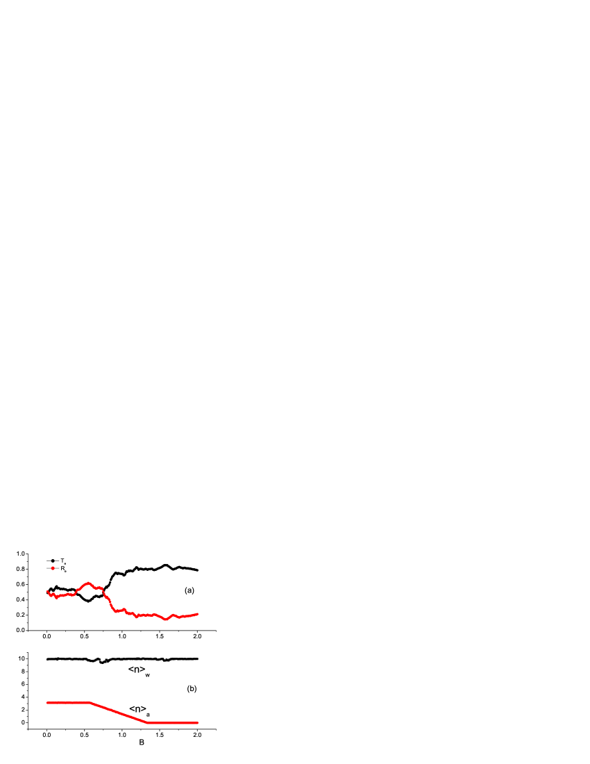
Figure 6: (a) Classical electron transmission, $T_{e}$, and reflection, $R_{e}$, coefficients for the normal antidot device of Fig. 1 as a function of the applied magnetic field $B$. (b) The mean number of collisions with the boundary of the square cavity (walls 1-4), $\langle n\rangle_{w}$, and with the circumference of the antidot, $\langle n\rangle_{a}$, as a function of $B$. The field strength is given in units of $B_{0}$.

In Fig. 6b, we present the parametric dependence of the mean quantities $\langle n\rangle_{w}$ and $\langle n\rangle_{a}$. Interestingly, the mean number of collisions with the walls remains constant $\langle n\rangle_{w}\approx 10$ for almost all values of the field strength. This means naturally that also the accumulated number of collisions of all injected trajectories with the walls is independent of the field strength for the whole regime considered. This number is obtained by integrating the occupancy of the trajectories in phase space, i.e., their measure, over all possible velocities and the boundary of the cavity (defined by the walls 1-4 including the leads). Its invariance with respect to the field strength is of combined geometrical and dynamical origin and can be understood as follows. The escape probability is well approximated by $P=\mu_{\rm esc}/\mu_{T,b}$ where $\mu_{\rm esc}$ is the measure of phase space points on the left and right leads visited by the escaping electrons, while $\mu_{T,b}$ is the total measure involved in the dynamics of the system along the boundary defined by the walls 1-4 (including the leads). The corresponding integrals can be estimated as $\mu_{\rm esc}=2c_{l}W$ and $\mu_{T,b}=4c_{b}L$. Here, $c_{l}$ is the mean phase space density on the leads and $c_{b}$ is the mean phase space density on the entire boundary, both integrated over the momenta. Due to the symmetric setup of the leads relative to both the $x$ and $z$ axis, we have $c_{l}=c_{b}=c$. Thus, $P=1/10$ and the mean number of collisions with the wall is $\langle n\rangle_{w}=1/P=10$.

The behavior of $\langle n\rangle_{a}$ is more complicated because the dynamical occupation of the antidot’s circumference strongly depends on the value of the external field. One can clearly distinguish three regimes: (i) the low field region ranging from $B\approx 0$ to $B=B_{c,1}\approx 0.55$, (ii) the intermediate field region with $B_{c,1}<B<B_{c,2}(\approx 1.33)$, and (iii) the high field region with $B>B_{c,2}$. All three regions are characterized by different properties of the corresponding phase space. These are revealed by the study of the phase space structure using Poincaré surfaces of section (PSOS) for different values of the applied field $B$. We employ $(x,v_{x})$ sections defined by the condition $z=0$. It turns out that all calculated surfaces of section reveal a mixed phase space. To further quantify our analysis we calculate the relative weight $w_{c}$ of those trajectories on the PSOS that exhibit collisions with the antidot. Since collisions with the antidot are the only possibility to obtain dynamics that is sensitive with respect to the initial conditions, $w_{c}$ is also a measure for chaoticity in phase space comm1 . We partition the energetically allowed phase space on the $(x,v_{x})$ plane into $N=10^{4}$ cells of equal size and define on each cell ${\cal{C}}_{i}$ the characteristic function $h_{{\cal{C}}_{i}}(x,v_{x})$ as:

$$h_{{\cal{C}}_{i}}=\left\{\begin{array}[]{l}1~{}~{}~{}\textup{if an orbit exists with}~{}(x,v_{x})~{}\in{\cal{C}}_{i}\\ ~{}~{}~{}~{}~{}\textup{that hits the antidot,}\\ 0~{}~{}~{}\textup{if}~{}(x,v_{x})~{}\not\in{\cal{C}}_{i}~{}\textup{holds for {\it all}}\\ ~{}~{}~{}~{}~{}\textup{trajectories hitting the antidot.}\\ \end{array}\right.$$ (4)

We subsequently approximate $w_{c}\approx(1/N)\sum_{i=1}^{N}h_{{\cal{C}}_{i}}$.

The function $w_{c}(B)$ is shown in Fig. 7. The initial plateau at $w_{c}\approx 0.5$ shows clearly that the system is to a large portion chaotic for low magnetic fields. This explains the fact that in this range of fields the mean number of collisions with the antidot $\langle n\rangle_{a}$ is almost constant. The degree of chaos in the phase space of the system is large enough thereby ensuring that, with the exception of trajectories of negligible measure, each trajectory hits the circumference of the antidot. Hence, as evaluated in a similar fashion to $\mu_{T,b}$, the total measure of phase space points $\mu_{C,a}$ involving the circumference is equal to $2\pi cW$. Following the arguments given above for $\langle n\rangle_{w}$, we estimate $\langle n\rangle_{a}$ as $\langle n\rangle_{a}/\langle n\rangle_{w}=\mu_{C,a}/\mu_{T,b}=2\pi cW/(4cL)$, yielding $\langle n\rangle_{a}\approx\pi$, which is in very good agreement with Fig. 6b. In the intermediate field region the weight of the chaotic trajectories decreases almost linearly and becomes vanishingly small in the high field region. The linear decrease of $w_{c}$ leads to a linear decrease of $\langle n\rangle_{a}$ for this range of magnetic fields. Above $B_{c,2}$ the cyclotron radius of the electron trajectories is so small ($r<L/4-W/2$) that no collision with the antidot is possible, i.e., $\langle n\rangle_{a}=0$.

Figure 7: Relative weight of the chaotic part $w_{c}$ of the phase space as a function of the applied field $B$ (in units of $B_{0}$) for the normal conducting Sinai-shaped billiard of Fig. 1.

We can now understand the non-monotonic behavior of the functions $T_{e}(B)$, $R_{e}(B)$ by considering the representative trajectory dynamics for various $B$-values. According to Fig. 6a the low field region possesses two subregions: (i) $0<B<0.4$ and (ii) $0.4<B<0.55$. Similarly the intermediate field region can be divided to: (i) $0.55<B<0.75$ and (ii) $0.75<B<1.33$. Note that the points defining the magnetic field windows, $B\approx 0.4,0.55,0.75$ and $1.33$, also mark qualitative changes in the functions $\langle n\rangle_{a}(B)$ and $w_{c}(B)$.

At very low fields, $B\rightarrow 0$, we observe that $R_{e}$ is slightly larger than $T_{e}$. This owes to many trajectories exhibiting only one collision with the antidot and reflected directly back to the lead from where they came. The typical configuration consists of an incoming electron moving almost as a free particle, hitting the antidot once, and escaping from the billiard to the left lead (electron reflection). Otherwise, in the low field region (i) the main process is the transmission of electrons. As the magnetic field increases, the reflection angle at the circumference of the antidot increases too and the incoming electron, after hitting the antidot, suffers two or more collisions with some of the walls 1,2,3 or 4 before escaping to the right lead (electron transmission). This mechanism, along with a significant amount of electrons that are initially emitted with a larger angle ($|\theta|>\tan^{-1}(2/5)$), hitting directly the upper or lower wall of the cavity (or even its right wall) suffering specular reflection and exiting to the right lead of the device, establishes electron-transmission as the main process in the low field region. However, it is evident from Fig. 6a that the difference between $T_{e}$ and $R_{e}$ is quite small. There are complex trajectories with more than 10 collisions with the walls and 5-8 collisions with the antidot possessing a finite measure in phase space. These give a non-vanishing contribution to $R_{e}$ thereby maintaining its mean value around $0.45$. In fact $T_{e}$ and $R_{e}$ fluctuate insignificantly around their mean values ($0.55$ for $T_{e}$ and $0.45$ for $R_{e}$). As the fields increases above $B=0.4$, trajectories with a larger number of collisions with the walls may become statistically more important but as long as $B<0.55$ the trajectories with several collisions with the antidot have still a significant measure (see Figs. 7 and 6b, respectively). Overall, for $0.4<B<0.55$, the main process is the reflection of electrons yielding a large difference between $T_{e}$ and $R_{e}$. Typical trajectories have one or two collisions with the walls and a single collision with the antidot. The incoming electron hits the antidot once, is specularly reflected and escapes from the billiard to the left lead, after suffering one more collision with the wall 4.

At intermediate fields, we observe an almost monotonic decrease of $R_{e}$ and an increase of $T_{e}$ owing to the combined decrease of $\langle n\rangle_{a}(B)$ and $w_{c}(B)$. The small plateau feature in Fig. 7 around $w_{c}=0.6$ is also reflected in the change of slope in the transport probabilities within subregion (i). At its upper limit, $B=0.75$, the two coefficients become equal, $T_{e}=R_{e}$. Most trajectories have $5-8$ collisions with the walls and $1-4$ collisions with the antidot. In window (ii) of the intermediate-field region with $B>0.75$, the process of transmission is much stronger than the process of reflection. Most trajectories have a few ($\approx 5$) collisions with the walls and no collision with the antidot. A typical trajectory of the incoming electron, due to the small cyclotron radius, suffers one collision with wall 1, three collisions with wall 4, one collision with wall 3 (5 collisions with the walls in total) and then escapes from the cavity through the right lead (electron-transmission). There is also the case in which the incoming electron misses the right lead of the device, and after suffering many collisions with the walls finally escapes to the left lead, contributing to the process of reflection. The same scenario is valid also for the high field region.

III.3 Sinai billiard with superconducting antidot

Compared to the dynamics of the cavity with the normal antidot, the Andreev Sinai billiard with the central superconducting disc exhibits basic differences due to the occurrence of trajectories which suffer Andreev reflection, instead of specular reflection, at the circumference of the antidot. First, the complete description of the transport properties of the system requires the introduction of two additional coefficients describing electrons that escape as holes either to the left or the right lead; $R_{h}$ (reflection) and $T_{h}$ (transmission), respectively.

In Figs. 8a and 8b, all probabilities are plotted as a function of the applied field $B$. In Fig. 8c, we present the quantities $\langle n\rangle_{w}(B)$ and $\langle n\rangle_{a}(B)$ following the definition of Sec. III.2. $T_{\alpha}$ and $R_{\alpha}$ (with $\alpha=e,h$) exhibit irregular fluctuations as a function of $B$, similar to those obtained for the normal billiard. The function $\langle n\rangle_{w}$ is almost identical to the corresponding function obtained for the normal case. Qualitatively, the mean number $\langle n\rangle_{a}$ of collisions with the superconducting antidot is also similar to that in Fig. 6b. However, while $B_{c,2}$ is remaining the same, the value of the critical field $B_{c,1}$ is shifted to the larger value $B_{c,1}\approx 0.95$. The former should be expected since it does not involve any collisions with the superconducting disc.

The difference in $B_{c,1}$ is explained by calculating the relative weight of the chaotic trajectories as in Sec. III.2. The result is shown in Fig. 9. For magnetic fields up to $B\approx 0.95$ a large part of the phase space of the system is chaotic ensuring the equal mean phase space density on the boundary of the square cavity and the circumference of the antidot. For $B>0.95$ an almost linear decrease of $w_{c}$ leads to a corresponding linear decrease of $\langle n\rangle_{a}$. At $B\approx 1.33$ the chaotic part of the phase space vanishes due to the fact that no collisions with the defocusing perimeter of the antidot are possible. An additional peculiarity of the superconducting device appears for the intermediate field region, $0.95<B<1.33$: All possible trajectories possess an even number of collisions with the antidot, yielding a vanishing transmission and reflection of holes, $T_{h}=R_{h}=0$. This interesting feature is related to the generic properties of Andreev reflection and is analyzed in Appendix A.

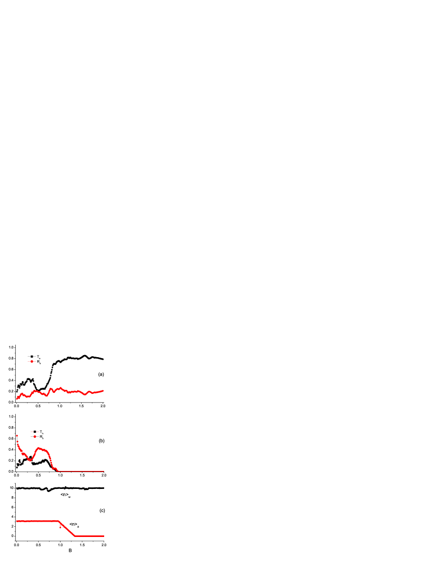
Figure 8: Classical results for the billiard of Fig. 1 with a superconducting disc in the center, as a function of the applied magnetic field $B$ (in units of $B_{0}$). (a) Classical electron transmission, $T_{e}$, and reflection ($R_{e}$) coefficients. (b) Classical electron-to-hole (Andreev) transmission, $T_{h}$, and reflection, $R_{h}$, probabilities. (c) mean number of collisions, $\langle n\rangle_{w}$, with the boundary of the square cavity (walls 1-4) and with the circumference of the antidot, $\langle n\rangle_{a}$.

Let us now consider the transport coefficients in more detail. Following the qualitative features in Figs. 8a and 8b, we divide the low field region into four windows: (i) $0<B<0.3$, (ii) $0.3<B<0.5$, (iii) $0.5<B<0.7$ and (iv) $0.7<B<0.95$. Note that different regimes roughly coincide with different qualitative features of the functions $\langle n\rangle_{a}(B)$ and $w_{c}(B)$, as indicated previously.

Figure 9: Relative weight of the chaotic part of the phase space $w_{c}$ as a function of the applied field $B$ (in units of $B_{0}$) for the Andreev version of the billiard in Fig. 1.

In region (i), due to the large cyclotron radius (almost vanishing curvature) most trajectories have a single collision with the antidot. In fact, at very small fields, $B\sim 0.01$, there is practically no collision with the walls. The typical process consists of an incoming electron moving almost on a straight line hitting the antidot once, being converted into a hole which nearly retraces the electron path moving towards the left lead and finally leaving the device. Therefore, $R_{h}$ in this region is larger than $T_{h}$, $T_{e}$ and $R_{e}$. There is however a significant amount of electrons emitted initially with a large enough angle, $|\theta|>\tan^{-1}(2/5)$, which hit directly the upper or lower wall of the device suffering normal reflection and then exiting to the right lead. This process gives a finite electron transmission coefficient, yielding a significant contribution to $T_{e}$. For even larger emission angles, there is a second but less significant set of trajectories that exhibit specular reflections at the walls 2, 3, and 4. Particles along these paths escape finally from the cavity through the left opening, overall leading to very small values of $R_{e}$. With increasing $B$, the curvature of the trajectories also increases so that an additional collision with the wall takes place. The incoming electron hits again the antidot, becoming a hole and as the curvature is increased the hole cannot escape from the narrow left lead, subsequently hitting wall 1, being specularly reflected and leaving the device from the right lead. Therefore, $T_{h}$ is increased at the cost of $R_{h}$.

In region (ii), the curvature of the trajectories increases further. A typical trajectory for an incoming electron, after being Andreev reflected at the antidot, hits the wall 4 and escapes to the left lead after specular reflection. As a result $R_{h}$ increases in this region. We also observe a decrease of $T_{e}$ owing to the increased curvature of the trajectories making it difficult for the incoming electrons to avoid the collision with the antidot and it is therefore harder to encounter the outgoing right lead. In region (iii), there is no significant variation of the observables $T_{e,h}$ and $R_{e,h}$.

As the intermediate field regime defined by the linear decrease in $\langle n\rangle_{a}$ is approached, in (iv) we observe a sudden decrease of both $T_{h}$ and $R_{h}$ with a simultaneous increase of, predominantly, $T_{e}$. Although the measure $w_{c}$ of trajectories with several collisions with the antidot is non-zero, thereby, contributing to the chaotic part of the phase space, the predominant part of the trajectories do not experience Andreev reflection. In the regime with $B_{c,1}\sim 0.95$, we encounter $T_{h}=R_{h}=0$ due to the fact the every trajectory has an even number of collisions with the antidot (see Appendix A). The predominant part of the orbits have 5 to 7 collisions with the walls 1,3 and 4 thereby hopping along the boundary of the square cavity. Finally, the high-field region is characterized by $T_{h}=R_{h}=0$, and $\langle n\rangle_{a}=0$ as in the case of the normal antidot.

IV Summary and outlook

Performing simulations of the classical and quantum dynamics of low-energy quasiparticles, we showed that a purely classical analysis may be used as an interpretation tool for the average transport properties of generic normal and Andreev billiards. In particular, the parametric dependence on the strength of a perpendicular magnetic field B was studied. As the strength increases, this dependence of the classical trajectories on the applied magnetic field drives the classical dynamics from mixed to regular for both types of billiards. The latter is grossly reflected in the non-monotonic behavior of the magnetoconductance at intermediate fields.

Owing to the increasing trajectory bending, a slight increase of the conductance $G_{N}$ at small fields of the normal billiard is followed by a significant valley whose minimum defines the passage to intermediate strengths. Scattering of particles with the Sinai-billiard disc starts reducing, also triggering the relative weight $w_{c}$ of the chaotic part of phase space to shrink. Around $B_{0}$, which corresponds to a cyclotron radius equal the disc radius, skipping orbits settle in and transport properties converge towards the high-B limit.

Turning on the superconductivity at the Sinai-billiard disc results in the interplay of the bending of the trajectories and the occurring particle-to-hole conversion. The magnetic field drives the integrable correlated motion of particles and holes into a mixed dynamics regime evident by an initial tendency of $G_{S}(B)$ towards $G_{N}(B)\sim 0.5\times(2e^{2}/h)$ at small fields, typical for systems with phase space having a relative large chaotic part. Compared to the normal case, increasing $B$ Andreev reflection counteracts to the reduction of $w_{c}$, which occurs eventually but at higher field strengths. Hence, realizing the Andreev billiard leads to qualitatively different behavior. Rather than a magnetoconductance dip, we note a reentrance effect of the conductance towards its initial higher value.

Our classical calculations provide not only a qualitative rationalization of the observed properties of the exact quantum mechanical scattering coefficients and of the corresponding magnetoconductance spectrum but also allow us to make quantitative predictions, as evidenced by the remarkable agreement between the classical and quantum values. This is ideal for the designing of experimental setups and a simple analysis of the results, since classical simulations are much less time consuming.

In the present paper we studied the (energy) averaged transport properties, i.e., removing the quantum fluctuations. Yet the averaged quantum results contain weak localization effects at zero and small magnetic fields. These quantum corrections to the averaged transmission are of order one (more precisely -1/4 for chaotic ballistic systems) compared to the classical contribution which is proportional to $N_{\rm ch}$. More specifically, for the transmission per channel for the normal conducting Sinai billiard with $N_{\rm ch}=4$ the negative quantum correction at zero field is expected to be below 0.1, in line with the numerical results depicted in Fig. 3. It is indeed possible to extend the existing semiclassical theory for ballistic weak localization Jalab ; RS02 to averaged quantum transport through Andreev billiards AL04 . However, our focus was on the finite $B$-field range where weak localization effects do not exist. Rather, conductance fluctuations in this regime encode additional quantum information, and previous results in closed and open billiards (either with a normal or a superconducting lead) indicate that such fluctuations are interwined with the underlying classical properties. Therefore, we envisage that our study could be further developed and utilized both theoretically and experimentally in future investigations.

Appendix A Derivation of the first critical field

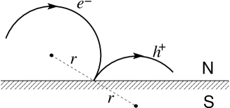
Figure 10: Andreev reflected orbit. The mapping from one center to the following one is a point reflection.

Numerical results show that for magnetic fields $B>B_{c,1}$ there are only trajectories with an even number of collisions with the superconducting antidot, yielding vanishing transport coefficients $T_{h}$ and $R_{h}$. In order to derive the first critical field it is helpful to consider the mapping of the guiding centers of the trajectory arcs in the presence of Andreev reflection. Fig. 10 shows two segments of an orbit right before and right after a collision with the NS-interface. The center of the second arc can be constructed from the center of the first one via point reflection at the collision point at the NS-interface.

Consider one segment of an orbit with radius $r$ reaching from the outer wall to the antidot. The distance between the center of this arc and the outer wall has to be less than $r$ and the same holds for the distance between the center and the antidot. This means that the center has to be inside the shaded area shown in Fig. 11. Consider an orbit that hits the superconductor only once. Such an orbit has to reach from the outer wall to the antidot and back to the wall. So the centers before and after the Andreev reflection have to be located inside the shaded area. This condition is easiest to fulfill for an orbit that has its center at one midpoint of the inner quadratic boundary, as shown in Fig. 11. The question is if for a certain radius the center after the Andreev reflection can no longer be mapped into the shaded region.

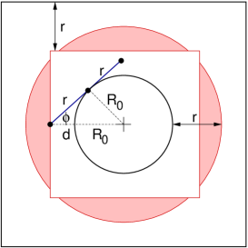
Figure 11: The shaded area shows all possible locations for centers of orbits that connect the outer walls with the antidot.

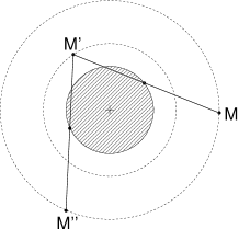
Figure 12: $M$ is the center of the first arc before the Andreev reflection. After one Andreev reflection it is mapped to $M^{\prime}$, after another one it is mapped to $M^{\prime\prime}$, which has the same distance from the center of the antidot as $M$.

The distance $d$ between the antidot and the inner square is $d=L/2-r-R_{0}$, where L is the side length of the square cavity and $R_{0}$ is the radius of the antidot. Applying the cosine-theorem to the triangle shown in Fig. 11 we get $R_{0}^{2}=r^{2}+(R_{0}+d)^{2}-2r(R_{0}+d)\cos\phi$. So the angle $\phi$ can be written as

$$\cos\phi=\frac{L^{2}-4R_{0}^{2}+8r^{2}-4Lr}{4r(L-2R)}.$$ (5)

The distance between the final point and the central horizontal line is $y=2r\sin\phi=2r\sqrt{1-\cos^{2}\phi}$. In order to get only one single Andreev reflection, the final point has to be inside the shaded region, therefore we have to claim $y>R_{0}+d$, which means

$$2r\sqrt{1-\cos^{2}\phi}-\frac{L}{2}+r>0.$$ (6)

Solving this inequality for $L=5W$ and $R_{0}=W$ we find a critical radius $r_{c}=1.0505W$, which corresponds via $r/W=B_{0}/B$ to a critical field of

$$B_{c,1}=0.9519B_{0}\,.$$ (7)

Up to now we have only shown that for a magnetic field $B>B_{c,1}$ the particles hit the superconductor at least twice consecutively. But now it is easy to see that the number of Andreev reflections is indeed even. Two Andreev reflections in a row correspond to a rotation of the center around the center of the antidot, as shown in Fig. 12. After an even number of Andreev reflections the center of the arc is always located on the outer dashed circle, which has a radius greater than $R_{0}+d$. After an odd number of reflections at the superconductor it is on the inner dashed circle with a radius smaller than $R_{0}+d$. Therefore the particle can only ‘escape’ the superconductor after an even number of collisions, which explains the fact.

References

- (1) K.-F. Berggren and S. Åberg (eds), QUANTUM CHAOS Y2K: Proceedings of Nobel Symposium 116, (World Scientific, 2000).
- (2) Y. Alhassid, Rev. Mod. Phys. 72, 895 (2000).
- (3) R. A. Jalabert in New Directions in Quantum Chaos, G. Casati, I. Guarneri, and U. Smilansky (eds) (IOS Press, Amsterdam, 2000).
- (4) K. Richter, Springer Tracts in Modern Physics 161, (Springer, Berlin, 2000).
- (5) I. Kosztin, D. L. Maslov, and P. M. Goldbart, Phys. Rev. Lett. 75, 1735 (1995).
- (6) For a recent review see, e.g., C. W. J. Beenakker, cond-mat/0406018.
- (7) J. Eroms, M. Tolkiehn, D. Weiss, U. Rössler, J. DeBoeck, and S. Borghs, Europhys. Lett. 58, 569 (2002).
- (8) A. F. Andreev, JETP 19, 1228 (1964)
- (9) J. Melsen, P. Brouwer, K. Frahm, and C. Beenakker, Europhys. Lett. 35, 7 (1996).
- (10) A. A. Clerk, P. W. Brouwer, and V. Ambegaokar, Phys. Rev. B 62, 10226 (2000).
- (11) W. Ihra, M. Leadbeater, J. L. Vega, and K. Richter, Eur. Phys. J. B 21, 425 (2001).
- (12) H. Schomerus and C. W. J. Beenakker, Phys. Rev. Lett. 82, 2951 (1999).
- (13) D. Taras-Semchuk and A. Altland, Phys. Rev. B 64, 014512 (2001).
- (14) J. Cserti, P. Polinák, G. Palla, U. Zülicke, and C. J. Lambert, Phys. Rev. B 69, 134514 (2004).
- (15) G. Fagas, G. Tkachov, A. Pfund, and K. Richter, Phys. Rev. B 71, 224510 (2005).
- (16) D. K. Ferry and S. M. Goodnick, Transport in Nanostructures (Cambridge University Press, 1997)
- (17) J. B. Ketterson and S. N. Song, Superconductivity (Cambridge University Press, 1999).
- (18) F. Taddei, S. Sanvito, J. H. Jefferson, and C. J. Lambert, Phys. Rev. Lett. 82, 4938 (1999).
- (19) C. J. Lambert, V. C. Hui, and S. J. Robinson, J. Phys.: Cond. Mat. 5, 4187 (1993).
- (20) P. Gaspard and J. R. Dorfman, Phys. Rev. E 52, 3525 (1995).
- (21) Z. Kovács, Phys. Rep. 290, 49 (1997).
- (22) L. G. G. V. Dias Da Silva and M. A. M. de Aguiar, Eur. Phys. J. B 16, 719 (2000).
- (23) M. Fliesser, G. J. O. Schmidt, and H. Spohn, Phys. Rev. E 53, 5690 (1996).
- (24) A. S. Sachrajda et al., Phys. Rev. Lett. 80, 1948 (1998).
- (25) In a strict sense, there is no chaos since all trajectories remain in the cavity for a finite time only.
- (26) K. Richter and M. Sieber, Phys. Rev. Lett. 89, 206801 (2002).
- (27) For a chaotic Andreev billiard one finds for the weak localization correction to the averaged conductance , where is the size of the interface with the superconductor and is the width of the leads attached, see: A. Lassl, diploma thesis, Universität Regensburg, unpublished, 2003.