Cluster approach study of intersite electron correlations in pyrochlore and checkerboard lattices

Abstract

To treat effects of electron correlations in geometrically frustrated pyrochlore and checkerboard lattices, an extended single-orbital Hubbard model with nearest neighbor hopping $\sim t$ and Coulomb repulsion $\sim V$ is applied. Infinite on-site repulsion, $U\to\infty$, is assumed, thus double occupancies of sites are forbidden completely in the present study. A variational Gutzwiller type approach is extended to examine correlations due to short-range $V-$interaction and a cluster approximation is developed to evaluate a variational ground state energy of the system. Obtained analytically in a special case of quarter band filling appropriate to LiV₂O₄, the resulting simple expression describes the ground state energy in the regime of intermediate and strong coupling $V$. Like in the Brinkman-Rice theory based on the standard Gutzwiller approach to the Hubbard model, the mean value of the kinetic energy is shown to be reduced strongly as the coupling $V$ approaches a critical value $V_{c}$. This finding may contribute to explaining the observed heavy fermion behavior in LiV₂O₄.

I Introduction

The pyrochlore lattice is a three-dimensional network of corner-sharing tetrahedra formed by B-cations in pyrochlore oxides A₂B₂O₇, in cubic spinel oxides AB₂O₄ and in cubic Laves-phase intermetallic compounds AB₂. These compounds exhibit a wide variety of physical properties ranging from magnetic insulator through bad metal to superconductor with relatively high transition temperature. One of the most spectacular properties in this family of $d$-systems is the heavy fermion (HF) behavior found in LiV₂O₄ and Y(Sc)Mn₂ at low temperatures. Kondo97 ; Wada87 ; Fisher92 To understand the nature of HF quasiparticles in Y(Sc)Mn₂, it was suggested Isoda00 ; Fujimoto01 that effects of geometrical frustration on the itinerant electron system in the pyrochlore lattice are of crucial importance.

In fact, in the pyrochlore lattice with a single orbital on each site, a special lattice geometry manifests itself through a flat band on the top of the dispersive one-particle electron spectrum.Isoda00 In the half-filled case, the Fermi level touches the flat band singularity from below. In actual band structure calculations of a multi-orbital $d$-system, this singularity is removed and, instead, a sharply peaked feature in the density of states is seen. By treating the problem of Y(Sc)Mn₂ within a single band pyrochlore Hubbard model in a weak correlation limit and assuming proximity of the Fermi level to the peaked feature in the density of states, the authors Isoda00 ; Fujimoto01 suggested a new scenario for the HF-like behavior of the frustrated system. In contrast, in LiV₂O₄ the mean occupancy of the $V$-ion $d$-shell equals 1.5 and corresponds to the quarter-filling of the almost three-fold degenerate $t_{2g}$ band.Singh99 Therefore, in this compound the Fermi level is pushed down strongly from the ’flat-band’ peculiarity and the above arguments for the HF quasiparticle formation are not applicable any more. In this respect, even by taking into account strong on-site Coulomb correlation effects, not included in the band structure calculations, one cannot cure the situation.

Several scenarios for explaining HF properties in LiV₂O₄, including the one based on multi-component fluctuationsYamashita03 , are proposed in the literature and reviewed briefly in Ref.Fulde03, . While the strong on-site Coulomb interaction $\sim U$ is incorporated necessarily in most of these scenarios, effects of inter-site Coulomb correlations on the HF properties in the pyrochlore lattice have been studied much less. The latter effects in the form of Anderson’s ’tetrahedron rule’ Anderson56 are used explicitly in Ref.Fulde01, to build a physical picture of low temperature properties in LiV₂O₄. According to this picture, Coulomb repulsions of electrons on nearest neighbor sites suppress charge fluctuations appreciably and a state of slowly fluctuating and nearly decoupled chain-like and ring configurations of spins $s=1/2$ is formed to give a large low temperature spin entropy. However, the mechanism for suppressing charge fluctuations in the pyrochlore lattice has not been elaborated in detail.

In the present paper, we address this problem and concentrate on the study of charge degrees of freedom and their possible role in forming heavy quasiparticles. For this purpose, the potentially important role of inter-site electron Coulomb interaction in the pyrochlore lattice is emphasized in a particular case of quarter band filling appropriate to LiV₂O₄. We use an extended single-orbital Hubbard model composed of the kinetic term with a tight-binding nearest neighbor (n.n.) hopping amplitude $t$, strong Hubbard term $\sim U$ and Coulomb term describing n.n. electron repulsion $\sim V$ of variable strength with respect to $t$. In spite of its serious simplification, this minimal model is believed to capture generic effects of strong inter-site Coulomb correlations inherent to more realistic pyrochlore electronic models including several $d$-orbitals on each lattice site. Noting that $U$ is the largest energy parameter, we simply put $U\rightarrow\infty$ in our calculations. At $U\rightarrow\infty$ and far away from half-filling, one expects the system to be in a metallic state at weak coupling $V$. Our aim is to show that in the strong coupling limit, $V\gg t$, an effective electron bandwidth in the quarter-filled system can be strongly reduced due to short-range charge correlations. This regime of a strongly correlated metal can be understood as a state of almost localized electrons.

Short-range spin correlations are neglected here because the limit $U\rightarrow\infty$ is assumed. Instead, we concentrate completely on the problem of short-range charge correlations which are believed to provide the dominant mechanism for strong suppression of the electron kinetic motion in the pyrochlore lattice and, therefore, may contribute to the heavy quasiparticle formation.

To conclude this Section, we outline briefly the structure of the paper and the method used. We extend the Gutzwiller variational approach to a form that allows us to treat the inter-site correlation problem. For completeness, we involve in our consideration also the 2D checkerboard lattice which is a planar analogue of the 3D pyrochlore lattice. Our method is applicable equally to both cases and relies on a cluster character of the pyrochlore (checkerboard) lattice structure, which means that each tetrahedron (plaquette) is regarded as an elementary entity. In Section II, the underlying electronic model is defined and rewritten in a cluster representation. The ground state variational wave function of the interacting system is constructed by applying to the system of noninteracting electrons two kinds of projectors. The first is the Gutzwiller projector taken in the limit $U\rightarrow\infty$ to eliminate double occupancy of sites. The second projector is defined in terms of cluster occupancy operators in such a way that the weights of different charge configurations in each cluster are controlled by a correlation strength parameter $\eta$ which is the only variational parameter in our theory.

In Section III, a variational ground state energy functional is defined and a factorization procedure of its approximate calculation is discussed in detail. Within this context, the concept of the basic cluster in the pyrochlore (checkerboard) lattice is introduced and a mechanism for suppressing of inter-cluster charge fluctuations is explained. In Section IV, the calculations are performed and the resulting ground state energy as a function of the coupling $V$ is analyzed. This analysis shows that the mean kinetic energy in the system is strongly renormalized and tends to zero as $V$ approaches some critical value $V_{c}$. Also, our variational theory suggests, that electron localization transition occurs at $V=V_{c}$, and for $V>V_{c}$ the electrons are in a fully localized insulating state for which quantum charge fluctuations are completely missed. The results are discussed in Section V. By drawing a close analogy with the Brinkman-Rice localization transition predicted in the variational studyBrinkman70 of the standard Hubbard model, we argue that improper description of the actual metal-insulator transition does not invalidate our cluster variational theory in all respects. In particular, the theory is still valid in describing a metallic strongly correlated (the not yet localized) regime for $V\lesssim V_{c}$. Concluding remarks can be also found in Section V.

II Model formulation and trial wave function

Let us start with an extended single-orbital Hubbard model in the pyrochlore or checkerboard lattice

$$H=-t\sum_{<ij>,\sigma}\left(c^{\dagger}_{i\sigma}c_{j\sigma}+c^{\dagger}_{j\sigma}c_{i\sigma}\right)+V\sum_{<ij>}n_{i}n_{j}+U\sum_{i}n_{i\uparrow}n_{i\downarrow},$$ (1)

where the summation in the first two terms is taken over the n.n. sites, each pair $<ij>$ is counted once; $c^{\dagger}_{i\sigma}(c_{j\sigma})$ is the creation (annihilation) electron operator with spin $\sigma=\uparrow,\downarrow$ and $n_{i}=\sum_{\sigma}c^{\dagger}_{i\sigma}c_{i\sigma}$. We are interested in the model regime far away from the band half-filling in the limit $U\to\infty$.

Let us consider a plaquette in the checkerboard or a tetrahedron in the pyrochlore lattices as an elementary $\mathcal{K}$-th cluster, each contains four sites numbered as $k=1,...,4$. Each lattice site belongs to two clusters and thus the neighboring clusters overlap. If $L$ is the number of the lattice sites, then $L/2$ is the number of overlapping clusters, i.e. ${\mathcal{K}}=1,2,\ldots,L/2$. Now, the first two terms in the Hamiltonian (1) can be rewritten in the cluster representation

$$H_{t-V}=\sum_{{\mathcal{K}}=1}^{L/2}H_{\mathcal{K}},\qquad H_{\mathcal{K}}=T_{\mathcal{K}}+V_{\mathcal{K}},$$

$$T_{\mathcal{K}}=-t\sum_{\stackrel{{\scriptstyle k\neq k^{\prime}}}{{(k,k^{\prime})\in{\mathcal{K}}}}}\sum_{\sigma}c^{\dagger}_{k\sigma}c_{k^{\prime}\sigma},$$ (2)

$$V_{\mathcal{K}}=\frac{V}{2}\sum_{\stackrel{{\scriptstyle k\neq k^{\prime}}}{{(k,k^{\prime})\in{\mathcal{K}}}}}n_{k}n_{k^{\prime}},\qquad n_{k}=\sum_{\sigma}c^{\dagger}_{k\sigma}c_{k\sigma}.$$

Since $U\to\infty$, the double occupancy of sites is forbidden and the unit operator on each $k$-th site is

$$1_{k}=P_{k}(0)+P_{k}(1),$$

$$P_{k}(0)=(1-n_{k\uparrow})(1-n_{k\downarrow}),$$ (3)

$$P_{k}(1)=\sum_{\sigma=\uparrow,\downarrow}P_{k\sigma}(1),\qquad P_{k\sigma}=n_{k\sigma}(1-n_{k\bar{\sigma}}),$$

where $P_{k}(0)$ and $P_{k}(1)$ are the projection operators onto the empty and singly occupied $k$-th site states, respectively; $\bar{\sigma}=-\sigma$. Further, to distinguish cluster states with occupancies $n=0,\ldots,4$, we define the cluster projection operators

$${\mathcal{P}}_{\mathcal{K}}(0)=\prod_{k=1}^{4}{\mathrm{P}}_{k}(0),$$

$${\mathcal{P}}_{\mathcal{K}}(1)=\sum_{k=1}^{4}{\mathrm{P}}_{k}(1)\left[\prod_{k^{\prime}\neq k}{\mathrm{P}}_{k^{\prime}}(0)\right],$$

$${\mathcal{P}}_{\mathcal{K}}(2)=\sum_{k<k^{\prime}}{\mathrm{P}}_{k}(1){\mathrm{P}}_{k^{\prime}}(1)\left[\prod_{k^{\prime\prime}\neq k,k^{\prime}}{\mathrm{P}}_{k^{\prime\prime}}(0)\right],$$ (4)

$${\mathcal{P}}_{\mathcal{K}}(3)=\sum_{k=1}^{4}{\mathrm{P}}_{k}(0)\left[\prod_{k^{\prime}\neq k}{\mathrm{P}}_{k^{\prime}}(1)\right],$$

$${\mathcal{P}}_{\mathcal{K}}(4)=\prod_{k=1}^{4}{\mathrm{P}}_{k}(1),$$

where ${(k,k^{\prime},k^{\prime\prime})\in{\mathcal{K}}}$ is implied. Disregarding the spins, we note that the configurational space of a cluster contains in total 16 allowed charge configurations. For instance, the occupancy state $n=2$ is composed of 6 configurations. Taking into account the frustration of the system, we suggest that the basic operators (4) and the associated cluster occupancies in the lattice suffice to capture the correlated metallic regime of the model, as suggested by the form (6) of $V_{\mathcal{K}}$ term below.

In terms of the projection operators (4), the kinetic and the Coulomb terms in (2) can be presented as follows

$$T_{\mathcal{K}}=\sum_{n=1}^{3}T_{\mathcal{K}}(n)=\sum_{n=1}^{3}{\mathcal{P}}_{\mathcal{K}}(n)T_{\mathcal{K}}{\mathcal{P}}_{\mathcal{K}}(n),$$ (5)

$$V_{\mathcal{K}}=V\left[{\mathcal{P}}_{\mathcal{K}}(2)+3{\mathcal{P}}_{\mathcal{K}}(3)+6{\mathcal{P}}_{\mathcal{K}}(4)\right],$$ (6)

where the diagonal form of $T_{\mathcal{K}}$ occurs because any electron hopping within a cluster does not change its charge occupancy. Finally, we define the cluster number operator $N_{\mathcal{K}}=\sum_{k\in{\mathcal{K}}}n_{k}$, and note that the mean value $\langle N_{\mathcal{K}}\rangle=2$ corresponds to the quarter band filling.

A trial ground state wave function of the interacting system is constructed below in two steps. First, in the limit $V=0$, we introduce the Gutzwiller projected Fermi sea $(U\to\infty)$:

$$|\psi\rangle_{V=0}=\frac{1}{\sqrt{\Omega}}\prod_{k=1}^{L}\left[1-n_{k\uparrow}n_{k\downarrow}\right]|\Phi_{0}\rangle\equiv|\psi_{0}\rangle,$$ (7)

where $|\Phi_{0}\rangle$ is a single Slater determinant describing a metallic state for $N=L/2$ noninteracting electrons; $\Omega$ is the norm. Since the system is away from half-filling, the Gutzwiller projectors Gutzwiller65 ; Vollhardt84 in (7) are expected to lead to a moderate renormalization of metallic properties. A regime of strongly correlated metal at quarter band filling may occur in an interacting system with strong inter-site Coulomb repulsion $V$.

To take into consideration electron correlations due to $V\neq 0$, we define below a product of generalized Gutzwiller projectors $G_{\mathcal{K}}(\eta)$ acting in the occupancy space of the $\mathcal{K}$-th clusters (${\mathcal{K}}=1,2,\ldots,L/2$); here $\eta$ is the variational parameter varying in the range $0\leq\eta\leq 1$. To justify the proper choice of $G_{\mathcal{K}}(\eta)$, let us start with the limit of extreme coupling, $V/t\to\infty$. In this limit, the ground state cluster charge configurations are those obeying the ’tetrahedron rule’, i.e. each cluster is occupied strictly with two electrons, and the ground state energy is $V$ per cluster. Therefore, $G_{\mathcal{K}}(\eta)={\mathcal{P}}_{\mathcal{K}}(2)$ and our convention is that $\eta=0$ in this limit. At finite $t$, electron hopping processes create exited charge configurations of higher, $n=3,4$ and lower, $n=0,1$, cluster occupancies. To ascribe optimal weights to the exited configurations, we use the following prescription. Consider first a pair of clusters, ${\mathcal{K}}_{1}$ and ${\mathcal{K}}_{2}$, occupied with $n_{1}=1$ and $n_{2}=3$ electrons. By noting that the potential energy of such a fluctuation is $3V$, which exceeds the energy $2V$ of the dominant configuration of two electrons per cluster by $V$, we ascribe to it a weight factor $\eta\leq 1$. The cost of the potential energy of the more extreme charge fluctuation of a pair of clusters, i.e. $n_{1}=0$ and $n_{2}=4$, is $4V$, and therefore we associate the weight factor ${\eta}^{4}$ with this fluctuation. More complex many-cluster excited charge configurations can be easily recognized to be combinations of the elementary ones discussed above. These observations are comprised in the following form of a generalized cluster Gutzwiller projector

$$G_{\mathcal{K}}(\eta)={\eta}^{2}{\mathcal{P}}_{\mathcal{K}}(0)+\sqrt{\eta}{\mathcal{P}}_{\mathcal{K}}(1)+{\mathcal{P}}_{\mathcal{K}}(2)+\sqrt{\eta}{\mathcal{P}}_{\mathcal{K}}(3)+{\eta}^{2}{\mathcal{P}}_{\mathcal{K}}(4),$$ (8)

and of a trial ground state wave function defined as

$$|\psi(\eta)\rangle=\prod_{\mathcal{K}}^{L/2}G_{\mathcal{K}}(\eta)|\psi_{0}\rangle=|\psi\rangle,$$ (9)

where $0\leq\eta\leq 1$. If $\eta=1$, the projector $G_{\mathcal{K}}(\eta)$ becomes the unity operator, which corresponds to the limit of zero coupling, $V=0$.

Note, the form (8) of a generalized Gutzwiller projector and, hence, the trial wave function (9) are inspired by the form (6) of $V_{\mathcal{K}}$ term and Anderson’s reasoning Anderson56 on a macroscopical degeneracy of the ground state charge configurations in the limit of the extreme coupling, $V/t\to\infty$. We expect the wave function ansatz (9) to be valid down to intermediate coupling values $V\sim zt$, where $z=6$ is the pyrochlore (checkerboard) lattice coordination number. It is much less appropriate in the limit of a weak coupling $V\lesssim t$, where the kinetic energy effects become dominant and the arguments based on the potential energy counting only are not sufficient.

III Variational ground state energy and factorization procedure

With definitions (1) and (2), the ground state energy of the lattice system ${\mathcal{E}}(\eta)=\langle\psi|H|\psi\rangle/\langle\psi|\psi\rangle$ can be written as a sum of cluster energies

$${\mathcal{E}}(\eta)=\frac{L}{2}E(\eta);\qquad E(\eta)=\frac{\langle\psi(\eta)|H_{\mathcal{K}}|\psi(\eta)\rangle}{\langle\psi(\eta)|\psi(\eta)\rangle},$$ (10)

where the translational invariance of the wave function (9), i.e. $\langle\psi|H_{\mathcal{K}}|\psi\rangle=\langle\psi|H_{\mathcal{K}^{\prime}}|\psi\rangle$ for ${\mathcal{K}}\neq{\mathcal{K}^{\prime}}$, is taken into account. From now on, the expectation energy value calculation reduces to a local problem.

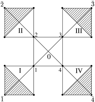
Figure 1: Fragment of the checkerboard lattice chosen to be a minimal basic cluster in the variational cluster calculations. Each label ${\mathcal{K}}$ of side clusters $(\mathrm{I},\ldots,\mathrm{IV})$ is a composite one, ${\mathcal{K}}=(k,\overline{k})$, where $k$ ($=1,...,4$) is referred to a site shared with the central 0-cluster and $\overline{k}$ ($=\overline{1},...,\overline{4}$) is for the complementary 3-site fragment (hatched). In the pyrochlore lattice, the same labelling is used for a minimal basic cluster formed by five corner-sharing tetrahedra.

To evaluate $E(\eta)$, an approximate procedure is developed and applied below . The starting point is to divide the lattice into two parts. The smaller one, which is refereed below to as the basic cluster ($bc$), contains five connected elementary clusters, as explained in Fig.1 for the checkerboard lattice. According to this picture, the same hopping parameter $t$ and Coulomb interaction constant $V$ should be ascribed to the horizontal, vertical and diagonal bonds (linear segments) connecting neighboring lattice sites. One can easily realize that the basic cluster in Fig.1 has its 3D counterpart formed by five corner-sharing tetrahedra in the pyrochlore lattice, the former being a planar projection of the latter. Therefore, both cases can be treated on an equal footing. With this division, we suggest that the essential effects of the local interactions involved in $E(\eta)$ are captured by a basic cluster.

Below, a factorization procedure for the trial wave function (9) is used, which reduces the calculation of expectation value $E(\eta)$ from the lattice to a basic cluster. In the present study, we take advantage of another simplifying assumption which amounts to the neglect of the spatial charge correlations in the starting wave function (7). Such an approximation is inherent also to the Gutzwiller approach study of standard Hubbard model. Actually, as shown in Ref.Ogata75, , when calculating the hopping matrix elements (the interacting $U$-term is accounted for exactly) in the $N$-particle state $|\Phi_{0}\rangle$ of noninteracting electrons, the neglect of the configuration dependence at this stage is equivalent to all assumptions made by Gutzwiller Gutzwiller65 and leads to an identical result.Ogata75 The approximation is controlled by the parameter $1/z$, where $z$ is the lattice coordination number; it gives an exact result in the limit of infinite spatial dimension and requires only very small corrections for three-dimensional lattices.Vollhardt84 ; Metzner88 Though the wave function (7) describes an electron system with extremely strong on-site repulsion, we expect that foregoing arguments are still valid provided the electron concentration is sufficiently far away from the half filled band case.

After explaining the very essence of the approximation chosen to calculate the expectation energy value $E(\eta)$, we proceed now with its evaluation. First, a basic cluster is selected as a lattice fragment composed of a central elementary $0$-cluster whose four sites are shared with four (I,…,IV) side elementary clusters, as depicted in Fig.1. From now on, the trial state (9) can be written in the following form

$$|\psi(\eta)\rangle=G_{{\mathcal{K}}_{0}}(\eta)G_{\left\{{\mathcal{K}}\right\}}(\eta)G_{\left\{{\mathcal{K}^{\prime}}\right\}}(\eta)|\psi_{0}\rangle,$$ (11)

where $G_{{\mathcal{K}}_{0}}$ is referred to the central $0$-cluster, $G_{\left\{{\mathcal{K}}\right\}}=\prod_{{\mathcal{K}}=I}^{IV}G_{\mathcal{K}}$ is for four side clusters and $G_{\left\{{\mathcal{K}^{\prime}}\right\}}=\prod_{{\mathcal{K}^{\prime}}(\neq{{\mathcal{K}}_{0},{\mathcal{K}}})}G_{\mathcal{K}^{\prime}}$ is for the remaining system. The factorization procedure now reads as follows

$$E(\eta) \simeq \frac{\langle\psi_{0}|G_{\left\{{\mathcal{K}}\right\}}G_{{\mathcal{K}}_{0}}H_{{\mathcal{K}}_{0}}G_{{\mathcal{K}}_{0}}G_{\left\{{\mathcal{K}}\right\}}|\psi_{0}\rangle\langle\psi_{0}|G^{2}_{\left\{{\mathcal{K}^{\prime}}\right\}}|\psi_{0}\rangle}{\langle\psi_{0}|G^{2}_{\left\{{\mathcal{K}}\right\}}G^{2}_{\left\{{{\mathcal{K}}_{0}}\right\}}|\psi_{0}\rangle\langle\psi_{0}|G^{2}_{\left\{{\mathcal{K}^{\prime}}\right\}}|\psi_{0}\rangle}=$$ (12)

$$= \frac{\langle\psi_{0}|G_{\left\{{\mathcal{K}}\right\}}G_{{\mathcal{K}}_{0}}H_{{\mathcal{K}}_{0}}G_{{\mathcal{K}}_{0}}G_{\left\{{\mathcal{K}}\right\}}|\psi_{0}\rangle}{\langle\psi_{0}|G^{2}_{\left\{{\mathcal{K}}\right\}}G^{2}_{\left\{{{\mathcal{K}}_{0}}\right\}}|\psi_{0}\rangle}=\frac{\langle\psi_{bc}|H_{{\mathcal{K}}_{0}}|\psi_{bc}\rangle}{\langle\psi_{bc}|\psi_{bc}\rangle},$$

where the trial state $|\psi_{bc}\rangle$ in the cluster approximation is taken in the form

$$|\psi_{bc}(\eta)\rangle=G_{{\mathcal{K}}_{0}}(\eta)G_{\left\{{\mathcal{K}}\right\}}(\eta)|\psi_{0}\rangle,$$ (13)

and the labelling bc is due to a distinguished basic cluster either in the pyrochlore or in the checkerboard lattice. Both, three- and two-dimensional basic clusters have the same lattice connectivity and, therefore, in our study are treated equally. We believe that the basic cluster chosen is inevitably a minimal one for the present problem. This means that it could not be reduced further, for instance, to the size of 4-site elementary cluster, otherwise the most important correlation effect of the kinetic energy reduction would be lost. Actually, when calculating $\langle\psi_{bc}|T_{{\mathcal{K}}_{0}}|\psi_{bc}\rangle/\langle\psi_{bc}|\psi_{bc}\rangle/=\langle T_{{{\mathcal{K}}_{0}}}\rangle_{bc}$, one finds that the electron hopping processes involved in $T_{{\mathcal{K}}_{0}}$ do not change an occupancy of the ${\mathcal{K}}_{0}$ -th cluster, but any of them changes simultaneously occupation numbers of a pair of side clusters. As a result, the side cluster charges deviate from their mean value $n=2$. With increasing coupling constant $V$, however, the cluster states of high, $n=3,4$ and low, $n=0,1$, occupancies are suppressed, and thus the hopping processes within the ${\mathcal{K}}_{0}$-th cluster are hampered. As a consequence, the expectation value of the kinetic term $\langle T_{{{\mathcal{K}}_{0}}}\rangle_{bc}$ is reduced strongly in a way similar to that found in the standard Hubbard model treated within the Gutzwiller approximation. In the latter case, a minimal basic cluster is 2-site one as suggested by Razafimandimby. Raz82

In order to facilitate evaluation of $E(\eta)$, we resort to a new diagonal form of the operator product $G_{{\mathcal{K}}_{0}}G_{\{{\mathcal{K}}\}}$ with respect to the occupancy number $n$ of the central cluster ${\mathcal{K}}_{0}$. For this purpose, let us consider side clusters ${\mathcal{K}}=\mathrm{I},\ldots,\mathrm{IV}$ and their labels $\mathcal{K}$ as composite ones, ${\mathcal{K}}=(k,\overline{k})$, for instance, $\mathrm{I}=(1,\overline{1})$, etc. Here $k$ denotes a site common both to the $\mathcal{K}$-th and the central ${\mathcal{K}}_{0}$ clusters, while $\overline{k}$ refers to the complementary 3-site fragment of the ${\mathcal{K}}-$th side cluster, as shown in Fig.  1. For the $\overline{k}-$th fragment, let $|\overline{k},m\rangle$ be a quantum state with an electron occupancy $m(=0,..,3)$ and ${\mathcal{P}}_{\overline{k}}(m)=|\overline{k},m\rangle\langle\overline{k},m|$ are the corresponding projection operators. In terms of ${\mathcal{P}}_{\overline{k}}(m)$, the projection operators ${\mathcal{P}_{\mathcal{K}}}(n)$ of side $\mathcal{K}$-clusters can be now written in a split form ${\mathcal{P}_{\mathcal{K}}}(n)=P_{k}(0){\mathcal{P}}_{\overline{k}}(n)+P_{k}(1){\mathcal{P}}_{\overline{k}}(n-1)$, with the convention ${\mathcal{P}}_{\overline{k}}(-1)={\mathcal{P}}_{\overline{k}}(4)=0$ assumed. With this redefinition of ${\mathcal{P}}_{\mathcal{K}}(n)$, the projectors $G_{\mathcal{K}}$ of side clusters are also split in two terms, each selecting one of two possible occupancies, $n=0,1$, of the $k-$th site common to a given $\mathcal{K}$ and the central ${\mathcal{K}}_{0}$ clusters:

$$G_{\mathcal{K}}(\eta)=P_{k}(0)Q_{\overline{k}}(\eta)+P_{k}(1)R_{\overline{k}}(\eta).$$ (14)

Here $Q_{\overline{k}}$ and $R_{\overline{k}}$ operate in the charge configuration space of the $\overline{k}-$th fragment

$$Q_{\overline{k}}(\eta) = {\eta}^{2}{\mathcal{P}}_{\overline{k}}(0)+\sqrt{\eta}{\mathcal{P}}_{\overline{k}}(1)+{\mathcal{P}}_{\overline{k}}(2)+\sqrt{\eta}{\mathcal{P}}_{\overline{k}}(3),$$

$$R_{\overline{k}}(\eta) = \sqrt{\eta}{\mathcal{P}}_{\overline{k}}(0)+{\mathcal{P}}_{\overline{k}}(1)+\sqrt{\eta}{\mathcal{P}}_{\overline{k}}(2)+{\eta}^{2}{\mathcal{P}}_{\overline{k}}(3).$$ (15)

with the following obvious properties, $Q^{2}_{\overline{k}}(\eta)=Q_{\overline{k}}(\eta^{2})$ and $R^{2}_{\overline{k}}(\eta)=R_{\overline{k}}(\eta^{2})$.

It is not a difficult task to rewrite the operators ${\mathcal{P}}_{\overline{k}}(m)$ and their linear combinations (15) through the site projection operators (3), which is useful for further calculations. The weight factors in (15) serve as a measure of the correlation strength in dependence on the $\overline{k}-$th fragment charge occupancy. Finally, we use the definition (8) for $G_{{\mathcal{K}}_{0}}$ and the presentation (14) for $G_{\mathcal{K}}$ to write down the following form of the product $G_{{\mathcal{K}}_{0}}G_{\{{\mathcal{K}}\}}$:

$$G_{{\mathcal{K}}_{0}}(\eta)G_{\{{\mathcal{K}}\}}(\eta)=\sum_{n=0}^{4}f_{n}(\eta)X(n;\eta),$$ (16)

where weight factors $f_{n}(\eta)$ are found to be $f_{0}=f_{4}={\eta}^{2},f_{1}=f_{3}=\sqrt{\eta},f_{2}=1$, and the operators $X(n;\eta)$ discriminate the basic cluster charge configurations in accord with the central cluster occupancy $n$:

$$X(0;\eta) = \prod_{k=1}^{4}P_{k}(0)Q_{\overline{k}}(\eta),$$

$$X(1;\eta) = \sum_{k=1}^{4}P_{k}(1)R_{\overline{k}}(\eta)\prod_{k^{\prime}\neq k}^{4}P_{k^{\prime}}(0)Q_{\overline{k^{\prime}}}(\eta),$$ (17)

$$X(2;\eta) = \sum_{k<k^{\prime}}P_{k}(1)P_{k^{\prime}}(1)R_{\overline{k}}(\eta)R_{\overline{k^{\prime}}}(\eta)\prod_{k^{\prime\prime}\neq k,k^{\prime}}P_{k^{\prime\prime}}(0)Q_{\overline{k^{\prime\prime}}}(\eta),$$

$$X(3;\eta) = \sum_{k=1}^{4}P_{k}(0)Q_{\overline{k}}(\eta)\prod_{k^{\prime}\neq k}^{4}P_{k^{\prime}}(1)R_{\overline{k^{\prime}}}(\eta),$$

$$X(4;\eta) = \prod_{k=1}^{4}P_{k}(1)R_{\overline{k}}(\eta).$$

The factorization procedure (12) constitutes the first step of our approximation for calculating the expectation energy value $E(\eta)$. As mentioned before, the second approximation consists in the neglect of electron spatial correlations within the Gutzwiller projected Fermi sea state $|\psi_{0}\rangle=|\psi\rangle_{V=0}$, Eq.(7). For instance, when having a two-site electron density correlation function $\langle\psi_{0}|n_{k,\sigma}n_{k^{\prime},\sigma^{\prime}}|\psi_{0}\rangle$, we decouple it as follows $(k\neq k^{\prime})$:

$$\langle\psi_{0}|n_{k,\sigma}n_{k^{\prime},\sigma^{\prime}}|\psi_{0}\rangle\simeq\langle\psi_{0}|n_{k,\sigma}|\psi_{0}\rangle\langle\psi_{0}|n_{k^{\prime},\sigma^{\prime}}|\psi_{0}\rangle=\left(\frac{1}{2}n\right)^{2}$$ (18)

where $n=N/L$ is an electron concentration and the extra factor 1/2 in the right-hand side is due to spatially uncorrelated electron spins. Since doubly occupied sites are forbidden, $\langle\psi_{0}|n_{k,\uparrow}n_{k,\downarrow}|\psi_{0}\rangle=0$, in terms of site projection operators (3), the decoupling (18) reads $(k\neq k^{\prime})$:

$$\langle\psi_{0}|P_{k}(n)P_{k^{\prime}}(n^{\prime})|\psi_{0}\rangle\simeq\langle P_{k}(n)\rangle_{0}\langle P_{k^{\prime}}(n^{\prime})\rangle_{0},$$ (19)

where $\langle P_{k}(n)\rangle_{0}=\langle\psi_{0}|P_{k}(n)|\psi_{0}\rangle=1/2(\delta_{n,0}+\delta_{n,1})$. Multi-site density correlation functions are decoupled in the same manner.

To complete this Section, let us calculate the norm

$$\langle\psi_{bc}(\eta)|\psi_{bc}(\eta)\rangle=\sum_{n=0}^{4}f^{2}_{n}(\eta)\langle X(n;\eta^{2})\rangle_{0},$$ (20)

where the average $\langle...\rangle_{0}$ is over the state $|\psi_{0}\rangle$.

By using the approximation (18) and (19) for a given electron concentration $n=1/2$, one finds an intermediate result

$$\langle X(n;\eta^{2})\rangle_{0}=\left(\frac{1}{2}\right)^{4}C^{4}_{n}\left(\langle Q(\eta^{2})\rangle_{0}\right)^{4-n}\left(\langle R(\eta^{2})\rangle_{0}\right)^{n},$$ (21)

where $C_{n}^{4}$ is a binomial and both $\langle Q_{\overline{k}}\rangle_{0}$ and $\langle R_{\overline{k}}\rangle_{0}$ are calculated to be $\overline{k}-$independent expectation values $\langle Q(\eta^{2})\rangle_{0}=\langle R(\eta^{2})\rangle_{0}=({\eta}^{4}+4{\eta}+3)/8$.

From Eq.(20), the norm can be now written as

$$\langle\psi_{bc}|\psi_{bc}\rangle=\left[\frac{{\eta}^{4}+4{\eta}+3}{8}\right]^{5}.$$ (22)

IV Calculation of the variational energy

We start with the evaluation of an expectation value of the Coulomb energy. Since the procedure is similar to that used in the previous Section, we present the resulting expression for the mean interaction energy per cluster

$$\frac{\langle\psi_{bc}|V_{{\mathcal{K}}_{0}}|\psi_{bc}\rangle}{\langle\psi_{bc}|\psi_{bc}\rangle} = 3V\frac{{\eta}^{4}+2{\eta}+1}{{\eta}^{4}+4{\eta}+3}=\left\{\begin{array}[]{l}\frac{3}{2}V,\quad\eta=1\\[8.53581pt] V,\quad\eta=0\end{array}\right.$$ (25)

Both limiting values in (25) can be easily understood on a general ground. Indeed, the value $(3/2)V$ corresponds to spatially uncorrelated electrons homogeneously distributed over the lattice, while the value $V$ is in compliance with any lattice charge configuration having two electrons within each elementary cluster.

The evaluation of the kinetic energy is much more involved. As a starting point, one has to rely on a general expression

$$\langle\psi_{bc}|T_{{\mathcal{K}}_{0}}|\psi_{bc}\rangle=-t\sum_{k\neq k^{\prime}}\sum_{\sigma}\langle c^{\dagger}_{k\sigma}c_{k^{\prime}\sigma}\rangle_{bc}=$$

$$=-t\sum_{k\neq k^{\prime}}\sum_{\sigma}\sum_{n=1}^{3}f^{2}_{n}\langle X(n;)c^{\dagger}_{k\sigma}c_{k^{\prime}\sigma}X(n;)\rangle_{0},$$ (26)

where each pair of sites $(k,k^{\prime})\in{\mathcal{K}}_{0}$ contributes equally to the sum (26); from now on we also use shortened notation $X(n;\eta)=X(n;)$. To make the calculation more transparent, we introduce projected fermionic operators $\tilde{c}^{\dagger}_{k\sigma}(\tilde{c}_{k\sigma})$ related to $c^{\dagger}_{k\sigma}(c_{k\sigma})$ as follows

$$\tilde{c}^{\dagger}_{k\sigma}=P_{k}(1)c^{\dagger}_{k\sigma}P_{k}(0),\qquad\tilde{c}_{k\sigma}=P_{k}(0)c_{k\sigma}P_{k}(1).$$ (27)

When operating in a space with no double site occupancy, $\tilde{c}^{\dagger}_{k\sigma}(\tilde{c}_{k\sigma})$ and $c^{\dagger}_{k\sigma}(c_{k\sigma})$ are equivalent.

Let us consider a particular pair $(k=1,k^{\prime}=2)$ and insert into (26) the explicit form of $X(n;)$ coming from (17). Then we obtain successively for $n=1,2,3$ the following intermediate form of hopping matrix elements

$$\langle X(1;)c^{\dagger}_{1\sigma}c_{2\sigma}X(1;)\rangle_{0}=$$

$$=\langle R_{\bar{1}}\tilde{c}^{\dagger}_{1\sigma}Q_{\bar{1}}\cdot Q_{\bar{2}}\tilde{c}_{2\sigma}R_{\bar{2}}\cdot P_{3}(0)Q^{2}_{\bar{3}}\cdot P_{4}(0)Q^{2}_{\bar{4}}\rangle_{0},$$

$$\langle X(2;)c^{\dagger}_{1\sigma}c_{2\sigma}X(2;)\rangle_{0}=$$ (28)

$$=\langle R_{\bar{1}}\tilde{c}^{\dagger}_{1\sigma}Q_{\bar{1}}\cdot Q_{\bar{2}}\tilde{c}_{2\sigma}R_{\bar{2}}\cdot\left[P_{3}(0)Q^{2}_{\bar{3}}\cdot P_{4}(1)R^{2}_{\bar{4}}+P_{3}(1)R^{2}_{\bar{3}}\cdot P_{4}(0)Q^{2}_{\bar{4}}\right]\rangle_{0},$$

$$\langle X(3;)c^{\dagger}_{1\sigma}c_{2\sigma}X(3;)\rangle_{0}=$$

$$=\langle R_{\bar{1}}\tilde{c}^{\dagger}_{1\sigma}Q_{\bar{1}}\cdot Q_{\bar{2}}\tilde{c}_{2\sigma}R_{\bar{2}}\cdot P_{3}(1)R^{2}_{\bar{3}}\cdot P_{4}(1)R^{2}_{\bar{4}}\rangle_{0}.$$

For brevity, in the above expressions we drop the arguments in $Q_{\bar{k}}(\eta)$ and $R_{\bar{k}}(\eta)$.

It is worth discussing shortly the physical content of expressions (28). An electron hopping within the central cluster is affected by its charge surrounding, which may occur in many configurations. In our description, all allowed configurations of the charge surrounding are comprised by a set of operators $Q_{\bar{k}}$ and $R_{\bar{k}}$ involved in the hopping matrix elements (28). This becomes more clear if one uses the explicit form of $Q_{\bar{k}}$ and $R_{\bar{k}}$, Eq.(15), which breaks up a hopping amplitude from (28) into a sum of terms, each of them corresponds to a particular configuration weighted with some $\eta-$dependent factor. In the uncorrelated limit, $\eta=1$, all these factors are unity, while for $\eta<1$ hopping amplitudes are suppressed due to short-range charge correlations.

The neglect of spatial electron correlations in $|\psi\rangle_{0}$ allows us to approximate the amplitudes (28) by using a decoupling procedure. For instance, the first expression in (28) is decoupled as follows

$$\langle X(1;)c^{\dagger}_{1\sigma}c_{2\sigma}X(1;)\rangle_{0}\simeq$$ (29)

$$\simeq \langle R_{\bar{1}}Q_{\bar{1}}\rangle_{0}\langle R_{\bar{2}}Q_{\bar{2}}\rangle_{0}\langle Q^{2}_{\bar{3}}\rangle_{0}\langle Q^{2}_{\bar{4}}\rangle_{0}\langle P_{3}(0)\rangle_{0}\langle P_{4}(0)\rangle_{0}\langle\tilde{c}^{\dagger}_{1\sigma}\tilde{c}_{2\sigma}\rangle_{0}=$$

$$= \left(1/2\right)^{2}\langle RQ\rangle^{2}_{0}\langle Q^{2}\rangle^{2}_{0}\langle c^{\dagger}_{1\sigma}c_{2\sigma}\rangle_{0},$$

and the remaining two amplitudes in (28) are approximated in the same way. In (29) the last equality takes into account $\bar{k}-$independence of expectation values $\langle R_{\bar{k}}Q_{\bar{k}}\rangle_{0}=\langle RQ\rangle_{0},\quad\langle Q^{2}_{\bar{k}}\rangle_{0}=\langle Q^{2}\rangle_{0}$ and the property $\langle\tilde{c}^{\dagger}_{1\sigma}\tilde{c}_{2\sigma}\rangle_{0}=\langle c^{\dagger}_{1\sigma}c_{2\sigma}\rangle_{0}$. The expression for $\langle Q^{2}\left(\eta\right)\rangle_{0}=\langle Q\left(\eta^{2}\right)\rangle_{0},\langle R^{2}\left(\eta\right)\rangle_{0}=\langle R\left(\eta^{2}\right)\rangle_{0}$, is given in the previous Section and the expectation value $\langle R_{\bar{k}}\left(\eta\right)Q_{\bar{k}}\left(\eta\right)\rangle_{0}=\langle RQ\rangle_{0}$ is calculated easily to give $\langle RQ\rangle_{0}=\sqrt{\eta}\left({\eta}^{2}+3\right)/4$.

Next, by collecting these results and with the reference to (26), we obtain the following relation between hopping amplitudes in the correlated, $V\neq 0$, and ’uncorrelated’, $V=0$, states

$$\langle c^{\dagger}_{k\sigma}c_{k^{\prime}\sigma}\rangle_{bc}=\frac{2}{8^{4}}{\eta}\left(\eta+1\right)\left({\eta}^{2}+3\right)^{2}\left({\eta}^{4}+4\eta+3\right)^{2}\langle c^{\dagger}_{k\sigma}c_{k^{\prime}\sigma}\rangle_{0},$$ (30)

The latter hopping amplitude $\langle c^{\dagger}_{k\sigma}c_{k^{\prime}\sigma}\rangle_{0}$ is obviously related to the expectation value of the kinetic energy per cluster calculated at $V=0$:

$$\langle T_{{\mathcal{K}}_{0}}\rangle_{0}=-t\sum_{\stackrel{{\scriptstyle k\neq k^{\prime}}}{{(k,k^{\prime})\in{{\mathcal{K}}_{0}}}}}\langle c^{\dagger}_{k\sigma}c_{k^{\prime}\sigma}\rangle_{0}.$$ (31)

This leads to the final result

$$\frac{\langle\psi|T_{{\mathcal{K}}_{0}}|\psi\rangle_{bc}}{\langle\psi|\psi\rangle_{bc}}=q(\eta)\langle T_{{\mathcal{K}}_{0}}\rangle_{0},\quad q(\eta)=\frac{16\eta\left(\eta+1\right)\left({\eta}^{2}+3\right)^{2}}{\left({\eta}^{4}+4\eta+3\right)^{3}},$$ (32)

where $q(\eta)$ is the kinetic energy renormalization factor. Note that in the ’uncorrelated’ limit, $V=0$, the necessary condition $q(\eta=1)=1$ is fulfilled. The kinetic energy (32) and the Coulomb term (25) together give the final result for the variational energy $E(\eta)$ per cluster.

In the extreme limit, $V/t\to\infty$, all clusters are doubly occupied (the ’tetrahedron rule’ is fulfilled completely), which leads to the upper bound of the variational energy, $E_{max}=V$, at $\eta=0$. Let us consider

$$E(\eta)-E(\eta=0)=\frac{2\eta\left({\eta}^{3}+1\right)}{\left({\eta}^{4}+4\eta+3\right)}\left[V-8|\bar{\mathcal{E}}|\frac{\left({\eta}^{2}+3\right)^{2}}{\left({\eta}^{2}-\eta+1\right)\left({\eta}^{4}+4\eta+3\right)^{2}}\right]\leq 0,$$ (33)

where $\langle T_{{\mathcal{K}}_{0}}\rangle_{0}\equiv-|\bar{\mathcal{E}}|<0$. The expression between the brackets in (33) changes sign at some critical coupling $V=V_{c}$, with the following requirement

$$\eta=\left\{\begin{array}[]{l}0,\quad V>V_{c};\\ >0,\quad V<V_{c};\end{array}\right.$$ (34)

A close inspection of Eq. (33) suggests the critical value $V_{c}=8|\bar{\mathcal{E}}|$. To check this suggestion, let us minimize $E(\eta)$ by solving the equation $\partial E(\eta)/\partial\eta=0$, which relates $\eta$ to $V$ and requires the only solution $\eta=0$ at ${V}={V}_{c}=8|\bar{\mathcal{E}}|$. In the vicinity of ${V}_{c}$, i.e. for ${V}\lesssim 8|\bar{\mathcal{E}}|$, the kinetic energy renormalization factor is given by

$$q\simeq\frac{3}{2}\left(1-\frac{V}{V_{c}}\right),$$ (35)

which is checked numerically to describe the mean kinetic energy reduction with high accuracy in a wide range of coupling, $1/2<V/V_{c}\leq 1$. Rather generally, one may estimate the value of $\langle T_{{\mathcal{K}}_{0}}\rangle_{0}$ to be $\bar{\mathcal{E}}=-azt$, where the coefficient $a$ is of order unity. Therefore, according to our convention, the solution (35) applies to the strong coupling regime of the model (1), where the wave function ansatz in the form (9) is valid. We do not intend to discuss here the variational ground state energy in the weak coupling limit, $V\lesssim t$. As argued in Sections II, in this limit kinetic energy effects dominate inter-site Coulomb correlations, the wave function ansatz in the form (9) is not applicable any more and its complementary variational extension is required.

The physical picture emerging from these results is discussed in the following Section. The discussion is closely related to results of the Brinkman-Rice theory. Brinkman70

V Discussion.

Based on a simple trial wave function (9) with a single variational parameter $\eta$, we infer from the results (32), (33) and (35) that in the strong coupling regime, $V\gg t$, the mean kinetic energy per cluster, $q\langle T_{{\mathcal{K}}_{0}}\rangle_{0}$, of the quarter-filled pyrochlore electronic system is strongly reduced by the factor $q$ ($\rightarrow 0$, as $V\rightarrow V_{c}-0$). This reduction means the increasing electron localization in real space and thus a strongly correlated metallic state is expected to appear for $V\lesssim V_{c}$. For $V>V_{c}$, the mean kinetic energy is zero and the variational energy is $V$ per cluster, which describes an insulating highly degenerate state of fully localized electrons. Such a description of the insulating state is correct, however, only in the limit of extreme coupling, $V/t\to\infty$. For finite, however, still large $V/t$, both in the pyrochlore and checkerboard latticesRunge04 charge fluctuations to leading order in $t/V$ would lower the ground state energy by the value of order $t^{2}/V$. It means that even in an insulating state, full electron localization cannot be reached. This observation casts doubt on the very existence of the predicted localization transition.

In this respect, our results are very similar to those obtained by Brinkman and Rice in their study Brinkman70 of the Hubbard model based on Gutzwiller’s wave function and approximation in the limit of a half-filled band. There, the driving force for electron correlations and localization, at a finite strength $U_{c}$, is the strong on-site Hubbard interaction $U$, while in the present study of the quarter band filling the electron localization is due to inter-site Coulomb interaction $V$. The merits and failures of Brinkman-Rice theory are well understood and widely discussed in the literature (see Refs. Vollhardt84, ; Georges96, ; Imada98, ; Gebhard97, , and references therein). It was realized, for instance, that the simple Gutzwiller wave functionGutzwiller65 is not rich enough to describe the true insulating state in the Hubbard model and that at any finite dimension of a lattice the occurrence of the Brinkman-Rice localization transition is merely due to the Gutzwiller approximation used. According to this approximation, the spatial correlations in the system of noninteracting electrons are neglected. (In the present study we neglect spatial correlations in the Gutzwiller projected Fermi sea (7) which is the starting wave function chosen before applying a generalized Gutzwiller projector (8)). This finding, however, does not invalidate the general conclusion about the usefulness of the Gutzwiller approximation which is known to give a proper physical description in a number of situations. Indeed, as shown by Vollhardt, Wölfle and AndersonVWA87 , a Hubbard lattice-gas model in the not yet localized regime ($U/U_{c}\lesssim 1$) describes ground state properties of normal liquid ³He (’almost localized’ Fermi liquid Vollhardt84 ).

In view of the above discussion, our results suggest that in the quarter-filled pyrochlore lattice a metallic state of nearly localized electrons may occur mainly due to strong enough intersite Coulomb interaction, i.e. for $V/V_{c}\lesssim 1$. To our knowledge, the present variational theory is the first one showing the importance of short-range Coulomb interaction in forming a strongly correlated metallic state in the pyrochlore lattice. Calculation of physical properties of such a state is, however, beyond the scope of the present study. Therefore, many questions remain to be answered. For instance, whether the predicted state is the Fermi liquid and, if it is so, may one relate the renormalization parameter $q$ to the discontinuity at the Fermi vector of the momentum distribution function? An answer would allow us to connect the inverse of $q$ to a charge quasiparticle mass enhancement in the strongly correlated regime of the model. Concerning a description of the weak interaction case, $V\lesssim t$, the trial wave function (9) must be extended, for instance, by introducing a second variational parameter, which would make the present theory more attractive. We believe, however, such an extension of (9) does not change our main results, and retain these problems for a further study.

Acknowledgments

The authors are grateful to K. Kikoin for useful discussions.

References

- (1) S. Kondo, D.C. Johnston, C.A. Swenson, F. Borsa, A.V. Mahajan, L.L. Miller, T. Gu, A.I. Goldman, M.B. Maple, D.A. Gajewski, E.J. Freeman, N.R. Dilley, R.P. Dickey, J. Merrin, K. Kojima, G.M. Luke, Y.J. Uemura, O. Chmaissem, and J. Jorgensen, Phys. Rev. Lett. 78, 3729 (1997)
- (2) H. Wada, H. Nakamura, E. Fukami, K. Yoshimura, M. Shiga, and Y. Nakamura, J. Magn. Magn. Mater. Phys. 70, 17 (1987)
- (3) R.A. Fisher, R. Ballou, J.P. Emerson, E. Lelièvre-Berna, and N.E. Phillips, Int. J. Mod. Phys. B 7, 830 (1992)
- (4) M. Isoda, and S. Mori, J. Phys. Soc. Jpn. 69, 1509 (2000)
- (5) S. Fujimoto, Phys. Rev. B 64, 085102 (2001)
- (6) D.J. Singh, P. Blaha, K. Schwarz and I.I. Mazin, Phys. Rev. B 60, 16359 (1999)
- (7) Y. Yamashita and K. Ueda, Phys. Rev. B 67, 195107 (2003)
- (8) P. Fulde, J. Phys: Condensed Matter 16, p.S591 (2004)
- (9) P.W. Anderson, Phys. Rev. 102 1008 (1956)
- (10) P. Fulde, A.N. Yaresko, A.A. Zvyagin, and Y. Grin, Europhys. Lett. 54, 779 (2001)
- (11) W.F. Brinkman and T.M. Rice, Phys. Rev. B 2, 4302 (1970)
- (12) M. Gutzwiller, Phys. Rev. 137 A1726 (1965)
- (13) D. Vollhardt, Rev. Mod. Phys. 56, 99 (1984)
- (14) T. Ogata, K. Kanda, and T. Matsubara, Prog. Theor. Phys. 53, 614 (1975)
- (15) W. Metzner and D. Vollhardt, Phys. Rev. B 37, 7382 (1988)
- (16) H.A. Razafimandimby, Z. Phys. B 49, 33 (1982)
- (17) E. Runge and P. Fulde, Phys. Rev. B 70, 245113 (2004)
- (18) A. Georges, G. Kotliar, W. Krauth, and M.J. Rozenberg, Rev. Mod. Phys. 68, 13 (1996)
- (19) M. Imada, A. Fujimori, and Y. Tokura, Rev. Mod. Phys. 70, 1039 (1998)
- (20) F. Gebhard, The Mott Metal-Insulator Transition: models and methods (Springer Tracts in Modern Physics, v. 137, Springer, 1997)
- (21) D. Vollhardt, P. Wölfle, and P.W. Anderson, Phys. Rev. B 35, 6703 (1987)