Non-universality of Anderson localization in short-range correlated disorder

Abstract

We provide an analytic theory of Anderson localization on a lattice with a weak short-range correlated disordered potential. Contrary to the general belief we demonstrate that already next-neighbor statistical correlations in the potential can give rise to strong anomalies in the localization length and the density of states, and to the complete violation of single parameter scaling. Such anomalies originate in additional symmetries of the lattice model in the limit of weak disorder. The results of numerical simulations are in full agreement with our theory, with no adjustable parameters.

It is customary to assume that a wave completely looses its phase memory when reflected from a weak disordered potential Ishimaru ; Sheng ; Berkovits ; Genack . Many powerful analytical frameworks, such as the single-parameter scaling theory ATAF , the DMPK approach D ; MPK , or 1D non-linear $\sigma$-model Efetov are based, implicitly or explicitly, on the reflection phase randomization (RPR). The RPR stands behind the notion of the standard universality classes in the random matrix description of non-interacting disordered wires CWJreview and leads to the independence of the mean density of states on disorder strength.

The violation of the RPR is responsible for many non-universal effects. One example is the tight-binding model with hopping disorder, where the density of states diverges at the band center for an odd number of coupled chains Dyson , while it vanishes for an even number BMF2000 . The breaking of single parameter scaling and RPR by hopping disorder and other deviations from universality were studied recently in great detail RMF2004 ; ST2003b .

A partial violation of the RPR can be induced by a disordered on-site potential alone. This happens when the potential can no longer be regarded as weak, e.g., at the edges of electronic conduction (or photonic transmission) bands ST2003a ; DEL , or in the situation when the probability density of the potential has power law tails ST2003c . In the case of a one-dimensional lattice with white-noise potential the RPR is partially violated at the band center, leading to the Kappus-Wegner anomaly characterized by a 9 % increase of the localization length KW ; Derrida .

In this paper we demonstrate that the RPR can be broken far more dramatically if the disordered potential is short-range correlated. (By the short range we mean a finite correlation radius which is much smaller than the localization length.) The lack of RPR is accompanied by anomalies in the localization length (which can sharply increase or decrease), and in other quantities such as the delay time or the density of states. In contrast to the general belief OP1997 ; DEL2003 even next-neighbor statistical correlations in the potential can lead to a severe violation of the single parameter scaling. In brief we distinguish two different effects of the correlations: (i) the system retains its universal properties with a renormalized localization length IK ; (ii) the universality is broken in the vicinity of specific spectral points; the RPR and the single parameter scaling are violated; the density of states shows an anomaly, which depends on disorder strength.

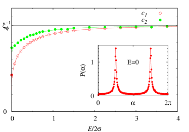
Figure 1: A lack of phase randomization leads to a distinctive band center anomaly in the conductance $g_{n}$ through a disordered wire (1) of length $n=12000$ with next-neighbor correlations (17) of the potential and $\sigma=1/150$ (RPR localization length $\xi_{\phi}=2/\sigma=300$). The main panel shows the mean logarithm $c_{1}=-(1/2n)\langle\ln g_{n}\rangle$ and its variance $c_{2}=(1/4n)\operatorname{Var}\ln g_{n}$ from numerical simulations (data points) and the analytical expressions (21,24a) (solid lines), scaled to $\xi_{\phi}^{-1}$. The inset shows the distribution of the reflection phase $P(\alpha)$ at the band center, calculated numerically as well as analytically (18).

We consider the one-dimensional Anderson model

$$-\Psi_{n+1}-\Psi_{n-1}+U_{n}\Psi_{n}=E\,\Psi_{n}$$ (1)

with a weak disordered potential $U_{n}$, $\langle U_{n}\rangle=0$ with $|U_{n}|\ll 1$.

The correlation function $\langle U_{n}U_{m}\rangle=\sigma(n,m)$ is assumed to be invariant under a finite translational shift $\sigma(n+Q,m+Q)=\sigma(n,m)$. The minimal period $Q$ does not need to be identical with the lattice constant. This accommodates the cases of structural and chemical disorder, or carefully engineered disorder, e.g., with masks. For $Q=1$ the correlation function is generally written as

$$\langle U_{n}U_{n^{\prime}}\rangle=\sigma_{n-n^{\prime}},\qquad\sigma_{n}=\sigma_{-n}.$$ (2)

The localization length $\xi$ is accessible via the dimensionless conductance (transmission probability) $g_{n}$ of the system of length $n$, $\xi^{-1}=-\lim_{n\to\infty}(1/2n)\langle\ln g_{n}\rangle$. In order to quantify deviations from universality we consider the complete statistics of the conductance fluctuations obtained from the generating function

$$\chi(\mu)=\lim_{n\to\infty}\frac{1}{n}\ln\langle g_{n}^{-\mu/2}\rangle=\sum\limits_{s=1}^{\infty}\frac{c_{s}\mu^{s}}{s!},\quad\mu\geq 0.$$ (3)

The localization length is given by $\xi=c_{1}^{-1}$. In single-parameter scaling ATAF , $c_{2}=c_{1}$, and $c_{s}=0$ for $s\geq 3$, corresponding to a log-normal distribution of $g_{n}$. In this paper we concentrate on the first two coefficients $c_{1}$ and $c_{2}$. We base our analysis on the exact phase formalism Halperin ; LGP , which we extend to the case of correlated disorder.

For the sake of definiteness assume the wave is reflected from the right end of a system of length $n\gg\xi$, with reflection amplitude $r_{n}=\sqrt{1-g_{n}}\exp(i\alpha_{n})$. The reflection phase $\alpha_{n}\in(0,2\pi)$ is related to the wave function by

$$\frac{\Psi_{n}}{\Psi_{n-1}}=\frac{1+e^{i\alpha_{n}}}{e^{ik}+e^{-ik+i\alpha_{n}}},\quad E=-2\cos k,$$ (4)

while the conductance $g_{n}$ is obtained from

$$\lambda_{n}\equiv-\frac{1}{2}\ln g_{n}=\frac{1}{2}\ln|\Psi_{n}^{2}+\Psi_{n-1}^{2}+E\,\Psi_{n}\Psi_{n-1}|.$$ (5)

Up to the second order in disorder strength, the statistical evolution of the phase and conductance with increasing system size is described by the recursion relations

$$\alpha_{n+1}-\alpha_{n} = 2k-2K_{n}(\alpha_{n}),$$ (6a)

$$\lambda_{n+1}-\lambda_{n} = K^{\prime}_{n}(\alpha_{n})+\big{(}K^{\prime}_{n}(\alpha_{n})\big{)}^{2},$$ (6b)

where the prime stands for the derivative with respect to $\alpha_{n}$ and the function $K_{n}(\alpha)$ is given by

$$K_{n}(\alpha)=\frac{\Phi_{n}(\alpha)}{1+\Phi^{\prime}_{n}(\alpha)},\quad\Phi_{n}(\alpha)=\frac{U_{n}}{v}(1+\cos\alpha),$$ (7)

with the group velocity $v=|\partial E/\partial k|$.

There exsist two major obstacles in the derivation of the Fokker-Planck equation for the joint probability density $P_{n}(\alpha,\lambda)$ from Eqs. (6a,6b). First, the wave-number $k$ on the right-hand side of Eq. (6a) is not small. Second, the values of $K_{n}$ are correlated at different sites. These difficulties can be circumvented by monitoring the variables $\alpha_{n}$ and $\lambda_{n}$ with a step of $q$ sites Lambert . We parameterize the energy $E=-2\cos\pi p/q+\varepsilon$ with small $\varepsilon\ll 1$ and integer $p$, and choose $q$ to be much larger than the correlation radius of the potential. Thus, the change of the phase over $q$ sites $\delta\alpha=\alpha_{n+q}-\alpha_{n}$ is small,

$$\delta\alpha_{n}=\frac{2\varepsilon q}{v}-2\sum\limits_{s=0}^{q-1}\Phi_{n+s}(\alpha+2ks)$$ (8)

$$\quad+2\sum\limits_{s=0}^{q-1}\sum\limits_{m=s}^{q-1}\frac{2}{1+\delta_{ms}}\Phi_{n+s}(\alpha+2ks)\Phi^{\prime}_{n+m}(\alpha+2km),$$

to the second order in the potential. Similarly, the increment $\delta\lambda=\lambda_{n+q}-\lambda_{n}$ is given by

$$\delta\lambda_{n}=\sum\limits_{s=0}^{q-1}\Phi^{\prime}_{n+s}(\alpha+2ks)$$ (9)

$$\quad-\sum\limits_{s=0}^{q-1}\sum\limits_{m=s}^{q-1}\frac{2}{1+\delta_{ms}}\Phi_{n+s}(\alpha+2ks)\Phi^{\prime\prime}_{n+m}(\alpha+2km).$$

In the limit o weak disorder the recurrent relations Eqs. (9,8) lead to the Fokker-Planck equation for the joint probability density $P_{n}(\alpha,\lambda)$

$$\frac{\partial P_{n}}{\partial n}=-\frac{\partial}{\partial\alpha}F(\alpha)P_{n}+\frac{1}{2}\frac{\partial^{2}}{\partial\alpha^{2}}D(\alpha)P_{n}$$ (10)

$$-\frac{\partial}{\partial\lambda}F_{1}(\alpha)P_{n}+\frac{1}{2}\frac{\partial^{2}}{\partial\lambda^{2}}D_{1}(\alpha)P_{n}+\frac{\partial}{\partial\lambda}\frac{\partial}{\partial\alpha}D_{01}(\alpha)P_{n}.$$

The drift and diffusion coefficients, which determine the phase distribution $P_{n}(\alpha)$, are

$$F(\alpha)=\frac{1}{q}\langle\delta\alpha_{n}\rangle,\ \ D(\alpha)=\frac{1}{q}\sum\limits_{m=-\infty}^{\infty}\!\!\langle\delta\alpha_{n}\delta\alpha_{n+mq}\rangle.$$ (11)

In the case of the correlated disoder (2) with $Q=1$, these coefficients are related by $F=2\varepsilon/v+(1/4)\partial D/\partial\alpha$. The other coefficients in Eq. (10) are given by

$$F_{1}(\alpha)=\frac{1}{q}\langle\delta\lambda_{n}\rangle,\ \ D_{1}(\alpha)=\frac{1}{q}\sum\limits_{m=-\infty}^{\infty}\!\!\langle\delta\lambda_{n}\delta\lambda_{n+mq}\rangle.$$

$$D_{01}(\alpha)=\frac{1}{q}\sum\limits_{m=-\infty}^{\infty}\!\!\langle\delta\alpha_{n}\delta\lambda_{n+mq}\rangle.$$ (12)

Thus, we have derived Fokker-Planck equations (10), which describe the system in the vicinity of a given rational energy $E=-2\cos\pi p/q$ with $q\geq 2$. The potential fluctuations are assumed to be restricted within the conduction band, so that $|E\pm U_{n}|<2$. In particular Eq. (10) does not apply in the vicinity of the band edge, where any fluctuation is strong. The latter case has to be treated separately. The effect of dichotomic correlated disorder near the band edge was studied in Ref. DEL2003b .

The equation for the phase distribution function $P_{n}(\alpha)$ is readily obtained by integrating Eq. (10) over the variable $\lambda$. There exists, however, no general way to derive a similar equation for the distribution $P_{n}(\lambda)$. The calculation of the generating function $\chi(\mu)$ hence requires the analysis of the full density $P_{n}(\alpha,\lambda)$. Such analysis is greatly simplified for RPR, which implies the factorization $P_{n}(\alpha,\lambda)=(2\pi)^{-1}P_{n}(\lambda)$. In this case a closed equation for $P_{n}(\lambda)$ can be derived by averaging Eq. (10) over the phase

$$\frac{\partial P_{n}(\lambda)}{\partial n} = \frac{1}{\xi_{\phi}}\frac{\partial P_{n}(\lambda)}{\partial\lambda}+\frac{1}{2\xi_{\phi}}\frac{\partial^{2}P_{n}(\lambda)}{\partial\lambda^{2}},$$ (13a)

$$\frac{1}{\xi_{\phi}} = \int_{0}^{2\pi}\frac{d\alpha}{2\pi}F_{1}(\alpha)=\int_{0}^{2\pi}\frac{d\alpha}{2\pi}D_{1}(\alpha),$$ (13b)

where $\xi_{\phi}$ is the localization length in the presence of RPR. The last equality in Eq. (13b) follows directly from Eq. (6b), which implies that the first and second moment of the increment of $\lambda$ are equal if the phase is randomized. The generating function (3) calculated from Eq. (13b) has the parabolic shape $\chi(\mu)=\mu(1+\mu/2)/\xi_{\phi}$. Hence, RPR implies single-parameter scaling in the localized regime, even in the presence of correlated disorder [this statement holds also for hopping disorder, which modifies the expression for $K_{n}$, while Eqs. (6a,6b) retain their form.]

It is instructive to calculate $\xi_{\phi}$ for correlations of the type (2). Taking the integrals in Eq. (13b) we reproduce the result of Ref. IK

$$\frac{1}{\xi_{\phi}}=\frac{1}{2v^{2}}\sum\limits_{s=-\infty}^{\infty}\sigma_{s}e^{2iks}.$$ (14)

It is important to remember, however, that $\xi_{\phi}=\xi$ only if RPR holds. This brings us to the question: What are the conditions for RPR, and what are the implications for the localized wave functions when RPR does not occur?

As a first example to illustrate the effect of short-range correlations on the reflection phase statistics, we consider disorder of the type (2) with next-neighbor correlations only, $\sigma_{s\geq 3}=0$. We let $q=2p,q\gg 1$ and obtain from Eq. (11)

$$D(\alpha)=2\sigma_{0}-(\sigma_{0}-2\sigma_{1})\sin^{2}\alpha.$$ (15)

The Fokker-Planck equation for the stationary phase distribution $P(\alpha)$ is simplified to

$$-\varepsilon\frac{\partial}{\partial\alpha}P+\frac{1}{2}\frac{\partial}{\partial\alpha}\sqrt{D}\frac{\partial}{\partial\alpha}\sqrt{D}P=0.$$ (16)

Its solution at the band center $\varepsilon=E=0$ is given by $P\propto[D(\alpha)]^{-1/2}$. Note, that the solution slightly deviates from the constant even for the white-noise potential ($\sigma_{1}=0$), which is the source of the so-called Kappus-Wegner anomaly KW ; Derrida ; ST2003a . The next-neighbor statistical correlations can induce far stronger deviations from RPR. Indeed, for $\sigma=\sigma_{1}=-\sigma_{0}/2$,

$$\langle U_{n}U_{n^{\prime}}\rangle=2\sigma\delta_{nn^{\prime}}-\sigma\delta_{nn^{\prime}\pm 1},$$ (17)

the solution to Eq. (16) is singular at $\varepsilon=0$, because the function $D(\alpha)$ develops a zero for $\alpha=\pm\pi/2$.

At the level of Eq. (16) the situation is analogous to the band center Dyson singularity Dyson in the presence of hopping disorder. Hence, the correlations turned a weak anomaly into a strong anomaly. While the usual Dyson singularity appears as a consequence of an exact “chiral” symmetry of the wire, such symmetry is limited to the first two orders in disorder strength for the correlated disorder (17). Using the decomposition $U_{n}=u_{n}-u_{n-1}$ with $\langle u_{n}u_{n^{\prime}}\rangle=\sigma\delta_{nn^{\prime}}$, and taking also the fourth order terms $\langle u_{n}^{4}\rangle=\eta^{2}$ in the potential into account, we derive at the band center the regularized phase distribution

$$P_{E=0}(\alpha)\propto\left(\cos^{2}\alpha+(\eta^{2}-\sigma^{2})/4\sigma\right)^{-1/2},$$ (18)

which becomes more singular for lower disorder strength. The probability density $P_{E=0}(\alpha)$ acquires a non-universal dependence on the shape of the distribution function of the potential via the relation between its fourth and second moment. Slightly away from the band center, $\varepsilon\gg\sqrt{\sigma(\eta^{2}-\sigma^{2})}$, the fourth-order terms play no role and the phase distribution is described by the solution of Eq. (16) with $D=4\sigma\cos^{2}\alpha$,

$$P(\alpha)\propto\int_{0}^{\infty}\!\!dy\,\frac{e^{-\varepsilon y/2\sigma}}{\sqrt{y^{2}\cos^{2}\alpha+y\sin 2\alpha+1}}.$$ (19)

The lack of RPR is necessarily reflected in an anomaly of the density of states, due to the node-counting theorem Schmidt ; Buettiker1993 ; this also implies a different statistics of time delays $\tau=\partial\alpha/\partial E$, for which the increments are obtained by differentiating Eq. (8) with respect to $\varepsilon$.

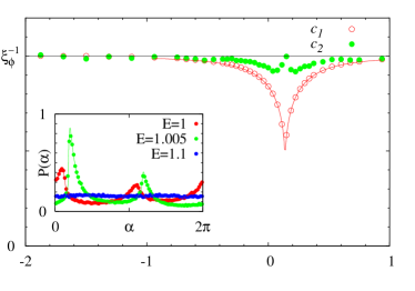
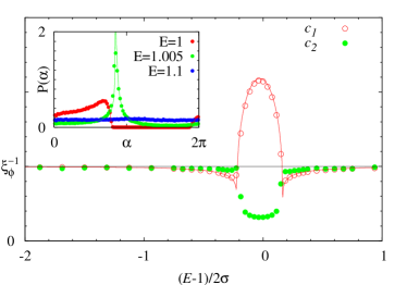
Figure 2: The mean logarithm of the conductance and its variance are calculated numerically for the system (1) of the large length $n$. The coefficients $c_{1}=-(1/2n)\langle\ln g_{n}\rangle$ and $c_{2}=(1/4n)\operatorname{Var}\ln g_{n}$ are plotted as the function of energy near the quarter band $E=1$. The disorder is generated by $U_{n}=2u_{n}-u_{n+1}-u_{n-1}$ (top panel) and $U_{n}=2u_{n+1}-u_{n}-u_{n-1}$ (bottom panel), where the random numbers $u_{n}=0$ unless $n$ is a multiple of $3$ and $\langle u_{3m}u_{3m^{\prime}}\rangle=\sigma\delta_{mm^{\prime}}$, $\sigma=1/150$. The insets show the distribution function of the reflection phase. The solid lines are obtained from the solution of Eq. (10) with $p=-1,q=3$. The RPR localization length $\xi_{\phi}$ is obtained from Eq. (13b).

We now explore the implications for the transmission properties of the system. For the specific correlations (17), the Fokker-Planck equation (10) simplifies near $E=0$ by

$$\frac{\partial P_{n}}{\partial n}=-\varepsilon\frac{\partial P_{n}}{\partial\alpha}+2\sigma\left[\frac{\partial}{\partial\alpha}\cos\alpha+\frac{1}{2}\sin\alpha\frac{\partial}{\partial\lambda}\right]^{2}P_{n}.$$ (20)

The coefficient $c_{1}$ is obtained directly by averaging the expression (9) with the stationary phase distribution (19). The result is

$$c_{1}=\sigma\int_{0}^{2\pi}\!\!\!d\alpha\,P(\alpha)\,\cos^{2}\alpha=-\frac{\varepsilon}{2}\,{\rm Im}\,\frac{K_{1}(i\varepsilon/2\sigma)}{K_{0}(i\varepsilon/2\sigma)},$$ (21)

where $K_{\nu}(x)$ is the modified Bessel function. The singularity in Eq. (21) in the limit $\varepsilon\to 0$ is again regularized in the fourth order of the potential. In the weak disorder limit we find at the band center $\xi/\xi_{\phi}=\ln 8\sqrt{\sigma/(\eta^{2}-\sigma^{2})}$.

From Eq. (20) we can determine all coefficients $c_{s}$ recursively ST2003b ; ST2003a ; ST2003c . A double Laplace transform

$$\tilde{P}_{\chi}(\alpha,\mu)=\sum\limits_{n}\int_{-\infty}^{\infty}\!\!d\lambda\,e^{\lambda\mu-\chi(\mu)n}P_{n}(\alpha,\lambda),$$ (22)

reduces Eq. (20) to the eigenvalue problem

$$-\varepsilon\frac{\partial\tilde{P}_{\chi}}{\partial\alpha}+2\sigma\left[\frac{\partial}{\partial\alpha}\cos\alpha-\frac{\mu}{2}\sin\alpha\right]^{2}\tilde{P}_{\chi}=\chi(\mu)\tilde{P}_{\chi}.$$ (23)

The generating function $\chi(\mu)$ can be obtained perturbatively in $\mu$, taking the solution $P(\alpha)$ of Eq. (19) as zero approximation. In particular, the variance $c_{2}$ is given by

$$c_{2} = \sigma-c_{1}-\int_{0}^{2\pi}\!\!\!d\alpha\,(c_{1}-\sigma\cos^{2}\alpha)G(\alpha),$$ (24a)

$$G(\alpha) = {\cal L}_{\alpha}^{-1}\,(c_{1}\!-\!\sigma\cos^{2}\alpha\!+\!\sigma\frac{\partial}{\partial\alpha}\sin 2\alpha)P(\alpha),$$ (24b)

$${\cal L}_{\alpha} = -\frac{\varepsilon}{2\sigma}\frac{\partial}{\partial\alpha}+\frac{\partial}{\partial\alpha}\cos\alpha\frac{\partial}{\partial\alpha}\cos\alpha.$$ (24c)

In order to illustrate our predictions, we compare them in Fig. 1 to the results of numerical simulations. The numerical results agree with the theory, without any adjustable parameter. The main panel shows the energy dependence of $c_{1}$ and $c_{2}$ near the band center [Eqs. (21,24a)], which clearly deviates from the single-parameter scaling prediction $c_{1}=c_{2}=\xi_{\phi}^{-1}$. The inset shows the phase distribution (18) at the band center.

In general, RPR is completely violated if the diffusion coefficient $D(\alpha)$ has zeros as the function of $\alpha$. The reflected wave then mantains a strict phase relation with the incoming wave. For the correlated disorder of the type (2) such relation (phase selection) can only occur at the band center. The restriction is lifted for correlations with $Q\neq 1$. In Fig. (2) we provide examples of a quarter band anomaly, caused by a disorder correlations with $Q=3$. Following this recipe, strong anomalies can be produced in a vicinity of arbitrary rational values of the wave length $2q/p$ by a suitably correlated weak disorder potential with $Q=q$. This is in striking contrast to the case of white-noise disorder, which produces only a weak anomaly, and only at a single spectral point (the band center).

In conclusion we show that the 1D Anderson model with a weak short-range correlated potential may demonstrate strong anomalies near specific spectral points. Such anomalies can be used to strongly modify the transmission properties of electronic wires and photonic wave guides in very small energy windows provided the phase coherence preserved over a long distance. In these windows the reflected wave develops a preferred phase relation with the incoming wave. These properties indicate that disorder correlations may be favorably employed in the design of photonic or electronic filters.

We gratefully acknowledge discussions with Piet Brouwer and the warm hospitality in the Lorentz Institute in Leiden, where part of this work was done.

References

- (1) A. Ishimaru, Wave Propagation and Scattering in Random Media (Academic, New York, 1978).
- (2) P. Sheng, Scattering and Localization of Classical Waves in Random Media (World Scientific, Singapore, 1990).
- (3) R. Berkovits and S. Feng, Phys. Rep. 238, 135 (1994).
- (4) P. Sebbah, O. Legrand, B. A. van Tiggelen, and A. Z. Genack, Phys. Rev. E 56, 3619 (1997).
- (5) P. W. Anderson, D. J. Thouless, E. Abrahams, and D. S. Fisher, Phys. Rev. B 22, 3519 (1980).
- (6) O. N. Dorokhov, Pis’ma Zh. Eksp. Teor. Fiz. 36, 259 (1982) [JETP Letters 36, 318 (1982)].
- (7) P. A. Mello, P. Pereyra, and N. Kumar, Ann. Phys. (NY) 181, 290 (1998).
- (8) K. B. Efetov, Adv. Phys. 32, 53 (1983).
- (9) C. W. J. Beenakker, Rev. Mod. Phys. 69, 731 (1997).
- (10) F. J. Dyson, Phys. Rev. 92, 1331 (1953).
- (11) P. W. Brouwer, C Mudry, A. Furusaki, Phys. Rev. Lett. 84, 2913 (2000)
- (12) S. Ryu, C. Mudry, and A. Furusaki, Phys. Rev. B 70, 195329 (2004).
- (13) H. Schomerus and M. Titov, Eur. Phys. J. B 35, 421 (2003).
- (14) H. Schomerus and M. Titov, Phys. Rev. B 67, 100201(R) (2003).
- (15) L. I. Deych, M. V. Erementchouk, A. A. Lisyansky, Phys. Rev. Lett 90, 126601 (2003).
- (16) M. Titov and H. Schomerus, Phys. Rev. Lett. 91, 176601 (2003).
- (17) M. Kappus and F. Wegner, Z. Phys. B: Condens. Matter 45, 15 (1981).
- (18) B. Derrida and E. Gardner, J. Phys. (Paris) 45, 1283 (1984).
- (19) M. J. de Oliveira, A. Petri, Phys. Rev. B 56, 251 (1997).
- (20) L. I. Deych, M. V. Erementchouk, A. A. Lisyansky, Physica B 338, 79 (2003).
- (21) F. M. Izrailev and A. A. Krokhin, Phys. Rev. Lett. 82, 4062 (1999).
- (22) B. I. Halperin, Phys. Rev. 139, A104 (1965).
- (23) I. M. Lifshitz, S. A. Gredeskul, and L. A. Pastur, Introduction to the Theory of Disordered Systems (Wiley, New York, 1988).
- (24) C. J. Lambert, Phys. Rev. B 29, R1091 (1984).
- (25) L. I. Deych, M. V. Erementchouk, and A. A. Lisyansky, Phys. Rev. B 67, 024205 (2003).
- (26) H. Schmidt, Phys. Rev. 105, 425 (1957).
- (27) M. Büttiker, J. Phys.: Condens. Matter 5, 9361 (1993).