Monte Carlo algorithms for charged lattice gases

Abstract

We consider Monte Carlo algorithms for the simulation of charged lattice gases with purely local dynamics. We study the mobility of particles as a function of temperature and show that the poor mobility of particles at low temperatures is due to “trails” or “strings” left behind after particle motion. We introduce modified updates which substantially improve the efficiency of the algorithm in this regime.

I Introduction

The properties of many condensed matter systems can not be understood without considering the Coulombic interaction. DNA, proteins, polyelectrolytes, colloids and even water are all structured by electrostatics, which must be reproduced faithfully in any numerical study. Unfortunately, the simulation of the electrostatic interactions is difficult; due to the slow decay of the potential in $1/r$ one can not truncate the interaction Frenkel and Smit (2002) as is often done with other molecular interactions. Most working codes now use a variant of the Ewald sum to account for the interaction between periodic images of the basic simulation cell. As a consequence the time need to evaluate the electrostatic interaction can dominate in the simulation of charged systems.

In a Monte Carlo simulation with the Ewald method, the motion of a single charge requires summing its interactions with the $N-1$ other charges and their periodic images, resulting in a $\mathcal{O}\bigl{(}N^{2}\bigr{)}$ computational cost per sweep. This becomes impractical when $N$ is large. In simulations with explicit modeling of all charges $N>10^{4}$ is commonly required. In molecular dynamics the situation is better: when all particles are moved simultaneously, better CPU time scalings are possible ranging from $\mathcal{O}\bigl{(}N\bigr{)}$ for multigrid algorithms Shan et al. (2005) to $\mathcal{O}\bigl{(}N^{3/2}\bigr{)}$ for an optimized Ewald summation Perram et al. (1988). However these molecular dynamics codes are complex to implement.

The unfavorable complexity of conventional Monte Carlo methods originates in the use of the electrostatic potential $\Phi$, which is the solution to Poisson’s equation

$$\nabla^{2}\Phi=-\rho/\epsilon.$$

This equation has a unique solution for given charge distribution and boundary conditions. When a charge is moved, the new solution for $\Phi$ is computed and the interaction energy $q_{i}\Phi(\mathbf{r}_{i})$ of the moved charge with all other charges $q_{i}$ in the system changes. The electrostatic interaction implemented in this way is instantaneous. Note however Maggs and Rossetto (2002), the thermodynamical study of charged systems does not require instantaneous Coulombic interactions: The free energy is also correctly sampled when only Gauss’s law

$$\mathrm{div}\,\mathbf{E}=\rho/\epsilon$$

is imposed on the electric field. The fact that solutions to Gauss’s law are not unique results in an extra flexibility which allows one to implement a purely local Monte Carlo scheme for the simulation of systems with electrostatic interactions. The computation effort is reduced to $\mathcal{O}\bigl{(}N\bigr{)}$ per Monte Carlo sweep. The disadvantage of the algorithm is that it requires a grid to discretize the electrostatic degrees of freedom, however this is also true of multigrid and Fourier methods used for molecular dynamics.

The final efficiency of the Monte Carlo algorithm depends on the number of sweeps required to sample independent configurations which in turn is a function of the particle mobility resulting from the Monte Carlo dynamics. Highly mobile charges enable one to generate independent configurations rapidly; if charges were to become “trapped” or “localized” due to their interaction with the field it could prevent the generation of uncorrelated samples. Monitoring the acceptance rate of particle updates may only give partial information in that on the total efficiency of an algorithm. For instance trapped particles could move locally (resulting in a good acceptance rate) without being able to explore all of space.

In this article we perform a detailed study of the charge mobility $\mu$ in local Monte Carlo algorithms in order to compare efficiencies of various implementations. Firstly we develop a technique to measure $\mu$ by relating the mobility to the dynamics of the average electric field, $\bar{\mathbf{E}}$. The mobility will be studied as a function of temperature. With our previous implementation, $\mu$ drops dramatically at low temperatures, becoming unmeasurable for parameters which are needed to study typical materials: For instance monovalent ions in water at room temperature where $\epsilon=78$, $T=300~{}\text{K}$, $a=1~{}\text{\r{A}}$ with $a$ the mesh size. The drop in efficiency originates in the constrained dynamics of the electric field, leading to the generation of “trails” or “strings” which trap particles at low temperature and suppress their mobility.

We will explore ways of reducing this trapping. The update law introduced previously Maggs and Rossetto (2002) for particle motion is not the only way one can move a charge. Even if each charge update must be accompanied by some field update, the latter is only loosely constrained. Duncan, Sedgewick, and Coalson recently used this fact to introduce Duncan et al. (2005) a better particle-plaquette update. We will present several field updating schemes leading to less trapping. These schemes are very flexible in that they have a freely adjustable “spreading” parameter $w$, upon which their effects and their computational complexity depend. Schemes which use a larger spreading parameter are more time-consuming but lead to much larger efficiencies at physically interesting temperatures.

We have already shown Rottler and Maggs (2004) that off-lattice implementations of the algorithm (using continuous interpolation of charges with splines) do not suffer the mobility drop that we discuss in this paper. Rather, our present work is motivated by the existence of a wide spectrum of interesting and useful lattice models. For example, it is known Panagiotopoulos and Kumar (1999); Panagiotopoulos (2000); Moghaddam and Panagiotopoulos (2003) that finely discretized lattice fluids exhibit the same critical behavior as continuum fluids. Another example is the bond fluctuation model for polymers Carmesin and Kremer (1988); Binder and Paul (1997) which is rather easily generalized to study charged polymers, or polyelectrolytes. All these models already use “spread” or extended particles where the hard cores of the particles span several lattice sites in order to reduce lattice artefacts to an acceptable level.

We will begin (Sec. II) with a description of the theoretical basis and implementation of local Monte Carlo algorithms with electrostatics. In Sec. III we show how to measure the mobility of charges and apply the method to the simplest algorithm. We interpret the behavior of the acceptance rate and mobility as a function of temperature (Sec. IV), introducing the concept of field trails or strings. We show how to increase particle mobility in Secs. V, VI. Finally we will present the CPU time for representative simulations and give the reader an estimate of optimal parameters.

II Monte Carlo algorithm

We give a basic description of the algorithm previously developed in Refs. Maggs and Rossetto (2002); Maggs (2002, 2004). We first recall its theoretical basis, and then present the simplest implementation, highlighting places where the method can be further optimized for speed.

II.1 Theoretical foundation

In order to sample configurations of a system containing charges, we require that a set $\{\mathbf{r}_{i}\}$ of particle positions is generated with weight

$$z\bigl{(}\{\mathbf{r}_{i}\}\bigr{)}=e^{-\beta\left[{\textstyle\frac{1}{2}\int_{V}}\rho(\mathbf{r};\{\mathbf{r}_{i}\})\Phi(\mathbf{r};\{\mathbf{r}_{i}\})\>\mathrm{d}{{}^{3}}r\;+\;\mathcal{U}(\{\mathbf{r}_{i}\})\right]}$$

where $\rho\bigl{(}\mathbf{r};\{\mathbf{r}_{i}\}\bigr{)}=\sum_{i}q_{i}\delta\bigl{(}\mathbf{r}-\mathbf{r}_{i}\bigr{)}$ is the charge distribution of the configuration, $\Phi\bigl{(}\mathbf{r};\{\mathbf{r}_{i}\}\bigr{)}$ is the unique solution to Poisson’s equation, and $\mathcal{U}\bigl{(}\{\mathbf{r}_{i}\}\bigr{)}$ is the potential of all other interactions. The partition function then is

$$\mathcal{Z}=\int\Bigl{(}\prod\limits_{i}\>\mathrm{d}{{}^{3}}r_{i}\Bigr{)}z\bigl{(}\{\mathbf{r}_{i}\}\bigr{)}.$$

In the usual treatment of electrostatic interactions the electric field is given by $\mathbf{E}_{P}=-\mathrm{grad}\,\Phi$: it is unique and satisfies both Gauss’s law $\mathrm{div}\,\mathbf{E}_{P}=\rho/\epsilon$ and the static version of Faraday’s law $\mathrm{curl}\,\mathbf{E}_{P}=\mathbf{0}$. We chose the convention where the potential of a charge $q$ is $q/4\pi\epsilon r$. The algorithm is based on relaxing Faraday’s law so that $\mathbf{E}=\mathbf{E}_{P}+\mathrm{curl}\,\mathbf{Q}$, a decomposition familiar from the Coulomb gauge of electrodynamics. Fourier transforming we find that $\mathbf{E}_{P}$ is longitudinal:

$$(\mathbf{E}_{P})_{\mathbf{k}}=-i\mathbf{k}\Phi_{\mathbf{k}}\parallel\mathbf{k}$$

and that $\mathrm{curl}\,\mathbf{Q}$ is transverse:

$$(\mathrm{curl}\,\mathbf{Q})_{\mathbf{k}}=i\mathbf{k}\negmedspace\times\negmedspace\mathbf{Q}_{\mathbf{k}}\perp\mathbf{k}.$$

As a consequence, the electrostatic energy

$$\begin{split}\frac{\epsilon}{2}\int_{V}\mathbf{E}^{2}\>\mathrm{d}{{}^{3}}r&=\frac{\epsilon}{2}\left(\int_{V}{\mathbf{E}_{P}}^{2}\>\mathrm{d}{{}^{3}}r+\int_{V}(\mathrm{curl}\,\mathbf{Q})^{2}\>\mathrm{d}{{}^{3}}r\right)\\ &=\frac{1}{2}\int_{V}\rho\Phi\>\mathrm{d}{{}^{3}}r+\frac{\epsilon}{2}\int_{V}(\mathrm{curl}\,\mathbf{Q})^{2}\>\mathrm{d}{{}^{3}}r\end{split}$$

so that the statistical weight of a configuration of charges and field is

$$\begin{split}z^{\prime}\bigl{(}\{\mathbf{r}_{i}\},\mathbf{E}_{\perp}\bigr{)}&=e^{-\beta\left[\mathcal{U}(\{\mathbf{r}_{i}\})+{\textstyle\frac{\epsilon}{2}\int_{V}}\mathbf{E}^{2}\>\mathrm{d}{{}^{3}}r\right]}\\ &=z\bigl{(}\{\mathbf{r}_{i}\}\bigr{)}e^{-\beta{\textstyle\frac{\epsilon}{2}\int_{V}}\mathbf{E}_{\perp}^{2}\>\mathrm{d}{{}^{3}}r}\end{split}$$

where for clarity we have introduced the transverse field $\mathbf{E}_{\perp}=\mathrm{curl}\,\mathbf{Q}$. This field is constrained by $\mathrm{div}\,\mathbf{E}_{\perp}=0$; it is independent of the charge configuration. Thus, the partition function of the system of charges and field splits into two parts:

$$\begin{split}\mathcal{Z}^{\prime}&=\int\Bigl{(}\prod\limits_{i}\>\mathrm{d}{{}^{3}}r_{i}\Bigr{)}\mathcal{D}\mathbf{E}_{\perp}\delta\bigl{(}\mathrm{div}\,\mathbf{E}_{\perp}\bigr{)}z^{\prime}\bigl{(}\{\mathbf{r}_{i}\},\mathbf{E}_{\perp}\bigr{)}\\ &=\left(\int\Bigl{(}\prod\limits_{i}\>\mathrm{d}{{}^{3}}r_{i}\Bigr{)}z\bigl{(}\{\mathbf{r}_{i}\}\bigr{)}\right)\\ &\quad\times\left(\int\mathcal{D}\mathbf{E}_{\perp}\delta\bigl{(}\mathrm{div}\,\mathbf{E}_{\perp}\bigr{)}e^{-\beta{\textstyle\frac{\epsilon}{2}\int_{V}}\mathbf{E}_{\perp}^{2}\>\mathrm{d}{{}^{3}}r}\right)\\ &=\mathcal{Z}\times\mathcal{Z}_{\text{tr}}\end{split}$$ (1)

where $\mathcal{Z}_{\text{tr}}$ is the partition function of transverse field. The statistical weight of a configuration of charges is $z\bigl{(}\{\mathbf{r}_{i}\}\bigr{)}\times\mathcal{Z}_{\text{tr}}$; all the weights have been multiplied by the same constant. Hence configurational probabilities are left unchanged. Of course sampling this system requires introducing Monte Carlo moves appropriate for integrating over $\mathbf{E}_{\perp}$ degrees of freedom.

II.2 A charged lattice gas

We consider a cubic simulation cell of $L^{3}$ sites with periodic boundary conditions. Particles are placed on sites of a lattice with mesh spacing $a$, and field variables representing electric flux are defined on links. The electric field divergence at a site is the sum of fluxes over the six outgoing links. (See Fig. 1.) Transverse field degrees of freedom appear as a nonzero line integral of $\mathbf{E}$ on plaquettes of the lattice.

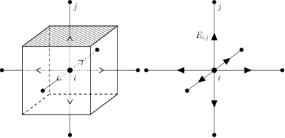
Figure 1: Left: cubic lattice mesh around site $i$. The electric flux $\phi_{i,j}$ flowing upward through the hashed cube face is assigned to link $(i,j)$ on the right: $E_{i,j}=\phi_{i,j}/a^{2}$. Field divergence at $i$ equals the outward flux through the cube surface, $\sum_{j\in\{\text{NN}\}}E_{i,j}$ where NN stands for nearest neighbors. In following figures only two dimensions of the lattice will be shown for clarity.

To start a simulation we must construct a state consistent with Gauss’s law. We initialize the electric field for the simulation with a single sweep through the network: We use a procedure that follows a Hamiltonian path through the lattice. Such a path visits each site just once and traverses each link either once or zero times. We begin by initializing all field values on the lattice to zero and start at an arbitrary point $1$ of the lattice; the node $1$ holds the charge $q_{1}$. A single link of the path, $\{1,2\}$, connects it to site $2$, on which we set the outgoing field to $q_{1}/a^{2}\epsilon$; Gauss’s law is now fulfilled on site $1$ and we move to the node $2$.

At each step, on arriving at site $i$ holding $q_{i}$, we have already solved the Gauss constraint for sites $\{1,\ldots,i-1\}$. The incoming link to the site, $\{i-1,i\}$, thus bears the initialized field $E_{i-1,i}=\left(\sum_{j=1}^{j=i-1}q_{j}\right)/a^{2}\epsilon$. We now set the outgoing field $E_{i,i+1}$ to $\left(\sum_{j=1}^{j=i}q_{j}\right)/a^{2}\epsilon$ so that $E_{i,i-1}+E_{i,i+1}=q_{i}/a^{2}\epsilon$: Gauss’s law is now fulfilled on site $i$ and we go to site $i+1$. At the end of the path, we reach site $V=L^{3}$ with $E_{V-1,V}=\left(\sum_{j=1}^{j=V-1}q_{j}\right)/a^{2}\epsilon$. The imposition of periodic boundary conditions in charged systems is only possible if the total charge $Q$ is zero (otherwise the total energy is divergent). Thus $E_{V-1,V}=(Q-q_{V})/a^{2}\epsilon=-q_{V}/a^{2}\epsilon$ and Gauss’s law is satisfied everywhere on the lattice.

We take advantage of the new field degrees of freedom to construct local updates for charge moves. Consider an initial configuration $\rho^{(\text{i})}$ where a charge $q$ is at point $A$, and the initial electric field $\mathbf{E}^{(\text{i})}$ satisfies Gauss’s law ($\mathrm{div}\,\mathbf{E}^{(\text{i})}=\rho^{(\text{i})}/\epsilon$). If a trial places $q$ at point $B$, the final configuration is $\rho^{(\text{f})}=\rho^{(\text{i})}-q\delta\bigl{(}\mathbf{r}-\mathbf{r}_{A}\bigr{)}+q\delta\bigl{(}\mathbf{r}-\mathbf{r}_{B}\bigr{)}$, and a new solution for the field must be found. In order to remain consistent with Gauss’s law it is sufficient to add to $\mathbf{E}^{(\text{i})}$ field lines $\delta\mathbf{E}$ flowing from $B$ to $A$ and totalizing $q/\epsilon$ flux. The final field $\mathbf{E}^{(\text{f})}=\mathbf{E}^{(\text{i})}+\delta\mathbf{E}$ now satisfies again Gauss’s law for the final charge configuration:

$$\mathrm{div}\,\mathbf{E}^{(\text{f})}=\frac{\rho^{(\text{i})}}{\epsilon}+\frac{q}{\epsilon}\delta\bigl{(}\mathbf{r}-\mathbf{r}_{B}\bigr{)}-\frac{q}{\epsilon}\delta\bigl{(}\mathbf{r}-\mathbf{r}_{A}\bigr{)}=\frac{\rho^{(\text{f})}}{\epsilon}.$$

We call $\delta\mathbf{E}$ “the slaved update”. Nothing having been required of it except the total flux, we can choose it to be localized in space, so that charge moves result in local updates of the simulated system. In addition $\delta\mathbf{E}$ should be symmetrically chosen so that detailed balance applies to the forward and reverse updates. Our previous choice of $\delta\mathbf{E}$, which modifies just the link connecting $A$ to $B$ is illustrated in Fig. 2. Nevertheless, the “total flux” constraint lets us free to use more complex slaved updates. We will show in this paper that splitting $\delta\mathbf{E}$ into several lines helps increase the algorithm efficiency.

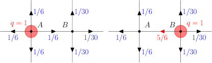
Figure 2: A pair of lattice sites, before and after a particle move. Left, the initial configuration is made up of a charge at $A$ and one solution to Gauss’s constraint: at $A$ the field divergence is six times $1/6$, equaling $q=1$ (in reduced units where $a=1$, $\epsilon=1$), and at $B$ it is $5\times 1/30-1/6=0$. Right, the charge has moved to $B$ and a flux $\delta E=q=1$ flowing from $B$ to $A$ has been added to the central link. Then Gauss’s law is again verified: at $A$, $\mathrm{div}\,\mathbf{E}=5\times 1/6-5/6=0$, and at $B$, $\mathrm{div}\,\mathbf{E}=5\times 1/30+5/6=1=q$.

Finally in order to correctly sample the partition function (1) we integrate over the transverse degrees of freedom of the electric field. We do this with Monte Carlo moves which change the circulation of the electric field, but do not modify its divergence. One way of doing this is by modifying the field on the four links defining a plaquette [Fig. 3(a)]. If one increases the field on links along the edge of a given plaquette by some constant value, at all sites $\mathrm{div}\,\mathbf{E}$ remains constant. This kind of update, being local, leads to diffusive dynamics for $\mathbf{E}_{\perp}$: $\mathcal{O}\bigl{(}L^{2}\bigr{)}$ sweeps are needed to yield an independent configuration.

An alternative method of integrating over $\mathbf{E}_{\perp}$ was introduced Levrel et al. (2005). These worm updates [Fig. 3(b)] make use of a biased random walk to generate a closed contour along which the field is modified. This contour visits typically $L^{3}$ sites and turns out to be particularly efficient at equilibrating the electric field at all length scales simultaneously: all Fourier modes of $\mathbf{E}_{\perp}$ decay at the same rate, $\mathcal{O}\bigl{(}1\bigr{)}$ sweeps are enough to produce an independent field configuration.

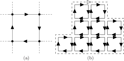
Figure 3: To update $\mathbf{E}_{\perp}$ one may choose between plaquette moves (a) which increase the field along a single plaquette edge, and worm moves [(b), dashed line] which modify it along the path of a given random walk. Both are thermodynamically equivalent since any field configuration reached through worm moves may be obtained through multiple plaquette updates [as shown in (b)] combined with updates of the $k=0$ mode of the field.

The aim of a Monte Carlo algorithm is to produce statistically independent configurations with minimum computational cost. The local updates described above allow one to efficiently update charge and field configurations. However in order to understand the global dynamics and convergence of the algorithm we shall study electric field autocorrelation functions. We now show that high mobility $\mu$ of the charges leads to fast decay of the field correlations.

III Measuring charge mobility

Under the dynamics of the algorithm, Figs. 2 and 3, $\mathbf{E}$ remains consistent with Gauss’s law at all times. Considering the time derivative of this law, we find

$$\mathrm{div}\,\frac{\partial\mathbf{E}}{\partial t}=\frac{\partial(\mathrm{div}\,\mathbf{E})}{\partial t}=\frac{1}{\epsilon}\frac{\partial\rho}{\partial t}$$

which translates in the implementation as

$$\mathrm{div}\,\delta\mathbf{E}=\frac{1}{\epsilon}\delta\rho.$$ (2)

Updates to the electric field can be considered as being due to local currents such that

$$\mathrm{div}\,\mathbf{J}+\frac{\delta\rho}{\delta t}=0,$$ (3)

where we introduced the time unit $\delta t=1$ Monte Carlo step. Combining Eqs. (2) and (3) we find

$$\mathrm{div}\,\delta\mathbf{E}=-\frac{\delta t}{\epsilon}\,\mathrm{div}\,\mathbf{J},$$

or

$$\delta\mathbf{E}=-\frac{\delta t}{\epsilon}\mathbf{J}+\delta t\,\mathrm{curl}\,\mathbf{H}$$ (4)

with $\mathbf{H}$ arbitrary. This is a discrete version of Ampere’s law of electromagnetism.

Spatially averaging Eq. (4), we find the change in the average electric field $\bar{\mathbf{E}}$ during an update,

$$\delta\bar{\mathbf{E}}=-\frac{\delta t}{\epsilon}\bar{\mathbf{J}}.$$ (5)

This equation is independent of $\mathbf{H}$; the last term in Eq. (4) gives zero due to periodic boundary conditions. This is consistent with the fact that local plaquette updates do not change the average electric field in a periodic system.

Our simulations are on a system containing $N$ mobile unit charges, either the symmetric plasma made up with $N/2$ particles of each sign ($q_{i}=\pm e$), or the one-component plasma (OCP) of $N$ positive charges moving in a fixed negative background. Linear response gives insight on the relation between charge mobility and field evolution. The electric current is due to the movement of mobile charges,

$$\mathbf{J}=\sum_{i}\mathbf{J}_{i}=\sum_{i}\rho_{i}\mathbf{v}_{i}=\sum_{i}q_{i}n_{i}\mathbf{v}_{i},$$ (6)

where $i\in\{+,-\}$, $\rho_{i}$ are charge densities and $n_{i}$ are number densities; $n_{-}=0$ for the OCP. On average, velocities are related to field by

$$\mathbf{v}_{i}=\mu q_{i}\mathbf{E}.$$ (7)

Given the charge symmetry of the algorithm, positive and negative ions in a symmetric plasma have the same mobility. Equations (6) and (7) lead to $\mathbf{J}=e^{2}(n_{+}+n_{-})\mu\mathbf{E}$. $n_{+}+n_{-}=n=N/V$ is the number density of mobile charges. Hence

$$\mathbf{J}=e^{2}n\mu\mathbf{E}.$$ (8)

We should bear in mind that these relations are phenomenological. For example, in Eq. (7) proportionality holds only when the field intensity is not too high. It will also become apparent that in certain limits $\mu$ can fall to zero for large, dilute systems.

Substituting Eq. (8) in Eq. (5), and replacing the difference equation by a differential equation we find that

$$\frac{\partial\bar{\mathbf{E}}}{\partial t}=-\frac{e^{2}n\mu}{\epsilon}\bar{\mathbf{E}}.$$ (9)

$\bar{\mathbf{E}}$ is the $\mathbf{k}=\mathbf{0}$ Fourier mode of the electric field. Equation (9) implies that the autocorrelation function of this mode behaves as follows:

$$\left\langle\bar{\mathbf{E}}(t^{\prime})\bar{\mathbf{E}}(t^{\prime}+t)\right\rangle_{t^{\prime}}=Ce^{-\tfrac{e^{2}n\mu}{\epsilon}t},$$

where $C$ is the squared amplitude of the thermal fluctuations of $\bar{\mathbf{E}}$. Measuring this autocorrelation function we find exponential decay with a characteristic time $\tau_{0}=\epsilon/(e^{2}n\mu)$ or equivalently a decay rate $\lambda_{0}=e^{2}n\mu/\epsilon$. We fit all our numerical data with a single exponential and verify the quality of the resulting curve by eye.

In our simulations we also monitored other modes of the field and found that the mode $\mathbf{k}=\mathbf{0}$ is the slowest. Higher modes of the field couple directly to plaquette updates as well as particle motion, and relax with the dispersion law $\lambda_{k}=\lambda_{0}+D_{E}k^{2}$ Maggs (2002). Larger $k$ are less sensitive to low particle mobility (low $\lambda_{0}$). They will not be considered further in this paper.

The time scale $\tau_{0}$ can be understood with a scaling argument. In order to produce two uncorrelated samples of the system, one should wait for the charges to diffuse through the characteristic correlation length of the system, the Debye length $l_{D}=\sqrt{\epsilon k_{B}T/e^{2}n}$. Thus $\tau_{0}={l_{D}}^{2}/D$, and $\lambda_{0}={\kappa_{D}}^{2}D=e^{2}nD/\epsilon k_{B}T$, with a diffusion constant $D$. We recover the above expression for the relaxation rate if we use the relation $D=k_{B}T\mu$. $D$ defined in this way relates to the mobility of charges under an external electric field (where opposite charges move opposite ways), not to the mobility under a constant external force (where all particles move together).

Thus we will measure the mobility of charges or, equivalently, their diffusion coefficient, by computing the autocorrelation function of the average electric field. This method has the additional advantage that we need not keep track of the winding of particles across the periodic cell boundaries.

IV Limiting factors for mobility

Acceptance rate is often used to monitor the efficiency of Monte Carlo simulations. However a high acceptance rate does not necessarily mean useful work has been performed. For example, the diffusion dynamics of point defects or interstitials in a crystal are very slow. In a Monte Carlo simulation most time is spent vibrating the atoms around their equilibrium positions; even in the limit of very rare diffusion events the acceptance rate of trial moves remains appreciable. Another example is magnetization reversal of an Ising ferromagnet. The state where all spins are oriented against an applied field is metastable but with very long lifetime; since the Metropolis algorithm is already very inefficient one uses rejection-free algorithms Novotny (1995) to update individual spins, unfortunately after a spin has been flipped it is almost certainly flipped back at the next step, so that the magnetization never reverses within accessible simulation times.

With our algorithm, a simulation performed at very low density, Fig. 4,

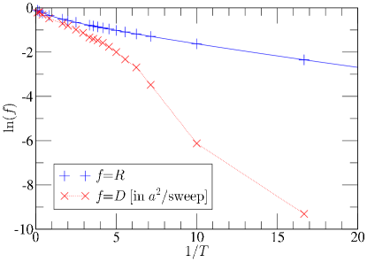
Figure 4: Logarithm of acceptance rate $R$, and of diffusion coefficient $D$ expressed in $a^{2}$ per particle sweep, versus inverse temperature. Solid line, Eq. 10; dotted line, guide to the eye. $R$ and $D$ are close to $1$ at high temperatures, but $D$ drops much faster than $R$ on decreasing $T$. One component plasma of two positive unit charges, box of size $L=15$.

shows that the diffusion coefficient $D$ of charges drops much faster at low temperatures than the acceptance rate of particle moves: atoms simply wander around their mean locations, rather like in the examples above.

IV.1 Variation of the acceptance rate

In the algorithm summarized in Sec. II.2, motion of a charge modifies the field on the single link along which the particle has moved (see Fig. 2). Let $E_{AB}$ be the field intensity on this link before the move. The divergence at $A$ is $q/a^{2}\epsilon$, and since in the absence of other nearby charges $\mathbf{E}$ must be isotropic around $A$ we expect that $\langle E_{AB}\rangle=q/6a^{2}\epsilon$. Fluctuations of $\mathbf{E}_{\perp}$ imply that $E_{AB}=q/6a^{2}\epsilon+\eta$, with $\eta$ a Gaussian random variable with standard deviation $\sigma$. The energy in these fluctuations is $3L^{3}a^{3}\left\langle\frac{\epsilon}{2}\eta^{2}\right\rangle=\frac{3}{2}\epsilon L^{3}a^{3}\sigma^{2}$. From equipartition and given that there are two polarizations of $\mathbf{E}_{\perp}$, the energy in $\mathbf{E}_{\perp}$ is also approximately $L^{3}k_{B}T$, thus we conclude that $\sigma^{2}=2k_{B}T/3a^{3}\epsilon$.

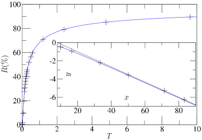
Figure 5: Acceptance rate $R$ of charge moves versus temperature. +, simulation results; solid line, Eq. 10. Inset, $y=\ln(R/\sqrt{T})$ against $x=1/T$. Numerical results approach the asymptote Eq. (11) of slope $-1/12$ (dashed line). A pair of opposite charges, box size $L=15$.

During motion of the charge, the field on $AB$ is modified to $-5q/6a^{2}\epsilon+\eta$. The energy difference between the two configurations is thus $\delta\mathcal{E}=qa(q/3a^{2}\epsilon-\eta)$. With the Metropolis algorithm when $\eta<q/3a^{2}\epsilon$ the trial is accepted with probability $\exp(-\delta\mathcal{E}/k_{B}T)$, otherwise it is automatically accepted. Computing the average over all values of $\eta$, we find the acceptance rate

$$R=\mathrm{erfc}\left(q/2\sqrt{3a\epsilon k_{B}T}\right).$$ (10)

We plot this function together with numerical results in Fig. 5. When $T$ is small, the asymptotic expansion of $\mathrm{erfc}$ gives

$$R=\sqrt{\frac{12T}{\pi}}e^{-1/12T}\bigl{(}1+\mathcal{O}\bigl{(}T\bigr{)}\bigr{)}.$$ (11)

Defining $y=\ln\bigl{(}R/\sqrt{T}\bigr{)}$ and $x=1/T$, we find an Arrhenius law for the acceptance rate $y=-x/12+\text{const.}+\mathcal{O}\bigl{(}1/x\bigr{)}$, which is illustrated in the inset of Fig. 5.

We conclude that particle motion becomes hard with this update scheme for $T<1/12$ due to a finite energy barrier. One of our aims in the rest of this paper will be to reduce the barrier so that the acceptance rate remains high even for temperatures $T\ll 1/12$.

IV.2 Field trails and string tension

Let us consider two closely separated charges with the electric field in equilibrium. The field has the usual dipolar form familiar from elementary electrostatics. What happens if we pull very hard on the positive charge so that the separation between the charges increases rapidly, without updating the plaquette degrees of freedom? During the motion of the particle each link traversed is modified by $q/a^{2}\epsilon$ leaving behind a “trail” of modified links (Fig. 6).

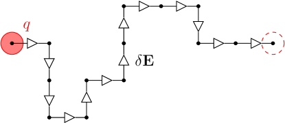
Figure 6: The field update produced by successive moves of a charge $q$ is a field string of intensity $\delta E=q/a^{2}\epsilon$ connecting the particle to its starting position (dashed circle). The trail remains as long as no plaquette update intervenes.

With time the field configuration will relax back to a dipolar form because of the updates of the plaquettes equilibrating the transverse field. However on a short time scale there are few plaquette updates, and dragging the charge along $r$ links costs an energy which we can estimate to be $r\gamma_{0}$, where

$$\gamma_{0}=q^{2}/2a\epsilon$$ (12)

is our estimate of the energy rise per link,

$$a^{3}\frac{\epsilon}{2}\left[\left(E-\frac{q}{a^{2}\epsilon}\right)^{2}-E^{2}\right]=-aqE+\frac{q^{2}}{2a\epsilon}$$

and $E$ has zero mean. There is a “string tension”, $\gamma_{0}$, pulling the particles back.

In the presence of an external electric field, a pair of opposite charges normally separates. A finite string tension implies that this mobility is suppressed. One must spend much numerical effort on updating the plaquettes in order to destroy the trail and stop particles backtracking. While the string tension is positive at low temperatures we will now argue that the thermodynamic tension $\gamma$ should become zero at a finite temperature: above it the mobility is high even at low frequencies of updates in the plaquettes.

Consider a trail joining two fixed test charges separated by a distance $r$ and let the length of the trail joining them be $\ell$. If $\ell\gg r$ we can estimate the number of such paths from the statistics of the path: $N_{\ell}=\mathcal{O}\bigl{(}z^{\ell}\bigr{)}$. $z$ is a connectivity constant characterizing the geometry of the walk. For a random walk $z=6$, for a self-avoiding walk $z=4.68$. We now estimate the free energy of the configuration as

$$F\approx\ell\gamma_{0}-k_{B}T\ell\ln z=\gamma\ell.$$ (13)

From this expression we can expect two distinct dynamic regimes for the algorithm. At low temperatures the tension $\gamma$ is positive and it is most favorable for the trail to remain short, $\ell\sim r$. The free energy for separating the charges is indeed linear and we have a phenomenon similar to confinement in gauge theories. This confinement is only destroyed by the dynamics of the plaquettes which slowly relaxes the trail into a dipolar field configuration. At temperatures higher than $T_{c}\sim\gamma_{0}/k_{B}\ln z\approx 0.3$ the line tension drops to zero and the particles become unconfined. Even without plaquette updates the particles remain mobile and can separate easily.

We also note that there is a very close analogy between this picture of roughening trails and the ($2+1$)-dimensional Hubbard model in the phase approximation, which can be expressed as a set of fluxes on a lattice Sørensen et al. (1992); Alet and Sørensen (2004). This model has two thermodynamic phases, one with tense field lines which are strongly suppressed, and a superconducting phase in which field lines proliferate. The transition occurs at a temperature $T\approx 0.33$.

In Fig. 4 we used a split in which one half of all updates try to move one of the two particles, and one half of updates modify a randomly chosen plaquette. The number of plaquettes ($3L^{3}\approx 10^{4}$) is much larger than the number of particles ($N=2$), so that a given plaquette is rarely updated, trail formation is probable. The diffusion coefficient of charges indeed drops at a crossover temperature $T_{c}\approx 0.2$ which qualitatively agrees with the above estimate.

How do we expect this trail-limited mobility to vary as a function of charge density? If a charge $i$ creates a trail, and a charge $j$ of the same sign crosses it, then $j$ will also feel the mean force mentioned above. If $j$ is now dragged back along the track of $i$, the field updates will erase the trail (Fig. 7). Afterwards, neither $i$ nor $j$ are linked to their initial positions. We thus expect that the effect of the trails is cut off at a distance comparable to the inter-particle spacing. Indeed we do find that the mobility increases on simulating systems of increasing charge densities. Thus in this paper we will concentrate on improving the efficiency of the algorithm at very low densities, working most often with samples containing just two charges.

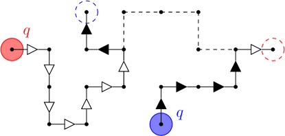
Figure 7: A second charge joins the string left by the charge of Fig. 6; it is dragged along the original path. Field updates then erase the previous trail (dashed line). The field strings no longer connect the particles to their respective starting sites (dashed circles).

In the next two sections we will modify the slaved updates in order to reduce the bare tension of strings. With a lower $\gamma_{0}$ we will lessen the crossover temperature $T_{c}\approx 0.2$ which results from the balance between energy and entropy expressed in Eq. (13). To efficiently simulate condensed matter systems, particles must remain highly mobile to much lower temperatures: $T=0.2$ corresponds to $l_{B}=a/4\pi T\approx 0.4~{}\text{\r{A}}$ (with $a=1~{}\text{\r{A}}$), whereas the Bjerrum length in water at room temperature is $l_{B}\approx 7~{}\text{\r{A}}$. Therefore we aim at lowering $T_{c}$ by a factor of approximately $20$.

V Extended charges

The expression (12) for the bare tension of the string is quadratic in the charge, $\gamma_{0}=q^{2}/2a\epsilon$. Let us now split the string between two particles into $K$ substrings; each substring carries a flux of $q/K\epsilon$. The bare tension of each substring will be $\gamma_{0}/K^{2}$, and that of the whole split string will be $K(\gamma_{0}/K^{2})=\gamma_{0}/K$.

In this section, to form split strings we spread the particles on cubes of side $w$; each site in the cube carries a subcharge of $q/w^{3}$, and when a particle moves the field is updated on the $w^{3}$ links crossed by each subcharge. We use values of $w$ ranging from 1 (the original algorithm) to 5, and measure the acceptance rate of particle updates. When we plot the rate as a function of $w^{3}T$ (Fig. 8) we find that all curves collapse, except at low temperatures for the two opposite charges due to pairing. We also simulated point charges with the coupled update proposed by Duncan, Sedgewick, and Coalson in Ref. Duncan et al. (2005) (hereafter denoted by “DSC”), and the acceptance rates collapse equally well.

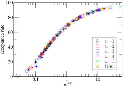
Figure 8: Acceptance rate of particle moves versus temperature for OCP (open symbols, $w=1$ to $5$) and a pair of charges (filled symbols, $w=1$ to $3$), temperature rescaled by $w^{3}$ (DSC, $7$).

The scaling of the acceptance rate in $w^{3}$ can be understood as follows: motion of each part of the particle is hindered by a barrier which varies as $(1/w^{3})^{2}$. The barriers are additive leading to a local barrier with an amplitude which varies as $1/w^{3}$.

When we plot mobility (determined from the dynamics of $\bar{\mathbf{E}}$) as a function of temperature, we find that the benefit obtained from charge spreading is not proportional to $w^{3}$; curves collapse on using a scaling with $w^{2}$, Fig. 9. The cross-section area of the extended charges is equal to $w^{2}$, so their field trails are made up from $K=w^{2}$ field lines of strength $q/a^{2}w^{2}\epsilon$. This gives a bare tension for the trail of $\gamma_{0}/w^{2}$. When trail formation limits mobility, the typical crossover temperature $T_{c}$ thus scales as $1/w^{2}$. This seems to indicate that the statistics of the paths and the connectivity constant do not change with $w$.

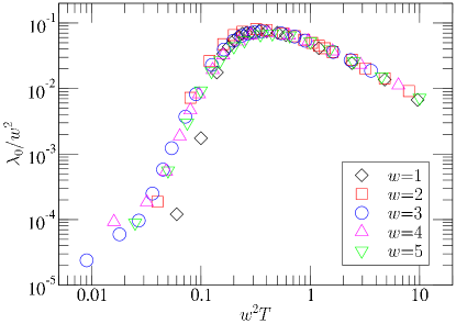
Figure 9: Mobility in OCP versus temperature ($N=2$, $L=15$). Each charge is spread on a $w$-site-side cube. Data collapse when temperature and $\lambda_{0}$ are scaled by $w^{2}$. For $T\rightarrow\infty$ the diffusion coefficient of particles is bound by $1~{}a^{2}\,(\text{sweep})^{-1}$: $D$ saturates and $\lambda_{0}\sim 1/T$.

To further confirm the idea that field trails are limiting mobility we introduced a new kind of field update: We define a cubic box of side $b$ centered on a site occupied by a particle, and then generate a worm update (Sec. II.2, and Ref. Levrel et al. (2005)) inscribed in the box. At each Monte Carlo step, the algorithm attempts one of three updates, either a particle move, a plaquette update, or a “local worm”. Since all choices are reversible detailed balance is verified.

Worm moves are known to lead to fast relaxation of the field, so these new “local worm updates” should allow one to spread out the field trails efficiently, concentrating the computational effort around charges, where the trails are formed. By introducing them in a 1:1 proportion with particle moves (with $b$ satisfying $b^{2}>w^{3}$), we expect to cancel the effective string tension. This computation is very expensive; one “local worm update” is far more costly than one particle update. We did not seek further optimization, and do not recommend this method for production of data with the algorithm.

We find that the crossover temperature $T_{c}$ of the mobility drop decreases with these local worm moves. In Fig. 10 the data superimpose if we rescale by a factor of $w^{3}$, implying that the trails are no longer dominating the dynamics. The $w^{3}$ scaling may be indicating that dynamics are now limited by the local barrier to particle hops described in Sec. IV.1.

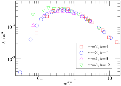
Figure 10: Mobility of OCP particles versus temperature at low density ($N=2$, $L=15$). Here local worm moves are introduced (see text), and now data are made collapse when scaled by $w^{3}$, showing that field trails have been removed, as opposed to data of Fig. 9.

The spreading of particles over several sites clearly modifies the interactions at short distance. One should introduce a hard core interaction for distances less than $wa$, corresponding to the diameter $r_{0}$ of the particles. Much of the interesting physics in soft condensed matter depends on the ratio of the Bjerrum length $l_{B}=e^{2}/4\pi\epsilon k_{B}T$ to the particle size. One is typically interested in the range $5<l_{B}/r_{0}<20$, which corresponds to $0.004<wT<0.02$. While we have succeeded in reducing the crossover temperature $T_{c}$ by a factor $1/w^{2}$ we have also changed the physical length scale by a factor $w$. The final result is only a factor $w$ improvement in $T_{c}$ when measured in physical units; a lattice algorithm suitable for condensed matter simulation would require $w\approx 20$. Such fine discretization has been used in lattice models to reproduce correctly thermodynamical properties of some systems Lock et al. (2004); Indrakanti et al. (2001). However for cases where this is not required, one might prefer to avoid such large $w$. We now explore methods of moving charges which do not require permanent spreading so that the effective length scale in the simulation is not modified.

VI Temporary charge spreading

There is a direct way of reconciling the requirements that charges are extended during their motion but otherwise pointlike: Before moving a particle, one should first spread its charge evenly onto neighboring sites, then move all subcharges as a block, and finally bring them back together (see Fig. 11). This defines a charge move involving three substeps.

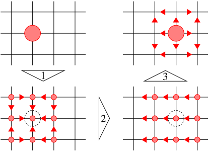
Figure 11: Temporary spreading of charge (here with $w=3$). First step, spread the charge to $w^{3}$ sites. Second step, move the extended set of charges. Third step, inverse of the first; charge fractions collapse back to a point. The overall field update is the sum of the individual steps.

Each step consists of a set of currents. When a charge is split a current $\mathbf{j}^{(1)}$ flows from the central site. Motion of the particle generates a current, $\mathbf{j}^{(2)}$. When the charge is collapsed to a point a current $\mathbf{j}^{(3)}$ flows from the neighboring sites back to the center. To maintain the constraint of Gauss’s law, each of these currents $\mathbf{j}^{(\alpha)}$ is associated with a field update $\delta\mathbf{E}^{(\alpha)}=-\mathbf{j}^{(\alpha)}\delta t/\epsilon$. For step 2, the current on each modified link is $j^{(2)}=q/w^{3}a^{2}\delta t$, as above. During step 1 the values $j_{i}^{(1)}$ of the current on links $\{i\}$ are under-determined, they are constrained only by charge conservation Eq. (3). We thus additionally require that $\sum_{i}\bigl{(}j_{i}^{(1)}\bigr{)}^{2}/2$ be a minimum, giving a unique, reversible recipe for the current. We solve for $\mathbf{j}^{(1)}$ by minimizing the functional

$$\mathcal{F}=\int\frac{\left(\mathbf{j}^{(1)}\right)^{2}}{2}-\Lambda\left(\mathrm{div}\,\mathbf{j}^{(1)}+\frac{\delta\rho^{(1)}}{\delta t}\right).$$

The current is the solution of a Poisson-type problem,

$$\mathbf{j}^{(1)}=-\mathrm{grad}\,\Lambda\quad\text{and}\quad\nabla^{2}\Lambda=\frac{\delta\rho^{(1)}}{\delta t}$$

with $\mathbf{j}^{(1)}\cdot\mathbf{n}=0$ on the boundary of the spread charge. The solution to this equation is computed once during initialization of the simulation and stored in a lookup table. Step 3 is the exact reverse of step 1, $\mathbf{j}^{(3)}=-\mathbf{j}^{(1)}$. On adding the fields $\mathbf{j}^{(1)}$, $\mathbf{j}^{(2)}$, and $\mathbf{j}^{(3)}$ we find a flow going from the starting site to the final site, and taking several paths.

If now we simulate our test system using this version of the algorithm and plot the mobility of particles versus temperature (Fig. 12), we find practically the same results as in Fig. 9. The crossover temperature scales with $1/w^{2}$. The advantage is that the particles are still pointlike unlike Sec. V. Thus we have improved the lowest temperatures efficiently accessible by a factor of $w^{2}$ without changing the physically important length scale.

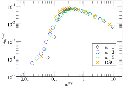
Figure 12: Mobility of temporarily spread charges versus temperature. OCP, $N=2$, $L=15$. The mobility with no spreading ($w=1$) is also given. Data are rescaled by $w^{2}$ (DSC, $3.77$).

The method has the advantage of both simplicity and generality.

• A small Poisson equation is solved once before starting simulation in order to determine the “current map”.

• One is free to choose as an intermediate state an arbitrary charge cloud.

We note that temporary spreading includes the Monte Carlo algorithm of DSC as a special case, it is sufficient to consider the six nearest neighbors of a site, plus the site itself, as the volume over which the charge is to be spread. Each site thus gets one seventh of the total charge $q$, which explains the scaling of acceptance rate in Fig. 8. The result of steps 1 through 3 of Fig. 11 yields a current $3q/7a^{2}\delta t$ on the center link and $q/7a^{2}\delta t$ around the four plaquettes adjacent to it. The curve obtained by using DSC updates collapses with the others in Fig. 12, when scaled by $49/13=3.77$ which comes from a simple estimate of the bare string tension. However in our simulations we have not implemented the additional step of simulating the update with heat bath rather than Metropolis update.

Rather than performing three successive steps, another implementation of the temporary spreading consists in precomputing the total “map” of currents $\mathbf{j}^{(1)}+\mathbf{j}^{(2)}+\mathbf{j}^{(3)}$. Such an implementation is faster, avoiding multiple updates of the same links through steps 1–3. However, keeping the three sub-steps distinct allows one to perform several intermediate updates of step 2, moving the particle a large distance before “recondensing” it to a point, as follows. Consider a (starting) configuration $\mathcal{C}_{\text{S}}$ of the system. We randomly choose one particle and spread its charge unconditionally; the field is updated accordingly and we label the new configuration as $\mathcal{C}_{i=0}$; the energy difference between $\mathcal{C}_{\text{S}}$ and $\mathcal{C}_{0}$ is stored. Then we successively try $d$ moves of that particle in random directions, which lead to configurations $\mathcal{C}_{i}$, $1\leqslant i\leqslant d$. The field is updated and trials are accepted with the Metropolis probability

$$m(\Delta\mathcal{E})=\min\left(1,\exp\left(-\frac{\Delta\mathcal{E}}{k_{B}T}\right)\right)$$

where $\Delta\mathcal{E}$ is the energy difference between the tried and current configurations. Finally the charge is condensed, yielding the ending state $\mathcal{C}_{\text{E}}$, and the whole update is accepted with probability

$$p_{\text{acc}}=m\bigl{(}\Delta\mathcal{E}(\mathcal{C}_{\text{S}}\rightarrow\mathcal{C}_{0})+\Delta\mathcal{E}(\mathcal{C}_{d}\rightarrow\mathcal{C}_{\text{E}})\bigr{)}.$$

The method saves computational effort, for each series of $d$ moves there are only one spreading and one condensation steps; there would be $d$ such steps if the procedure of local hopping of Fig. 11 were used.

To prove that detailed balance is obtained, consider an instance of such an update. Its global probability is

$$p(\mathcal{C}_{\text{S}}\rightarrow\mathcal{C}_{\text{E}})=p_{\text{acc}}\prod_{i=0}^{d-1}p(\mathcal{C}_{i}\rightarrow\mathcal{C}_{i+1}).$$

The probability of the ($i+1$)th step is

$$p(\mathcal{C}_{i}\rightarrow\mathcal{C}_{i+1})=\\ \begin{cases}\displaystyle\frac{1}{6}\,m\bigl{(}\Delta\mathcal{E}(\mathcal{C}_{i}\rightarrow\mathcal{C}_{i+1})\bigr{)}&\text{if $\mathcal{C}_{i}\neq\mathcal{C}_{i+1}$ (accepted trial),}\\ \displaystyle 1-\frac{1}{6}\sum_{\alpha^{\prime}}m\bigl{(}\Delta\mathcal{E}(\mathcal{C}_{i}\overset{\alpha^{\prime}}{\rightarrow})\bigr{)}&\text{if $\mathcal{C}_{i}=\mathcal{C}_{i+1}$ (rejected trial),}\end{cases}$$

where the sum runs over the six directions of space, and $\Delta\mathcal{E}(\mathcal{C}_{i}\overset{\alpha^{\prime}}{\rightarrow})$ is the energy change corresponding to a trial move in the $\alpha^{\prime}$ direction from configuration $i$. The probability of the reverse update reads

$$p(\mathcal{C}_{\text{E}}\rightarrow\mathcal{C}_{\text{S}})=p^{\prime}_{\text{acc}}\prod_{i=0}^{d-1}p(\mathcal{C}_{i+1}\rightarrow\mathcal{C}_{i}),$$

where the global acceptance probability is

$$p^{\prime}_{\text{acc}}=m\bigl{(}\Delta\mathcal{E}(\mathcal{C}_{\text{E}}\rightarrow\mathcal{C}_{d})+\Delta\mathcal{E}(\mathcal{C}_{0}\rightarrow\mathcal{C}_{\text{S}})\bigr{)}.$$

When $\mathcal{C}_{i}=\mathcal{C}_{i+1}$,

$$\frac{p(\mathcal{C}_{i}\rightarrow\mathcal{C}_{i+1})}{p(\mathcal{C}_{i+1}\rightarrow\mathcal{C}_{i})}=1=\exp\left(-\frac{\Delta\mathcal{E}_{i\rightarrow i+1}}{k_{B}T}\right),$$

when $\mathcal{C}_{i}\neq\mathcal{C}_{i+1}$,

$$\frac{p(\mathcal{C}_{i}\rightarrow\mathcal{C}_{i+1})}{p(\mathcal{C}_{i+1}\rightarrow\mathcal{C}_{i})}=\frac{m(\Delta\mathcal{E}_{i\rightarrow i+1})}{m(\Delta\mathcal{E}_{{i+1}\rightarrow i})}=\exp\left(-\frac{\Delta\mathcal{E}_{i\rightarrow i+1}}{k_{B}T}\right),$$

and

$$\frac{p_{\text{acc}}}{p^{\prime}_{\text{acc}}}=\exp\left(-\frac{\Delta\mathcal{E}(\mathcal{C}_{\text{S}}\rightarrow\mathcal{C}_{0})+\Delta\mathcal{E}(\mathcal{C}_{d}\rightarrow\mathcal{C}_{\text{E}})}{k_{B}T}\right),$$

so that

$$\frac{p(\mathcal{C}_{\text{S}}\rightarrow\mathcal{C}_{\text{E}})}{p(\mathcal{C}_{\text{E}}\rightarrow\mathcal{C}_{\text{S}})} =\exp\left(-\frac{\Delta\mathcal{E}_{\text{S}\rightarrow 0}+\overset{d-1}{\underset{i=0}{\sum}}\Delta\mathcal{E}_{i\rightarrow i+1}+\Delta\mathcal{E}_{d\rightarrow\text{E}}}{k_{B}T}\right)$$

$$=\exp\left(-\frac{\mathcal{E}(\mathcal{C}_{\text{E}})-\mathcal{E}(\mathcal{C}_{\text{S}})}{k_{B}T}\right).$$

To check that the mobility is not changed when these long-ranged particle moves are used, we simulated our test system with them, fixing $d=15$. Regarding time units, one such update amounts to $d$ elementary Monte Carlo steps. On Fig. 13 we find that the mobility of charges is very little affected by the use of long distance particle updates. However CPU cost is reduced, as is shown in next section.

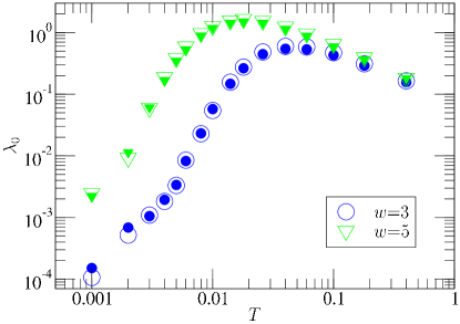
Figure 13: Mobility of temporarily spread charges versus temperature. OCP, $N=2$, $L=15$. Open symbols, one trial move per update. Filled symbols, $d=15$ trial moves per update.

	Permanent spreading			Temporary spreading, precomputed current			Temporary spreading, long-ranged particle moves
	$\lambda_{0}~{}[\text{(VS)}^{-1}]$	$t_{\text{CPU}}~{}[\text{s}]$	efficiency [s-1]	$\lambda_{0}~{}[\text{(VS)}^{-1}]$	$t_{\text{CPU}}~{}[\text{s}]$	efficiency [s-1]	$\lambda_{0}~{}[\text{VS}^{-1}]$	$t_{\text{CPU}}~{}[\text{s}]$	efficiency [s-1]
$w=1$	0$\mathstrut\times 10^{-4}$	71	$0$	0$\mathstrut\times 10^{-4}$	71	$0$	0$\mathstrut\times 10^{-4}$	71	$0$
$w=3$	$1.3\times 10^{-3}$	160	$0.49$	$5\times 10^{-2}$	592	$5$	$6\times 10^{-2}$	233	$15$
$w=5$	$1.4\times 10^{-2}$	582	$1.4$	1.3$\mathstrut\times 10^{-4}$	2372	$33$	1.2$\mathstrut\times 10^{-4}$	912	$79$

Table 1: Comparison of the various algorithms presented. $\lambda_{0}$, rate at which field configurations decorrelate, in simulation units. $t_{\text{CPU}}$, duration of the 60 000 VS simulation. Efficiency, real rate at which configurations decorrelate, given by $\lambda_{0}\times 60~{}000/t_{\text{CPU}}$. $w=1$ stands for the single-link field update, displayed for execution time comparisons.

VII Optimization

In Secs. V and VI, we presented several ways of updating the electric field during charge motion. We also measured the mobility of charges. However, the rates $\lambda_{0}$ have been computed in simulation units; time is expressed in Monte Carlo trials. As a function of their complexities, the different kinds of update require different computational effort. In order to choose the best parameters for a simulation we should express the efficiency of the various versions of the algorithm in terms of CPU time.

We simulated $N=2$ mobile charges in a box of size $L=15$. $T=0.01$ when charges are pointlike (temporary spreading) and $T=0.01/w$ when spread. This set of parameters is representative for simulating a monovalent ion in water. At each elementary Monte Carlo step (MCS), we try a particle move with probability $p_{1}=50\%$, and a plaquette update with probability $p_{2}=50\%$. We define a “volume sweep” (VS) $1~{}\text{VS}=L^{3}~{}\text{MCS}$. $60~{}000~{}\text{VS}\gtrsim 2\times 10^{8}~{}\text{MCS}$ are performed after equilibration. Temporary spreading was implemented in both ways of Sec. VI: first, with steps 1 to 3 of Fig. 11 summed up and stored in a single lookup table; second, with multiple steps 2 between each spreading-and-recondensing pair of events.

In Table 1 we compare the efficiency of the various updates introduced in this paper. We used a Pentium 4 at 2.6 GHz; our C++ code was compiled with an Intel compiler. We conclude that the most efficient field update is the temporary spreading of charges on $w=5$ cubes. At $T=0.01$, the mobility reached with $w=5$ is close to the maximum possible value: $D\approx 0.15~{}a^{2}\,(\text{sweep})^{-1}$ is rather close to saturation. We thus do not expect benefit from further spreading of charges ($w\geqslant 6$). As noted previously, both versions of temporary spreading yield almost the same mobility. The difference between the two is CPU time: long-ranged particle moves lead to a faster algorithm thanks to fewer spreading and recondensing steps. This version should thus be used for free charges.

Finally, we have checked that our results remain valid for higher densities. We applied our optimal solution (temporary spreading over $5^{3}$ sites) to simulate OCPs containing $N=14$, $34$, and $336$ positive charges, which, respectively, corresponds to number densities $n\approx 0.4\%$, $1\%$, and $10\%$.

In Sec. III, we calculated a relationship according to which $\lambda_{0}\propto n\mu$. This was for $\lambda_{0}$ in physically relevant units of time, like particle sweeps (PS): the effects of each charge add up, hence the factor of $n$. Here we measure time in volume sweeps (VS), and work at constant numerical effort, split amongst particles: the more charges there are, the fewer trials each one does. $1~{}\text{VS}=0.5/n~{}\text{PS}$, so that $\lambda_{0}[\text{in (VS)}^{-1}]=0.5\lambda_{0}[\text{in (PS)}^{-1}]/n$ is directly proportional to $\mu$. Plotting mobility against temperature in Fig. 14 we find that lowest mobility is found at the lowest density; at high density $\mu$ decreases, possibly because of steric hindrance, but remains greater than when $N=2$. Thus using our algorithm is always at least as efficient as displayed in Table 1.

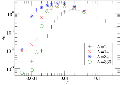
Figure 14: Mobility of charges temporarily spread on $w=5$ cubes, for an OCP at various densities ($n=N/L^{3}$ with $L=15$).

VIII Conclusion

The original version of the local Monte Carlo algorithm suffers from two problems at low temperature. First the acceptance rate becomes low due to a energy barrier for particle motion. A more serious problem is that the mobility falls even faster than the acceptance rate. We understand this fall in mobility by considering the tension of the strings left behind particles as they move. The different scaling of the acceptance rate and the mobility with the spreading parameter $w$ is a clear demonstration that two different mechanisms are important in limiting particle motion.

Simple modifications to the algorithm reduce the energy barrier for single particle moves, but also the string tension. The algorithm is then suitable for simulation of lattice models of Coulomb interacting particles. Examples include the restricted primitive model for electrolytes, or lattice models of polyelectrolytes.

Combination of the update methods used in this article with the worm update for the transverse field due to Alet and Sørensen Alet and Sørensen (2004) can lead to efficient codes for the simulation of charge systems at high dilution: Consider a set of $N$ charges in a simulation box of size $L$. It takes a computational effort of order $NL^{2}$ for these particles to diffuse the system size. We have already shown Levrel et al. (2005) that the $2L^{3}$ tranverse degrees of freedom of the lattice can be integrated over in $\mathcal{O}\bigl{(}1\bigr{)}$ sweeps of the worm algorithm with an effort scaling as $L^{3}$. One can thus equilibrate a dilute system of mobile charges with a computer effort which scales as $(NL^{2}+L^{3})$.

The time moving the particles dominates the time needed for the electrostatic integration if $N>L$, or if the density $n>1/L^{2}$; when $L$ is large the algorithm remains efficient even for very dilute charges. It is thus well suited to the study of heterogenous systems such as surfaces and polyelectrolytes.

References

- Frenkel and Smit (2002) D. Frenkel and B. Smit, Understanding molecular simulation (Academic, New York, 2002), chap. 12.
- Shan et al. (2005) Y. Shan, J. L. Klepeis, M. P. Eastwood, R. O. Dror, and D. E. Shaw, J. Chem. Phys. 122, 054101 (2005).
- Perram et al. (1988) J. W. Perram, H. G. Petersen, and S. W. de Leeuw, Mol. Phys. 65, 875 (1988).
- Maggs and Rossetto (2002) A. C. Maggs and V. Rossetto, Phys. Rev. Lett. 88, 196402 (2002).
- Duncan et al. (2005) A. Duncan, R. D. Sedgewick, and R. D. Coalson, Phys. Rev. E 71, 046702 (2005).
- Rottler and Maggs (2004) J. Rottler and A. C. Maggs, J. Chem. Phys. 120, 3119 (2004).
- Panagiotopoulos and Kumar (1999) A. Z. Panagiotopoulos and S. K. Kumar, Phys. Rev. Lett. 83, 2981 (1999).
- Panagiotopoulos (2000) A. Z. Panagiotopoulos, J. Chem. Phys. 112, 7132 (2000).
- Moghaddam and Panagiotopoulos (2003) S. Moghaddam and A. Z. Panagiotopoulos, J. Chem. Phys. 118, 7556 (2003).
- Carmesin and Kremer (1988) I. Carmesin and K. Kremer, Macromolecules 21, 2819 (1988).
- Binder and Paul (1997) K. Binder and W. Paul, J. Polym. Sci. Part B: Polym. Phys. 35, 1 (1997).
- Maggs (2002) A. C. Maggs, J. Chem. Phys. 117, 1975 (2002).
- Maggs (2004) A. C. Maggs, J. Chem. Phys. 120, 3108 (2004).
- Levrel et al. (2005) L. Levrel, F. Alet, J. Rottler, and A. C. Maggs, Pramana 64, 1001 (2005), Proceedings of the 22nd IUPAP international conference on statistical physics (StatPhys 22).
- Novotny (1995) M. A. Novotny, Phys. Rev. Lett. 74, 1 (1995).
- Sørensen et al. (1992) E. S. Sørensen, M. Wallin, S. M. Girvin, and A. P. Young, Phys. Rev. Lett. 69, 828 (1992).
- Alet and Sørensen (2004) F. Alet and E. S. Sørensen, Phys. Rev. B 70, 024513 (2004).
- Lock et al. (2004) C. S. Lock, S. Moghaddam, and A. Z. Panagiotopoulos, Fluid Phase Equilib. 222-223, 225 (2004).
- Indrakanti et al. (2001) A. Indrakanti, J. K. Maranas, A. Z. Panagiotopoulos, and S. K. Kumar, Macromolecules 34, 8596 (2001).