Strategy correlations and timing of adaptation in Minority Games

Abstract

We study the role of strategy correlations and timing of adaptation for the dynamics of Minority Games, both simulationally and analytically. Using the exact generating functional approach à la De Dominicis we compute the phase diagram and the behaviour of batch and on-line games with correlated strategies, complementing exisiting replica studies of their statics. It is shown that the timing of adaptation can be relevant; while conventional games with uncorrelated strategies are nearly insensitive to the choice of on-line versus batch learning, we find qualitative differences when anti-correlations are present in the strategy assignments. The available standard approximations for the volatility in terms of persistent order parameters in the stationary ergodic states become unreliable in batch games under such circumstances. We then comment on the role of oscillations and the relation to the breakdown of ergodicity. Finally, it is discussed how the generating functional formalism can be used to study mixed populations of so-called ‘producers’ and ‘speculators’ in the context of the batch minority games.

1 Introduction

The collective behaviour of interacting heterogeneous and adaptive agents has attracted a substantial amount of attention in the statistical physics communtity in recent years. The general aim is to understand how complex macroscopic co-operation can emerge from the underlying microscopic laws that govern the behaviour of the individual agents. The minority game (MG) ChalZhan97 is probably one of the most studied models in this context. It describes an ensemble of traders who at each time step receive a piece of public information and react by either buying or selling. Learning from past experience, the aim of the individual agent is to be in the minority at each round of the game, i.e. to buy when most of the traders are selling and vice versa. To take their trading decisions the agents employ strategies assigned randomly at the start of the game and then kept fixed. These effectively act as look-up tables providing a map from the observed public information onto a binary trading decision. At each time step the individual agent employs the strategy in his or her pool he or she believes will maximise their potential payoff. In order to measure the performance of their strategies they allocate virtual points to each of their strategies, increasing the score of strategies that would have yielded a correct minority decision.

Thanks to the simplicity of the microscopic equations of motion and because of analogies to models of spin-glasses and neural networks, analytical progress can be made using both static and dynamical methods of statistical mechanics. It has been found that the relevant control parameter for MGs is the ratio $\alpha=P/N$ of the number $P$ of possible values for the external information over the number of players $N$. A phase transition between an ergodic phase at high $\alpha$ and non-ergodic states below a critical value $\alpha_{c}$ has been identified and analytical expressions for the macroscopic order parameters characterising the different states have been obtained ChalMarsZhan00 ; ChalMarsZecc00 ; MarsChalZecc00 ; GarrMoroSher00 ; HeimCool01 ; MarsChal01 . While some order parameters in the ergodic phase can be computed in the thermodynamic limit $N\to\infty$ without making any approximations, the dynamics of the game in its non-ergodic phase at low values of $\alpha$ is not yet fully understood. Furthermore the calculation of a key observable of the MG, the magnitude of the overall market fluctuations or so-called volatility, is up to now restriced to approximations both in dynamical approaches and in static replica analyses HeimCool01 ; ChalMarsZecc00 .

In the original setup of the MG the strategies assigned to a given agent were completely uncorrelated and the information fed to the agents was based on the real history of the market dynamics ChalZhan97 ; SaviManuRiol99 . Also, updates of the virtual scores of the agents’ strategies were performed after each round of the game, and their relative success re-assessed before each trading decision, i.e. agents could switch strategies between any two successive rounds of the game. Such variants of the MG with score updates at every round of the game are generally referred to as ‘on-line’ games. It was realised that no qualitative changes in the overall behaviour occured when the stream of information was replaced by random inputs at each time step Cava99 . Hereafter we shall therefore distinguish between on-line games with ‘real’ or ‘random’ market history, respectively. It is technically much easier to deal with the case of ‘random’ history so henceforth we concentrate on this version (see however the recent work Cool04 for a generating functional analysis of MGs with real market histories). Early studies showed only slight differences between on-line MGs with uncorrelated strategies and corresponding games in which the agents effectively sample a large set of information patterns before updating the scores of their strategies. This amounts to replacing the inflowing information by an averaging procedure over all possible values of the pieces of information to yield an effective interaction between the agents; such models are known as ‘batch’ minority games. On the technical level, using this effective interaction, the dynamics of batch MGs are much easier to study than their on-line counterparts, and hence most current dynamical studies are concerned with batch versions of the MG HeimCool01 ; HeimDeMa01 ; DeMaGiarMose03 ; DeMa03 ; GallCoolSher03 ; Gall05 . Also, here we restrict ourselves to the case of deterministic decision making; a stochastic extension is straightforward to consider CoolHeimSher01 , but complicates the detailed mathematics of the analysis. Reviews on the MG can be found in Coolenreview ; Moro04 ; note also the recently published textbooks MGbook1 ; MGbook2 .

In this paper we extend the generating functional analysis of batch and on-line games with uncorrelated strategies as presented in HeimCool01 ; CoolHeim01 to the case of correlated and anti-correlated strategies. The purpose is twofold, firstly we provide an analysis of the dynamics of such MGs with so-called ‘diversified’ strategies and complement the study of their statics previously presented by other authors in ChalMarsZhan00 . Secondly, we find that in the presence of anti-correlated strategies significant differences in the global behaviour of batch and on-line MGs are present, i.e. that the the overall performance of the system strongly depends on the timing of adapation of the agents. This effect is small in the case of conventional MGs with uncorrelated strategies, but becomes magnified as the degree of anti-correlation in the strategy assignments is increased. We also demonstrate that some approximations which reproduce the the volatility of batch MGs with uncorrelated strategies with good accuracy, and are hence often considered to be standard, become inaccurate in games with highly anti-correlated stategies. We then discuss the effects of strategy correlations on the sensitivity to initial conditions and comment on the relation between the global oscillations and the breakdown of ergodicity in batch and on-line MG with different strategy correlations. As a by-product of the generating functional analysis of the dynamics of games with general distributions of correlation parameters we finally study the case of bi-modal distributions, corresponding to a mixed population of so-called ‘speculators’ and ‘producers’

2 Model Definitions

The MG describes the decision making dynamics of $N$ interacting agents, $i=1,\dots,N$. At each round $\ell$ of the game all agents are given the same external information $I(\ell)$ taken from a set of $P$ elements. They utilise this information to determine an action by choosing from one of a personal set of $S$ strategies whose operation on the information yields a decision. Simulations have shown that restriction to $S=2$ strategies per agent yields characteristic behaviour. It also simplifies the analysis. Hence we restrict the further discussion here to this case. We also simplify the choices of the space of information and character of the decisions. Hence here we take each agent to hold two $P$-dimensional strategy vectors ${\mbox{\boldmath$R$}}_{ia}=(R_{ia}^{1},\dots,R_{ia}^{P})$, $a=\pm 1$, with each component $R_{ia}^{\mu}$ chosen randomly from the set $\{-1,1\}$ at the beginning of the game and thereafter fixed and the information to be given by an integer $\mu(\ell)$ chosen randomly and independently at each step $\ell$ from the set $\{1,\dots,P=\alpha N\}$. Then the strategies act as look up tables for deciding ‘trading’ action, yielding output $R^{\mu(\ell)}_{ia}$. If player $i$ decides to use strategy $a^{*}_{i}(\ell)$ at round $\ell$ of the game his or her trading action will be $b_{i}(t)=R_{i{a_{i}^{*}}(\ell)}^{\mu(\ell)}$. The re-scaled total bid at stage $\ell$ is then defined as $A(\ell)=N^{-1/2}\sum_{i}b_{i}(\ell)$. In order to decide which of their two strategies to use at any given time each players keeps a record of the relative performance of his or her strategies. A payoff value $p_{ia}(\ell)$ is assigned to each strategy and updated every $M$ time steps according to

$$p_{ia}(\ell+M)=p_{ia}(\ell)-\frac{\Gamma}{\sqrt{N}}\sum_{\ell^{\prime}=\ell}^{\ell+M-1}R_{ia}^{\mu(\ell^{\prime})}A(\ell^{\prime}).$$ (1)

In between the updates the scores $p_{ia}$ are kept constant. $\Gamma>0$ is a learning rate and of order ${\cal O}(N^{0})$, introduced for convenience CoolHeim01 . Note that the minus sign in the update prescription ensures that strategies which predict correct minority decisions are rewarded. At each round player $i$ then plays the strategy in his or her arsenal with the highest relative score, i.e. $a^{*}_{i}(\ell)={\rm sgn}[q_{i}(\ell)]$, where $q_{i}(\ell)=\frac{1}{2}(p_{i,1}(\ell)-p_{i,-1}(\ell))$ is the point difference of player $i$’s strategies at time $\ell$. Upon introduction of ${\mbox{\boldmath$\omega$}}_{i}=({\mbox{\boldmath$R$}}_{i,1}+{\mbox{\boldmath$R$}}_{i,-1})/2$ and ${\mbox{\boldmath$\xi$}}_{i}=({\mbox{\boldmath$R$}}_{i,1}-{\mbox{\boldmath$R$}}_{i,-1})/2$ the update rule (1) can be compactified to

$$q_{i}(\ell+M) = q_{i}(\ell)-\frac{\Gamma}{\sqrt{N}}\sum_{\ell^{\prime}=\ell}^{\ell+M-1}\xi_{i}^{\mu(\ell^{\prime})}$$ (2)

$$\times\bigg{\{}N^{-1/2}\sum_{j}\left(\omega_{j}^{\mu(\ell^{\prime})}+\xi_{j}^{\mu(\ell^{\prime})}s_{j}(\ell^{\prime})\right)\bigg{\}}.$$

Here we have introduced the shorthand notation $s_{i}(\ell)={\rm sgn}[q_{i}(\ell)]$, we will also abbreviate ${\mbox{\boldmath$\Omega$}}=N^{-1/2}\sum_{j}{\mbox{\boldmath$\omega$}}_{j}$. The case $M=1$ (where strategy scores are updated at every time step) is referred to as the on-line model. For $M\geq{\cal O}(\alpha N)$ one expects (and simulations confirm) the behaviour of the system to be the same as that for the so-called batch version in which the sum over the actual values $\mu(\ell^{\prime})$ is replaced by an average over the set $\mu\in\{1,\dots,\alpha N\}$:

$$q_{i}(t+1) = q_{i}(t)-\frac{\Gamma}{N}\sum_{\mu=1}^{\alpha N}\xi_{i}^{\mu}\big{\{}\sum_{j}\left(\omega_{j}^{\mu}+\xi_{j}^{\mu}s_{j}(t)\right)\big{\}}.$$ (3)

Note that an appropriate re-scaling of time is implied, as one batch time step corresponds to ${\cal O}(\alpha N)$ on-line steps. Introducting the notation $J_{ij}=\Gamma{\mbox{\boldmath$\xi$}}_{i}\cdot{\mbox{\boldmath$\xi$}}_{j}/N$ and $h_{i}=\Gamma{\mbox{\boldmath$\xi$}}_{i}\cdot{\mbox{\boldmath$\Omega$}}/\sqrt{N}$ the batch update rule (3) can be written compactly as

$$q_{i}(t+1)=q_{i}(t)-h_{i}-\sum_{j}J_{ij}s_{j}(t).$$ (4)

In the original game the strategies are chosen without correlations between the agents and also independently within the set of strategies of a fixed agent $i$, i.e. one has

$$\overline{R_{ia}^{\mu}R_{jb}^{\nu}}=\delta_{ij}\delta_{ab}\delta_{\mu\nu},$$ (5)

where $\overline{\cdots}$ denotes an average over the disorder, i.e. over the space of strategy assignments. In this paper, we will consider cases of correlated strategy vectors ${\mbox{\boldmath$R$}}_{i,-1}$ and ${\mbox{\boldmath$R$}}_{i,1}$ of a fixed agent $i$. Specifically we generalize the standard case to a situation in which $R_{i1}^{\mu}=R_{i2}^{\mu}$ with probability $\rho_{i}\in[0,1]$ for any given $i$ and $\mu$ (and $R_{i1}^{\mu}\neq R_{i2}^{\mu}$ with probability $1-\rho_{i}$, recall that the $R_{ia}^{\mu}$ take only values $-1$ and $1$). The joint probability distribution of $R_{i1}^{\mu}$ and $R_{i2}^{\mu}$ is then given by

$$P(R_{i1}^{\mu}=x,R_{i2}^{\mu}=y) = \frac{\rho_{i}}{2}\left(\delta_{x,-1}\delta_{y,-1}+\delta_{x,1}\delta_{y,1}\right)$$ (6)

$$+\frac{1-\rho_{i}}{2}\left(\delta_{x,-1}\delta_{y,1}+\delta_{x,1}\delta_{y,-1}\right).$$

The standard situation of independent strategies is covered as the special case $\rho_{i}=1/2$ for all players $i$. On the other hand, if $\rho_{i}=1$, then player $i$ holds two identical strategy vectors, whereas for $\rho_{i}=0$ he or she has two opposite strategies, ${\mbox{\boldmath$R$}}_{i,-1}=-{\mbox{\boldmath$R$}}_{i,1}$. Allowing the correlation parameter $\rho_{i}$ to depend on $i$ adds another layer of heterogeneity to the ensemble of agents: not only are their strategies chosen at random and hence are heterogeneous across the group of $N$ players, but also the probability distribution from which they are drawn may be different for different agents. We will assume that each $\rho_{i}$ is randomly and independently drawn from a distribution $P(\rho)$, so that, for example, $P(\rho)=\delta(\rho-1/2)$ corresponds to the standard game, with $\rho_{i}=1/2$ for all $i$. Some of our results presented below have been summarized in the short paper SherGall03 . The statics of MGs with correlated strategies were first studied using replica methods in ChalMarsZhan00 . Numerical results are also found in GarrMoroSherr01 , and in YipHuiLoJohn03 , where an effective correlation between the assigned strategies was introduced upon biasing the $\{R_{ia}^{\mu}\}$ towards one of the binary entries.

Let us finally, in this section, introduce the volatility, $\sigma^{2}$, of the market. It describes the variance of the total re-scaled market bid $A$, and can be defined as the following long-time average:

$$\sigma^{2}=\lim_{\tau\to\infty}\tau^{-1}\sum_{\ell\leq\tau}A(\ell)^{2}.$$ (7)

In on-line models the relevant average over the stochasticity of the information is to be performed, as $A(\ell)$ depends on both the score valuations $\{q_{i}(\ell)\}$ and the value of the external information $\mu(\ell)$. In deterministic batch games this average is replaced by one over $\mu$

$$\sigma^{2}=\lim_{\tau\to\infty}\tau^{-1}\sum_{t\leq\tau}P^{-1}\sum_{\mu=1}^{P}(A^{\mu}(t))^{2},$$ (8)

where $A^{\mu}(t)=\Omega^{\mu}+N^{-1/2}\sum_{j}\xi_{j}^{\mu}s_{j}(t)$. The volatility is a measure for the global efficiency of the market; if $\sigma^{2}=0$ supply and demand are always matched ($A=0$) and trading is fully efficient. Non-zero volatilities however indicate mismatches between the numbers of buyers and sellers, and hence imply inefficient markets. For the mathematical analysis of batch MGs it is also convenient to introduce the volatility matrix $\Xi$ HeimCool01

$$\Xi_{tt^{\prime}}=P^{-1}\sum_{\mu=1}^{P}A^{\mu}(t)A^{\mu}(t^{\prime}).$$ (9)

Note that $\sigma^{2}=\lim_{\tau\to\infty}\tau^{-1}\sum_{t\leq\tau}\Xi_{tt}$, and that stochastic trading with $s_{i}(t)=\pm 1$ taken randomly and independently at any time step $t$ would result in $\Xi_{tt^{\prime}}=\frac{1}{2}(1+\delta_{tt^{\prime}})$ in the thermodynamic limit. In particular $\sigma^{2}=1$ is the so-called random trading limit.

3 Generating functional and effective single-agent process for the batch game

We will now turn to the generating functional analysis of the batch process (3). The calculation is an extension of the analysis of the standard game presented in HeimCool01 .

3.1 Generating functional and disorder average

The moment generating functional corresponding to the batch process of Eq. (3) reads

$$Z[{\mbox{\boldmath$\psi$}}] = \int d\mathbf{q}\,p_{0}(q(0))\exp\left(i\sum_{it}\psi_{i}(t)s_{i}(t)\right)$$ (10)

$$\prod_{it}\delta\left(q_{i}(t+1)-q_{i}(t)+\sum_{j}J_{ij}s_{j}(t)+h_{i}-\theta_{i}(t)\right),$$

where we have introduced the usual source term containing the field variables $\{\psi_{i}(t)\}$. The $\{\theta_{i}(t)\}$ are additional perturbation fields, introduced to generate response functions, and $p_{0}(q(0))$ denotes the probability distribution of the initial score differences $q(0)=(q_{1}(0),\dots,q_{N}(0))$ from which the dynamics is started.

The further analysis is standard and follows the lines of HeimCool01 . The average over the strategy assignments can be performed exactly in the thermodynamic limit $N\to\infty$, leading to a (quenched-strategy-) disorder averaged generating functional $\overline{Z[{\mbox{\boldmath$\psi$}}]}$, from which all dynamical observables can be computed upon taking derivatives with respect to the $\{\psi_{i}(t)\}$ and $\{\theta_{i}(t)\}$, finally taking the limit in which these generating fields go to zero. The relevant macroscopic order parameters of the resulting theory are the weighted disorder-averaged correlation and response functions of the original $N$-particle problem:

$$C_{tt^{\prime}} = \lim_{N\to\infty}\frac{1}{N}\sum_{i}\frac{1-\rho_{i}}{1-\overline{\rho}}\overline{\left\langle s_{i}(t)s_{i}(t^{\prime})\right\rangle},$$ (11)

$$G_{tt^{\prime}} = \lim_{N\to\infty}\frac{1}{N}\sum_{i}\frac{1-\rho_{i}}{1-\overline{\rho}}\frac{\partial\overline{\left\langle s_{i}(t)\right\rangle}}{\partial\theta_{i}(t^{\prime})},$$ (12)

where $\left\langle\dots\right\rangle$ denotes an average over initial conditions (as specified by the distribution $p_{0}(q(0))$. We use the notation $\overline{\rho}=\int d\rho P(\rho)\rho$ for the first moment of the distribution $P(\rho)$ of correlation parameters. While the numerator in the unusual pre-factors $(1-\rho_{i})/(1-\overline{\rho})$ is a direct consequence of the averaging procedure over the assignments of correlated strategies, the denominator is chosen to ensure that the equal time correlation function is equal to one, $C_{tt}=1$. For later convenience we shall take the inverse characteristic time-scale $\Gamma$ in the couplings $J_{ij}$ and the fields $h_{i}$ to be given by $\Gamma=1/(1-\overline{\rho})$.

In an extention of the procedure for uncorrelated agents, by introducing auxiliary macroscopic functions relateable to the correlation and response functions, performing summations over the microscopic variables and utilising extremal dominance in the limit $N\to\infty$, the computation results in an equivalence of the original Markovian coupled $N$-particle dynamics to an ensemble of non-Markovian single agent problems, explicitly involving the correlation and response functions $C$ and $G$ and subject to self-consistently determined coloured noise.

Explicitly, the equivalence is to an ensemble of effective single agents with characteristic labels $\rho$ subject to stochastic dynamics

$$q_{\rho}(t+1) = q_{\rho}(t)+\theta_{\rho}(t)-\frac{1-\rho}{1-\overline{\rho}}\alpha\sum_{t^{\prime}\leq t}({\rm 1\!I}+G)^{-1}_{tt^{\prime}}s_{\rho}(t^{\prime})$$ (13)

$$+\sqrt{\alpha\frac{1-\rho}{1-\overline{\rho}}}\eta_{\rho}(t);\qquad s_{\rho}(t)={\rm sgn}[q_{\rho}(t)]$$

with fractional population $P(\rho)$ and with $\{\eta_{\rho}(t)\}$ Gaussian coloured noise of zero average and covariance

$$\Lambda_{tt^{\prime}}\equiv\left\langle\eta_{\rho}(t)\eta_{\rho}(t^{\prime})\right\rangle_{\eta_{\rho}}=[({\rm 1\!I}+G)^{-1}D({\rm 1\!I}+G^{T})^{-1}]_{tt^{\prime}},$$ (14)

where ${\rm 1\!I}_{tt^{\prime}}=\delta_{tt^{\prime}}$ and $C$, $G$ and $D$ ($D_{tt^{\prime}}=\frac{\overline{\rho}}{1-\overline{\rho}}+C_{tt^{\prime}}$ for all $t,t^{\prime}$) are determined self-consistently across the ensemble. In the derivation of (13) we have assumed that the perturbation fields $\theta_{i}(t)$ for players $i$ with correlation parameter $\rho_{i}=\rho$ are all identical, $\theta_{i}(t)=\theta_{\rho}(t)$, and that the initial values $q_{i}(0)$ for agents $i\in\{j=1,\dots,N|\rho_{j}=\rho\}$ in the original $N$-particle dynamics are all drawn independently from the same distribution $p_{0\rho}(q_{i}(0))$, i.e. that the distribution of initial values factorizes over agents with the same correlation parameter $\rho$.

Note that the different single particle noises $\{\eta_{\rho}\}$ (for different values of $\rho$) all have the same covariance matrix $\Lambda_{tt^{\prime}}$, with no explicit dependence on $\rho$, but only an implicit one on the distribution $P(\rho)$ through the correlation and response matrices $C$ and $G$. Nevertheless we will keep the subscript $\rho$ in $\eta_{\rho}$ to distinguish the noise contributions to the effective single-agent processes for different values of $\rho$. The correlation and response functions $C_{tt^{\prime}}$ and $G_{tt^{\prime}}$ are then to be computed self-consistently as two-fold averages over (i) the measure $\left\langle\dots|\rho\right\rangle_{*}$ generated by the realizations of the process $\{q_{\rho}(t)\}$:

$$<f[q_{\rho}]|\rho>_{*} = \int Dq_{\rho}D\hat{q}_{\rho}p_{0}(q_{\rho}(0))f[q_{\rho}]$$

$$\times\exp\left(i\sum_{t}\hat{q}_{\rho}(t)(q_{\rho}(t+1)-q_{\rho}(t)-\theta_{\rho}(t))\right)$$

$$\left.\times\exp\left(i\alpha\frac{1-\rho}{1-\overline{\rho}}\sum_{tt^{\prime}}\hat{q}_{\rho}(t)({\rm 1\!I}+G)^{-1}_{tt^{\prime}}s_{\rho}(t^{\prime})\right.\right.$$

$$\left.-\frac{1}{2}\alpha\frac{1-\rho}{1-\overline{\rho}}\sum_{tt^{\prime}}\hat{q}_{\rho}(t)[({\rm 1\!I}+G)^{-1}D({\rm 1\!I}+G^{T})^{-1}]_{tt^{\prime}}\hat{q}_{\rho}(t^{\prime})\right),$$

and (ii) over the distribution $P(\rho)$ of correlation parameters. In detail one has

$$C_{tt^{\prime}} = \int d\rho P(\rho)\frac{1-\rho}{1-\overline{\rho}}<s_{\rho}(t)s_{\rho}(t^{\prime})|\rho>_{*}$$ (16)

$$\equiv \int d\rho P(\rho)\frac{1-\rho}{1-\overline{\rho}}C_{\rho}(t,t^{\prime}),$$

$$G_{tt^{\prime}} = \int d\rho P(\rho)\frac{1-\rho}{1-\overline{\rho}}\frac{\partial}{\partial\theta_{\rho}(t^{\prime})}<s_{\rho}(t)|\rho>_{*}$$ (17)

$$\equiv \int d\rho P(\rho)\frac{1-\rho}{1-\overline{\rho}}G_{\rho}(t,t^{\prime}),$$

so that the different processes (13) (with different values of $\rho$) are effectively coupled through the matrices $C$ and $G$, which appear in (13) and in the noise correlator (14) and which at the same time are (weighted) averages over the whole ensemble of representative agent processes. The original $N$-agent dynamics and the self-consistent single agent problem are equivalent in the thermodynamic limit in the sense that disorder-averaged observables in the original problem (such as the correlation and response functions (11, 12)) are identical to the corresponding averages obtained from the ensemble of effective single-agent processes (Eqs. (16, 17) for the correlation and response functions). This equivalence extends to other macroscopic observables, including the probability for a given agent to ‘freeze’ (i.e. to use only one of his or her two strategies) in the long-run. We will use the resulting ‘fraction of frozen’ agents below in the further analysis of the effective agent dynamics.

Due to the presence of the coloured noise $\{\eta_{\rho}(t)\}$ and the retarded self-interaction term in Eq. (13) a direct solution of the self-consistent problem defined by (13-17) is in general impossible beyond the first few time steps. An analysis of possible ergodic time-translation invariant stationary states is however feasible, and will be presented below. Alternatively one can resort to a numerical iteration of the representative agent problem using a method first proposed in EissOppe92 . This effective Monte-Carlo integration of the single agent problem allows one to determine the correlation and response matrices $C$ and $G$ to arbitrary precision without finite-size effects, but becomes more and more costly computationally as the number of time steps $t$ is increased (due to required inversions of matrices of size $t\times t$ at time step $t$).

This direct-iteration procedure does not require any further assumptions on the properties of the dynamical order parameters, and can be carried out for all values of $\alpha$ in both the ergodic and non-ergodic regimes of the game. In Fig. 1 we display results for the volatility as a function of $\alpha$ for unimodal distributions of the correlation parameter, $\rho_{i}=\rho$ for all $i$. We find good agreement between the data obtained from a direct simulation of the batch process (open symbols in Fig. 1) and from an iteration of the effective single-agent process (solid markers), respectively. This confirms the validity of the analytical theory derived in this section for general $P(\rho)$ in the special case of unimodal distributions of strategy correlations.

We will now proceed to analyse the single-effective agent process further and to compute persistent order parameters in the ergodic stationary state, as well as the phase diagrams of batch MGs with correlated strategies.

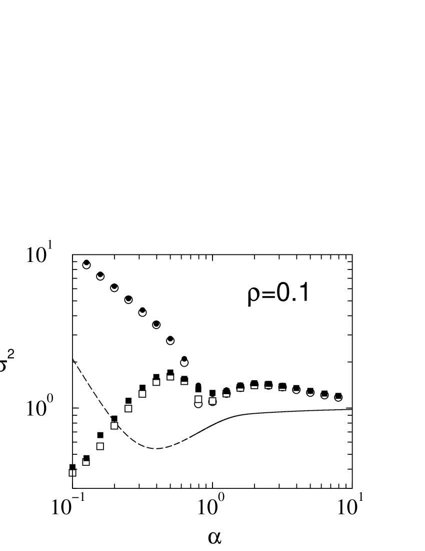
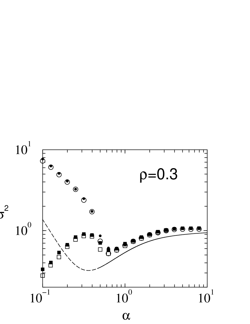
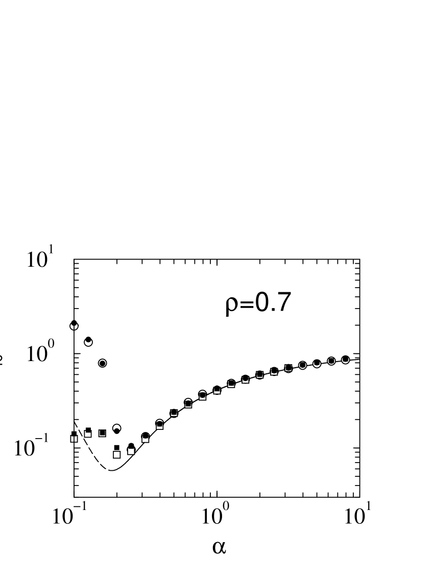
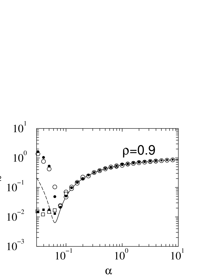
Figure 1: Volatility as a function of $\alpha$ for different values of $\rho$ for the batch game ($\rho_{i}=\rho\,\forall i$). Open symbols are from simulations of the batch process with $N=1000$ agents, averaged over $10$ samples of the disorder, and run for $500$ batch time steps. Filled markers are results from a direct iteration of the single-particle problem using the method of EissOppe92 ($5\times 10^{4}$ realisations of the single-agent process are generated, and the iteration is performed for $100$ time steps). Circles: tabula rasa start ($q_{i}(0)=0$), squares: biased starts ($|q_{i}(0)|=1$). Solid lines are the approximation of (34) for the ergodic phase and are continued as dashed lines into the non-ergodic phase (where the ergodic theory is longer valid).

3.2 Persistent order parameters in the ergodic stationary state

In order to analyse the ergodic state in the regime of large $\alpha$ we will make the following assumptions: (i) the system becomes stationary in the long-time limit, i.e. we will assume temporal translation invariance, $\lim_{t\to\infty}C_{t+\tau,t}=C(\tau)$ and $\lim_{t\to\infty}G_{t+\tau,t}=G(\tau)$, (ii) the absence of anomalous response, i.e. we will assume that the integrated response $\chi=\lim_{t\to\infty}\sum_{\tau\leq t}G(\tau)$ remains finite and (iii) weak long-term memory, i.e. $\lim_{t\to\infty}G_{tt^{\prime}}=0$ for all finite $t^{\prime}$.

The integrated response $\chi$ along with the persistent part of the correlation function, $c=\lim_{t\to\infty}t^{-1}\sum_{\tau\leq t}C(\tau)$, will be the order parameters characterising the ergodic stationary states of the game. The further analysis hence proceeds by formulating closed equations for these persistent order parameters.

Following HeimCool01 we introduce the re-scaled quantity $\tilde{q}_{\rho}(t)=q_{\rho}(t)/t$, and find from (13)

$$\tilde{q}_{\rho}(t) = \frac{1}{t}q_{\rho}(0)-\frac{1-\rho}{1-\overline{\rho}}\frac{\alpha}{t}\sum_{t^{\prime}<t}\sum_{t^{\prime\prime}}({\rm 1\!I}+G)^{-1}_{t^{\prime}t^{\prime\prime}}s_{\rho}(t^{\prime\prime})$$ (18)

$$+\theta_{\rho}+\frac{\sqrt{\alpha}}{t}\sqrt{\frac{1-\rho}{1-\bar{\rho}}}\sum_{t^{\prime}<t}\eta_{\rho}(t^{\prime})$$

Here, we have assumed that $\theta_{\rho}(t)=\theta_{\rho}$ for all $t$, so that $\theta_{\rho}$ is a static perturbation. Now, upon taking the limit $t\to\infty$ and writing $\tilde{q}_{\rho}=\lim_{t\to\infty}\tilde{q}_{\rho}(t)$, we find

$$\tilde{q}_{\rho}=-\alpha\frac{1-\rho}{1-\overline{\rho}}\frac{s_{\rho}}{1+\chi}+\theta_{\rho}+\sqrt{\alpha\frac{1-\rho}{1-\overline{\rho}}}\eta_{\rho},$$ (19)

where $s_{\rho}=\lim_{t\to\infty}t^{-1}\sum_{\tau\leq t}{\rm sgn}[q_{\rho}(\tau)]$ and
$\eta_{\rho}=\lim_{t\to\infty}t^{-1}\sum_{\tau\leq t}\eta_{\rho}(\tau)$. Note that $\tilde{q}_{\rho},s_{\rho}$ and $\eta_{\rho}$ are random variables, coupled through Eq. (19) with each realization corresponding to a realization of the single agent process (13). The variance of the zero-average Gaussian variable $\eta_{\rho}$ can be obtained from (14) and reads

$$\left\langle\eta_{\rho}^{2}\right\rangle_{\eta_{\rho}} = \lim_{\tau,\tau^{\prime}\to\infty}\frac{1}{\tau\tau^{\prime}}\sum_{t\leq\tau}\sum_{t^{\prime}\leq\tau^{\prime}}[({\rm 1\!I}+G)^{-1}D({\rm 1\!I}+G^{T})^{-1}]_{tt^{\prime}}$$ (20)

$$= \frac{\frac{\overline{\rho}}{1-\overline{\rho}}+c}{(1+\chi)^{2}}.$$

The analysis now proceeds along the lines of HeimCool01 , and we distinguish between so-called ‘frozen’ and ‘fickle’ agents. The distinction between frozen and fickle agents was first introduced in ChalMars99 and is based on observations from numerical simulations of batch and on-line MGs. One finds that some of the trajectories $q_{i}(t)$ of the original dynamics grow linearly in time in the stationary state, $q_{i}(t)\sim t$, so that the corresponding (frozen) agent always employs the same strategy. Other (fickle) agents keep switching strategies, and their score difference remains finite. While the distinction between frozen and fickle agents was originally made on the level of the initial $N$-particle dynamics, the same type of trajectories are also found in the realizations of the effective single particle process (generated for example using the method of EissOppe92 ). Frozen effective agents can be identified as those realizations of (13) for which $\tilde{q}_{\rho}\neq 0$. One then has $s_{\rho}={\rm sgn}[\tilde{q}_{\rho}]$. Using Eq. (19) (setting $\theta_{\rho}=0$) this is seen to be the case if $|\eta_{\rho}|>\gamma_{\rho}$, where $\gamma_{\rho}=\sqrt{\frac{\alpha(1-\rho)}{1-\overline{\rho}}}\frac{1}{1+\chi}$. On the other hand, a given realization of the representative agent process is ‘fickle’ when the score-difference $q_{\rho}(t)$ fluctuates around a finite value, with occasional zero-crossings, then one has $\tilde{q}_{\rho}=0$. This is the case if $|\eta_{\rho}|<\gamma_{\rho}$, and then $s_{\rho}=\eta_{\rho}/\gamma_{\rho}$. Note in particular that for fickle (effective) agents $s_{\rho}$ is a continuous variable, $-1<s_{\rho}<1$, with a non-zero value indicating that the corresponding effective agent employs his or her strategies with different frequencies.

From this the fraction of frozen agents with strategy correlation $\rho$ can be computed by performing the Gaussian integral over $\eta_{\rho}$ (with variance given by (20)):

$$\phi(\rho) = \left\langle\theta(|\eta_{\rho}|-\gamma_{\rho})|\rho\right\rangle_{\eta_{\rho}}$$ (21)

$$= 1-{\rm erf}\left(\frac{\lambda(\rho)}{\sqrt{2}}\right),$$

where we have introduced

$$\lambda(\rho)=\sqrt{\frac{\alpha(1-\rho)}{\overline{\rho}+(1-\overline{\rho})c}}.$$ (22)

$\theta$ in (21) is the step function; $\theta(x)=1$ if $x>0$, and $\theta(x)=0$ otherwise. The corresponding persistent part of the correlation function reads

$$c(\rho) \equiv \lim_{t\to\infty}t^{-1}\sum_{\tau\leq t}C_{\rho}(\tau)$$ (23)

$$= \left\langle s_{\rho}^{2}\right\rangle_{\eta_{\rho}}$$

$$= \left\langle\theta(|\eta_{\rho}|-\gamma)\right\rangle_{\eta_{\rho}}+\left\langle(\eta_{\rho}/\gamma_{\rho})^{2}\theta(\gamma_{\rho}-|\eta_{\rho}|)\right\rangle_{\eta_{\rho}}$$

$$= \phi(\rho)+\frac{1-\phi(\rho)}{\lambda(\rho)^{2}}-\frac{1}{\lambda(\rho)}\sqrt{\frac{2}{\pi}}\exp\left(-\lambda(\rho)^{2}/2\right).$$

Applying a static perturbation $\theta_{\rho}$ in (19) is (up to a prefactor $\sqrt{\alpha(1-\rho)/(1-\overline{\rho})}$) identical to perturbing the static random variable $\eta_{\rho}$. Such perturbations applied in the stationary state affect only fickle agents, for which we have $s_{\rho}=\eta_{\rho}/\gamma_{\rho}$. The susceptibility $\chi(\rho)\equiv\sum_{\tau}G_{\rho}(\tau)=\frac{\partial}{\partial\theta_{\rho}}\left\langle s_{\rho}\right\rangle_{\eta_{\rho}}$ may therefore be written as

$$\chi(\rho) = \sqrt{\frac{(1-\overline{\rho})}{\alpha(1-\rho)}}\left\langle\frac{\partial s_{\rho}}{\partial\eta_{\rho}}\right\rangle_{\eta_{\rho}}$$ (24)

$$= \gamma_{\rho}^{-1}\sqrt{\frac{(1-\overline{\rho})}{\alpha(1-\rho)}}\left(1-\phi(\rho)\right).$$

From these equations the overall persistent correlation $c$ and susceptibility $\chi$ can be computed self-consistently as

$$c = \int d\rho P(\rho)\frac{1-\rho}{1-\overline{\rho}}c(\rho),$$ (25)

$$\chi = \int d\rho P(\rho)\frac{1-\rho}{1-\overline{\rho}}\chi(\rho).$$ (26)

To this end, note that inserting (21) and (22) into (23) allows one to express $c(\rho)$ in terms of $c$ (and the model parameters $\alpha$ and $\overline{\rho}$).

4 Unimodal distribution of strategy correlations

We will now first investigate the case of a unimodal distribution of strategy correlations, $P(\rho^{\prime})=\delta(\rho-\rho^{\prime})$, i.e. the case where all $\rho_{i}$ are equal, $\rho_{i}\equiv\rho$, with $0\leq\rho<1$.

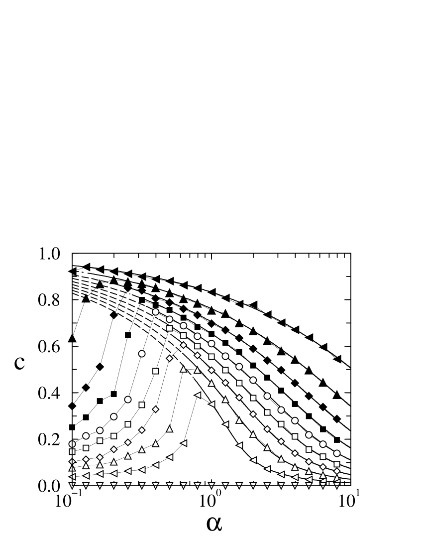
Figure 2: Persistent part $c$ of the correlation function for the batch game with $\rho_{i}=\rho$ for all $i$ and with tabula rasa initial conditions. Connected symbols are data obtained from simulations for $N=300$ players, measured over $500$ batch steps, preceded by an equilibration period of $500$ steps. The curves are $\rho=0.9,0.8,\dots,0$ from top to bottom. The solid lines are the theoretical predictions for the ergodic regime and have been continued as dashed lines by extrapolation of equations (27, 28) into the non-ergodic phase below $\alpha_{c}$, where they are no longer valid. The slight discrepancy between the theoretical lines and the numerical data close to the predicted breakdown of the ergodic theory is due to finite-size effects.

4.1 Stationary state in the ergodic regime and phase diagram

In this case the above self-consistent set of equations (25, 26) for the order parameters $c$ and $\chi$ can be compactified considerably using equations (22, 23, 24) and we find (with $c=c(\rho),\,\phi=\phi(\rho),\,\chi=\chi(\rho)$ and $\lambda=\lambda(\rho)$):

$$c = 1-\left(1-\frac{1}{\lambda^{2}}\right){\rm erf}\left(\frac{\lambda}{\sqrt{2}}\right)$$ (27)

$$-\frac{1}{\lambda}\sqrt{\frac{2}{\pi}}e^{-\lambda^{2}/2},$$

$$\chi^{-1} = \frac{\alpha}{{\rm erf}\left(\frac{\lambda}{\sqrt{2}}\right)}-1,$$ (28)

where

$$\lambda=\sqrt{\frac{\alpha}{\left(\frac{\rho}{1-\rho}+c\right)}}.$$ (29)

Note that $\overline{\rho}=\rho$ in the case of unimodal $P(\rho^{\prime})=\delta(\rho-\rho^{\prime})$. The fraction of frozen agents is given by $\phi=1-{\rm erf}(\lambda/\sqrt{2})$. Eqs. (27)-(28) agree with the corresponding equations for the static order parameters obtained within a replica symmetric theory ChalMarsZhan00 . They are easily solved numerically, and exact analytical predictions for $c,\phi$ and $\chi$ as functions of $\alpha$ can be obtained for $0\leq\rho<1$. Results for the persistent correlation $c$ are shown in Fig. 2, and we find very good agreement with numerical simulations for large $\alpha$, greater than critical values $\alpha_{c}(\rho)$. The deviations at lower values of $\alpha=P/N<\alpha_{c}(\rho)$ are due to a breakdown of the ergodic theory, more precisely of the assumption of finite integrated response HeimCool01 . The point $\alpha_{c}(\rho)$ at which this happens can be computed from Eq. (28). One finds that $\chi\to\infty$ at a critical value of $\alpha=\alpha_{c}(\rho)$ given by $\alpha_{c}(\rho)={\rm erf}(\lambda_{c}/\sqrt{2})$, where $\lambda_{c}=\lambda_{c}(\rho)$ fulfills

$${\rm erf}\left(\frac{\lambda_{c}(\rho)}{\sqrt{2}}\right)=1+\frac{\rho}{1-\rho}-\sqrt{\frac{2}{\pi}}\frac{1}{\lambda_{c}(\rho)}e^{-\lambda_{c}(\rho)^{2}/2}.$$ (30)

Solving this equation numerically leads to the phase diagram depicted in Fig. 3, with the critical line in the $(\alpha,\rho)$ plane separating the ergodic phase ($\chi$ finite) and the non-ergodic phase. This phase diagram for the MG with diversified strategies was first obtained from the corresponding replica calculation in ChalMarsZhan00 . While macroscopic observables such as the volatility are sensitive to the initial conditions in the non-ergodic phase, $\alpha<\alpha_{c}(\rho)$, the starting point is irrelevant in the ergodic phase, $\alpha>\alpha_{c}(\rho)$. We display the volatility for so-called tabula rasa starts ($q_{i}(0)=0$ for all $i$), and for randomly biased starts ($|q_{i}(0)|=q_{0}={\cal O}(1)$) in Fig. 1.

Figure 3: Phase diagram for the batch minority game with unimodal distribution of strategy correlations, $P(\rho^{\prime})=\delta(\rho^{\prime}-\rho)$.

4.2 Analytic approximations for the volatility

As we have seen it is possible to compute macroscopic order parameters of the stationary state, such as the fraction of frozen agents or the persistent part of the correlation function, exactly and in good agreement with simulations in the ergodic regime for general values of $\rho$. We will now turn to the magnitude of the market fluctuations $\sigma^{2}$. By performing a direct average in the generating functional, it was shown in HeimCool01 that the disorder-averaged volatility matrix $\overline{\Xi}$ is proportional to the correlator of the single-particle noise in the effective agent process. Generalizing the results of HeimCool01 to arbitrary values of $\rho$ we find the following exact result:

$$\overline{\Xi}_{tt^{\prime}}=(1-\rho)\Lambda_{tt^{\prime}}=(1-\rho)\left[({\rm 1\!I}+G)^{-1}D({\rm 1\!I}+G^{T})^{-1}\right]_{tt^{\prime}}.$$ (31)

Thus, an exact calculation of the volatility requires the computation of this matrix convolution, and hence the knowledge of both the long-term and transient behaviours of the dynamical order parameters $G(\tau)$ and $C(\tau)$ in the stationary state. To this end a full computation of the time-translation invariant solutions of the self-consistent representative agent problem would be necessary. Due to the retarded self-interaction and the presence of the coloured single-particle noise, this is in general impossible. One therefore has to resort to approximations, and the generally accepted approach first presented in HeimCool01 aims at expressing the market volatility in terms of the persistent order parameters $c,\phi$ and $\chi$.

To this end one separates the contribution of the frozen agents to the correlation function $C$ from the contribution of the fickle agents and writes

$$C(t-t^{\prime})=\phi+(1-\phi)\left\langle s_{\rho}(t)s_{\rho}(t^{\prime})\right\rangle_{fi},$$ (32)

where the average $\left\langle\dots\right\rangle_{fi}$ extends only over fickle agents. Inserting this into (31) and recalling
$\sigma^{2}=\lim_{T\to\infty}T^{-1}\sum_{t\leq T}\overline{\Xi}_{tt}$ leads to

$$\frac{1}{1-\rho}\sigma^{2} = \frac{\frac{\rho}{1-\rho}+\phi}{(1+\chi)^{2}}+(1-\phi)$$ (33)

$$\times\lim_{\tau\to\infty}\tau^{-1}\sum_{t\leq\tau}\left\langle\left[\sum_{t^{\prime}\leq t}({\rm 1\!I}+G)^{-1}_{tt^{\prime}}s_{\rho}(t^{\prime})\right]^{2}\right\rangle_{fi}.$$

In HeimCool01 , for $\rho=1/2$, the authors proceeded by keeping only the instantaneous contribution, $t=t^{\prime}$, in the last term. Generalizing their calculation to arbitrary $0\leq\rho<1$ one obtains the following approximate expression

$$\sigma^{2}=(1-\rho)\left[\frac{\rho/(1-\rho)+\phi}{(1+\chi)^{2}}+(1-\phi)\right].$$ (34)

Fig. 1 demonstrates that this approximation is in good agreement with data from simulations of the original batch process for $\rho\gtrsim 1/2$, but that it becomes less accurate as $\rho$ is reduced. In particular we note that in simulations we find volatilities $\sigma^{2}>1$ in the ergodic phase of batch games with largely anti-correlated strategies, i.e. low values of $\rho$, while (34) predicts a volatility below the random trading limit $\sigma^{2}=1$ for all values of $\rho$ and $\alpha\geq\alpha_{c}(\rho)$. We have verified explicitly that the discrepancy between this analytical approximation and the numerically measured volatility can be traced back to the omission of the non-instantaneous terms in (33): iterating the single-particle process using the Eissfeller-Opper algorithm EissOppe92 , measuring the contributions from the frozen and fickle agents, respectively, and taking into account all terms of (33) restores the agreement with direct numerical simulations of the batch process. The discrepancy between the approximation of Eq. (34) and the volatility measured in simulations becomes extremal in the fully anti-correlated case. In this case one finds no frozen agents, and inserting $\rho=0$ and $\phi=0$ into (34) gives $\sigma^{2}=1$ for $\alpha>\alpha_{c}(\rho=0)=1$. In numerical simulations of the batch process, however, we find a decreasing relation $\sigma^{2}=\sigma^{2}(\alpha)$, and $\sigma^{2}=1$ is only approached in the limit $\alpha\to\infty$, see Fig. 4. In the next section, we will study the case of fully anti-correlated strategies in more detail, and will derive different analytical approximations for the global market fluctuations in this case.

4.3 The fully anti-correlated case

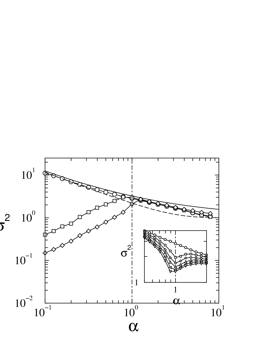
Figure 4: Volatility as a function of $\alpha$ for $\rho=0$ for the batch game. Connected symbols are from simulations started from different initial conditions (circles are tabula rasa starts, $|q_{i}(0)|=0$, squares are $|q_{i}(0)|=2.0$ and diamonds $|q_{i}(0)|=10.0$). The solid and dashed lines are the approximations of Eqs. (41) and (42) respectively. The vertical dot-dashed line marks the analytically predicted location of the phase transition at $\alpha_{c}(\rho=0)=1$. Inset: $\sigma^{2}$ vs $\alpha$ for $\rho=0.0,0.01,0.02,0.03,0.04,0.05$ from top to bottom (tabula rasa starts).

In the special case of completely anti-correlated strategies, $\rho=0$, and tabula rasa starts, we observe experimentally that the system is always in a fully oscillating phase, i.e. that all agents switch strategies at each time step, and that accordingly $C(\tau)=(-1)^{\tau}$ for all $\tau$. Eq. (27) for $\rho=0$ is indeed solved by $c=0$ so that no frozen agents are possible. We will use this observation as an ansatz, which will allow us to proceed analytically and to give an approximate expression for the volatility, which is different from the one (derived for general $\rho$) in the previous section. Its derivation is similar to the analysis of the non-ergodic state in the limit $\alpha\to 0$ of the standard batch MG HeimCool01 . In this limit of the game with uncorrelated strategies a similar oscillatory state is found.

For $\rho=0$, we have $D(\tau)=C(\tau)=(-1)^{\tau}$ and using Eq. (31), we conclude that the correlation matrix of the single-particle noise in the stationary state is given by $\Lambda_{tt^{\prime}}=(-1)^{t-t^{\prime}}\Upsilon^{2},$ where $\Upsilon=\sum_{\tau}(-1)^{\tau}({\rm 1\!I}+G)^{-1}(\tau)$. Thus, for any fixed realization of the single-particle noise $\eta_{0}(t)$ must be of the form $\eta_{0}(t)=\Upsilon z(-1)^{t}$, where $z$ is a (static) Gaussian random variable of zero mean and unit variance (note that the subscript in $\eta_{0}(t)$ indicates that we are concerned with the case $\rho=0$ in this section, similarly for $q_{0}(t)$ and $\tilde{s}_{0}$ below). A given stochastic value of $z$ determines the oscillation amplitude and sign of the corresponding trajectory of the noise $\eta_{0}(t)$. The volatility in this fully oscillatory state can be obtained as $\sigma^{2}=\lim_{T\to\infty}T^{-1}\sum_{t\leq T}\Lambda_{tt}=\Upsilon^{2}$, so that it remains to compute $\Upsilon$. Upon introduction of

$$\tilde{s}_{0}\equiv\lim_{\tau\to\infty}\tau^{-1}\sum_{t\leq\tau}(-1)^{t}{\rm sgn}[q_{0}(t)]$$ (35)

we can use the identity

$$\sqrt{\alpha}\sum_{t^{\prime\prime}}\left\langle\eta_{0}(t)\eta_{0}(t^{\prime\prime})\right\rangle_{\eta_{0}}G_{t^{\prime}t^{\prime\prime}}=\left\langle{\rm sgn}[q_{0}(t^{\prime})]\eta_{0}(t)\right\rangle_{\eta_{0}}$$ (36)

(obtained by an integration by parts in the generating functional HeimCool01 ) to write $\Upsilon$ as

$$\Upsilon=1-\frac{1}{\sqrt{\alpha}}\left\langle\tilde{s}_{0}z\right\rangle_{z},$$ (37)

where $\left\langle\dots\right\rangle_{z}$ denotes an average over the standard Gaussian variable $z$. We have also used the fact that $\sum_{\tau}(-1)^{\tau}({\rm 1\!I}+G)^{-1}(\tau)=[1+\sum_{\tau}(-1)^{\tau}G(\tau)]^{-1}$ here HeimCool01 .

In order to compute the average $\left\langle\tilde{s}_{0}z\right\rangle_{z}$, we note that from the effective single-agent process we can derive the relation

$$\widetilde{\Delta q_{0}}=-\alpha\Upsilon\tilde{s}_{0}+\sqrt{\alpha}\tilde{\eta}_{0}$$ (38)

between the staggered averages $\tilde{s}_{0}$ and

$$\widetilde{\Delta q_{0}} = \lim_{\tau\to\infty}\tau^{-1}\sum_{t\leq\tau}(-1)^{t}(q_{0}(t+1)-q_{0}(t)),$$ (39)

$$\tilde{\eta}_{0} = \lim_{\tau\to\infty}\tau^{-1}\sum_{t\leq\tau}(-1)^{t}\eta_{0}(t).$$ (40)

Since the effective agents are purely oscillatory, one has ${\rm sgn}(\widetilde{\Delta q_{0}})=-\tilde{s}_{0}$. Using Eq. (38) and the relation $\eta_{0}(t)=\Upsilon z(-1)^{t}$ we therefore require ${\rm sgn}[z]=-\tilde{s}_{0}$, i.e. $\tilde{s}_{0}z=-|z|$ for any given realization of $z$ with $\sqrt{\alpha}\Upsilon|z|>\alpha\Upsilon$ (and the corresponding realization of the effective agent process). Since $\Upsilon$ comes out positive this is the case for realizations with $|z|>\sqrt{\alpha}$. For $|z|<\sqrt{\alpha}$ both signs $\tilde{s}_{0}z=\pm|z|$ are possible; using the Eissfeller-Opper algorithm we have checked that indeed both signs are taken in this case. A similar complication has been encountered in the context of mixed Minority/Majority Games in DeMaGiarMose03 .

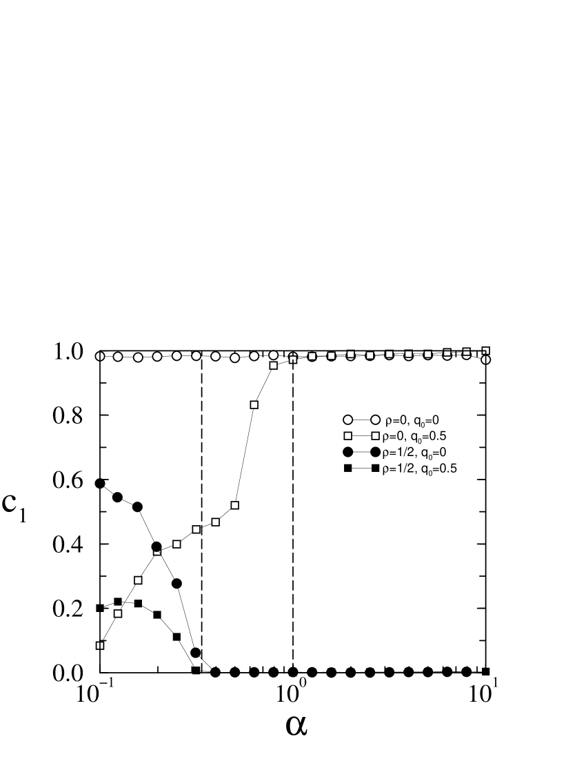
Figure 5: Amplitude of oscillations of the correlation function as a function of $\alpha$ for the batch game for $\rho=1/2$ (filled markers) and $\rho=0$ (open markers). Results are from simulations with $N=500$ agents, run for $500$ batch steps and averaged over $10$ realisations of the disorder. In the simulations we measure $c_{1}$ in the stationary state as $c_{1}=(2T)^{-1}\sum_{\tau=T}^{2T}|C(\tau+1)-C(\tau)|$, where $T=125$ batch steps. Circles are data for tabula rasa starts, squares from simulations with biased starts ($q_{0}=0.5$). The vertical dashed lines mark the locations of the phase transition of the games with uncorrelated strategies at $\alpha_{c}(\rho=1/2)\approx 0.3374$ and at $\alpha_{c}(\rho=0)=1$ for fully anticorrelated strategies.

We have two possibilities to proceed: firstly, we can assume that $\tilde{s}_{0}z=-|z|$ also for $-\sqrt{\alpha}<z<\sqrt{\alpha}$, and that deviations from this behaviour will only have a small effect on the volatility. We then end up with the following approximation

$$\sigma^{2} \approx \left(1+\frac{1}{\sqrt{\alpha}}\left\langle|z|\right\rangle_{z}\right)^{2}$$ (41)

$$= \left(1+\sqrt{\frac{2}{\pi\alpha}}\right)^{2}.$$

Alternatively, we can assume that both signs $\tilde{s}_{0}z=\pm|z|$ are taken equally often for $|z|<\sqrt{\alpha}$ so that this interval does not contribute to the average $\left\langle\tilde{s}_{o}z\right\rangle_{z}$. We then find

$$\sigma^{2} \approx \left(1+\sqrt{\frac{2}{\pi\alpha}}e^{-\alpha/2}\right)^{2}.$$ (42)

As depicted in the main panel of Fig. 4 the approximations of (41) and (42) appear to form upper and lower bounds of the volatility, respectively. Both approximations become exact only in the limit $\alpha\to 0$, but reproduce the behaviour of $\sigma^{2}=\sigma^{2}(\alpha)$ quite well, even for larger values of $\alpha\approx 1$.

We conclude this section by mentioning that the batch MG with fully anti-correlated strategies, $\rho=0$, is different from the cases $0<\rho<1$ in two respects: (i) the fully anti-correlated case exhibits oscillatory behaviour, $C(\tau)=(-1)^{\tau}$, for all $\alpha$, even above $\alpha_{c}(\rho=0)=1$, whereas in all other cases oscillations decay above $\alpha_{c}$ and persist only in the non-ergodic phase, where one finds correlation functions of the form $C(\tau)=c_{0}+c_{1}(-1)^{\tau}$ for $\tau>0$. This is illustrated in Fig. 5, where we plot $c_{1}$ as a function of $\alpha$ for different values of $\rho$; (ii) the volatility plotted as a function of $\alpha$ exhibits a minimum at $\alpha_{c}(\rho)$ for all $0<\rho<1$, but is decreasing monotonically for $\rho=0$, see the inset of Fig. 4. Nevertheless the stationary volatility in the fully anti-correlated case does depend on initial conditions below $\alpha_{c}(\rho=0)=1$, whereas the starting point is irrelevant for $\alpha>1$.

4.4 Comparison with the on-line game

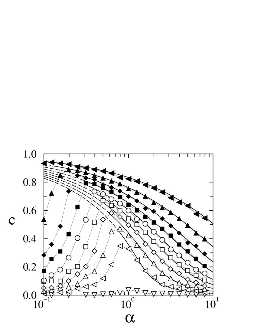
Figure 6: Persistent part $c$ of the correlation function for the on-line game with $\rho_{i}=\rho$ for all $i$ and with tabula rasa initial conditions. Connected symbols are data obtained from simulations for $N=300$ players, measured over $25000$ on-line steps, preceded by an equilibration period of $25000$ steps. The curves are $\rho=0.9,0.8,\dots,0$ from top to bottom. The solid lines are the theoretical predictions for the ergodic regime and have been continued as dashed lines by extrapolation into the non-ergodic phase below $\alpha_{c}$, where they are no longer valid. The slight discrepancy between the theoretical lines and the numerical data close to the predicted breakdown of the ergodic theory is due to finite-size effects.

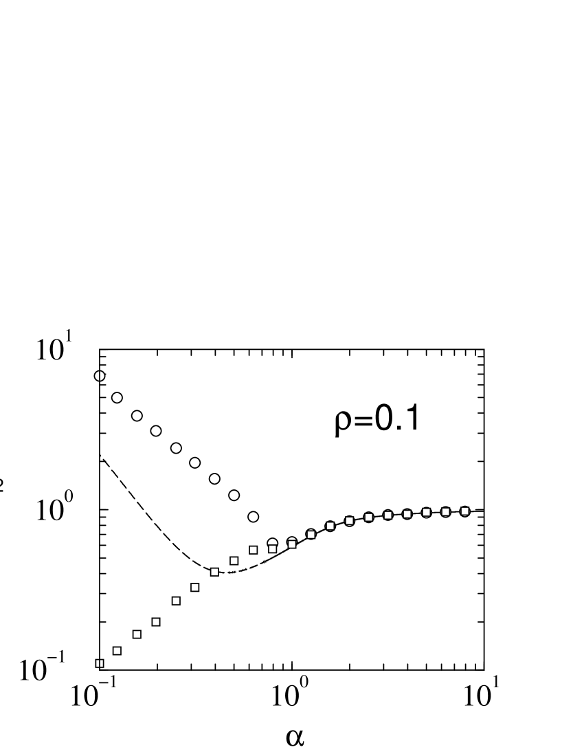
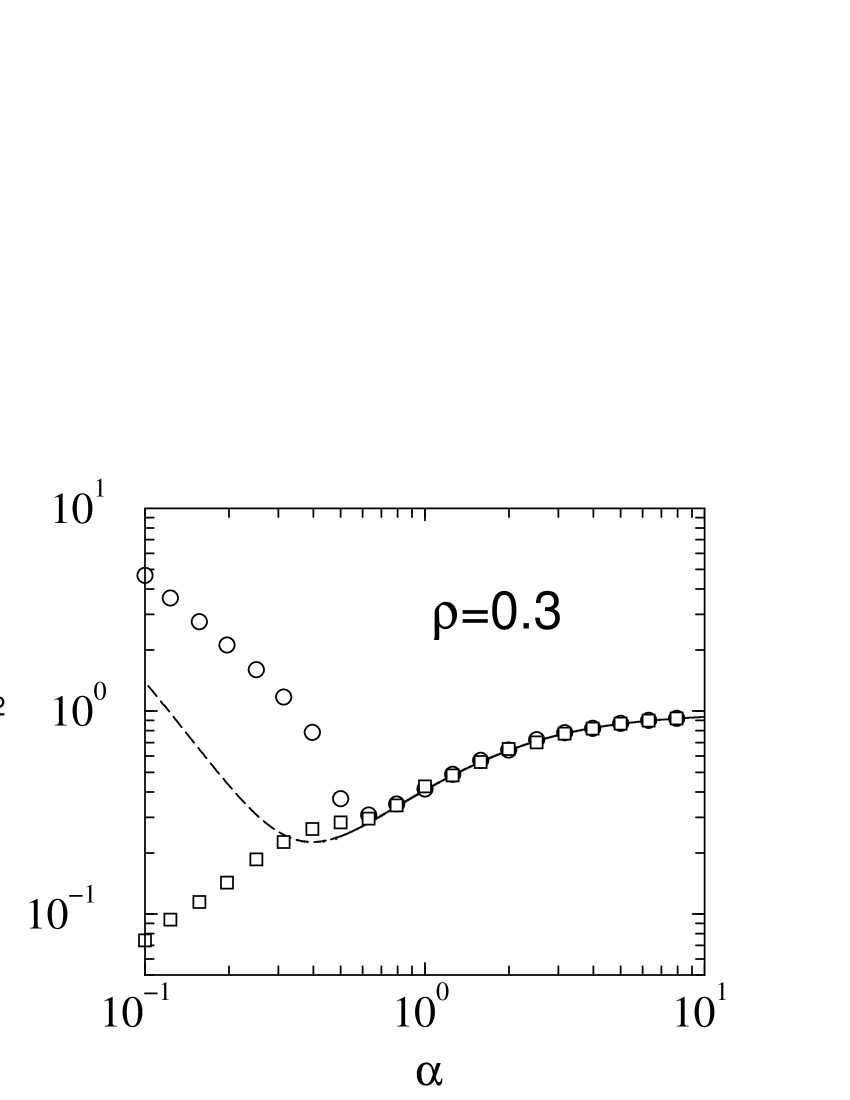
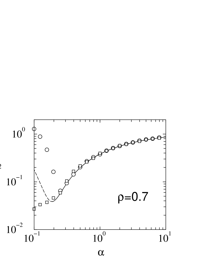
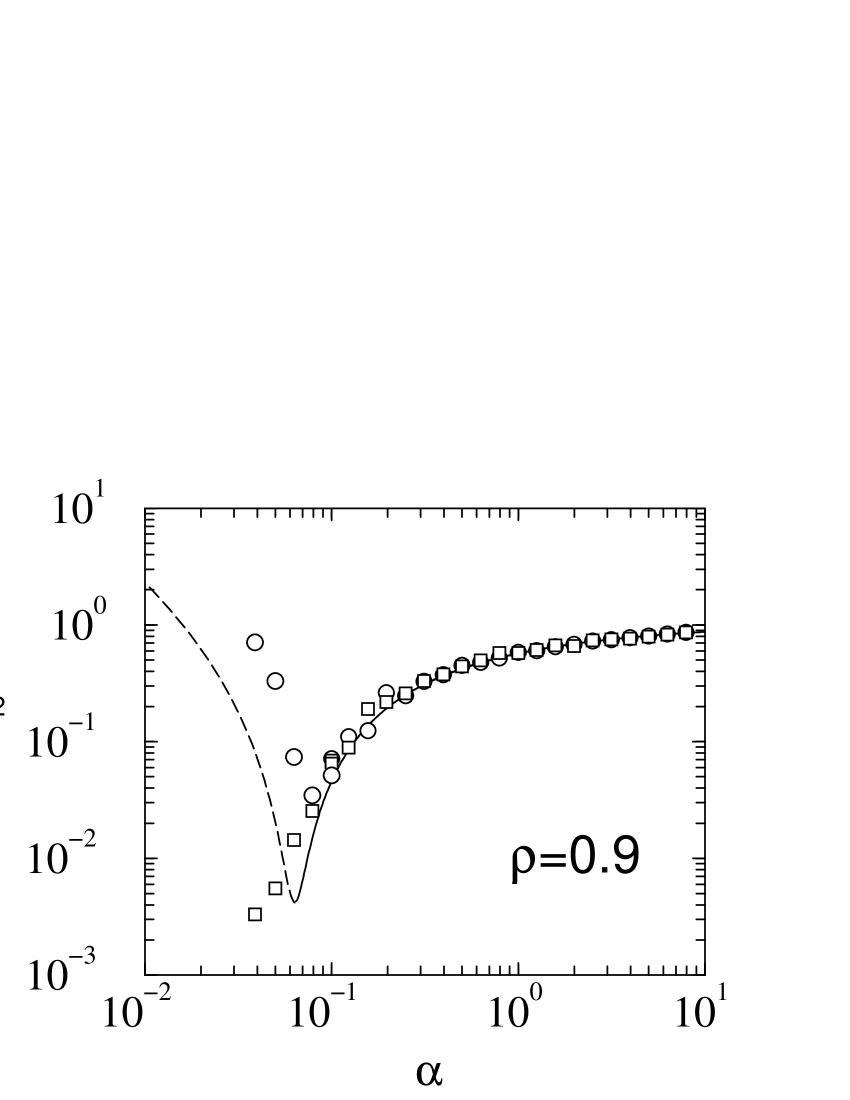
Figure 7: Volatility as a function of $\alpha$ for different values of $\rho$ for the on-line game ($\rho_{i}=\rho$ for all agents). Solid lines are the approximation of (44) for the ergodic phase and are continued as dashed lines into the non-ergodic phase (where the ergodic theory is no longer valid). Markers are from simulations of the on-line process with $N=300$ agents ($N=1000$ for $\rho=0.9$), averaged over $10$ samples of the disorder, and run for $10^{5}$ on-line time steps. Circles: tabula rasa start ($q_{i}(0)=0$), squares: biased starts ($|q_{i}(0)|=3$).

We will now turn to the case of on-line learning rules, and will discuss the influence of the timing of adaptation of the agents on the behaviour of MGs with correlated strategies.

A generating functional theory for the on-line game with random external information and uncorrelated strategies has been worked out in CoolHeim01 . The analysis has to deal with the explicit dependence on the external information, and inevitably requires a much more elaborate mathematical formalism than the analysis of the batch game. The resulting theory is easily adapted to the case of general strategy assignments with arbitrary correlations. We will not report the mathematical details of the calculation, but will only state that, in the ergodic regime, it leads to self-consistent equations for the persistent order parameters (such as $c,\phi$ and $\chi$), which are identical to the ones of the batch MG with general strategy correlations. As a consequence, the location of the phase transition (marked by an onset of diverging integrated response) is identical in batch and on-line games with the same distribution $P(\rho)$ of correlation parameters. Results for the persistent correlation $c$ as a function of $\alpha$ are compared with simulations of the on-line game with unimodular strategy correlations in Fig. 6. The on-line simulations shown in Fig. 6 essentially also match those of the batch case shown in Fig. 2 for the ergodic region.

Numerical simulations, however, reveal crucial differences between the volatilities of the on-line and batch games with correlated strategies. A comparison of Figs. 1 and 7 shows that in their ergodic states the volatility of batch games can take values both above and below the random trading limit $\sigma^{2}=1$ , whereas that in on-line games never exceeds $\sigma^{2}=1$. The difference between the volatilites of batch and on-line games becomes maximally pronounced in the fully anti-correlated case, compare Figs. 4 and 8. In the on-line game with $\rho=0$ we find that the volatility is equal to one for all $\alpha>\alpha_{c}(\rho=0)=1$, whereas it approaches this random trading limit only asymptotically for $\alpha\to\infty$ in the batch case. Allowing the agents to switch stategies only every $M$ time steps according to the update rule (2) one can interpolate between the batch and on-line cases: Fig. 9 shows the volatility $\sigma^{2}$ as a function of $\alpha$ for the fully anti-correlated case for different intermediate choices of $M$. While small values of $M\ll P$ produce market fluctuations close to those of the on-line game (which corresponds to $M=1$), the batch limit is obtained for $M\geq{\cal O}(P)$.

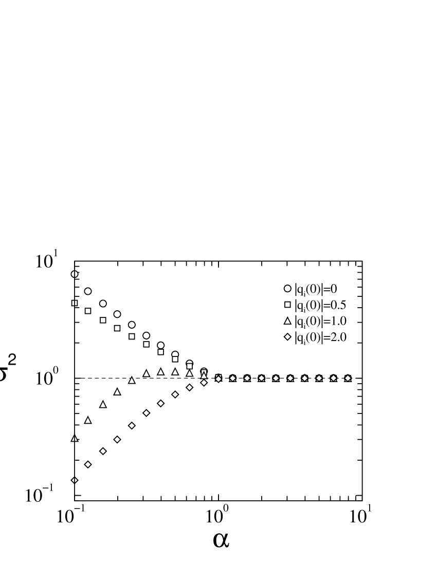
Figure 8: Volatility as a function of $\alpha$ for the on-line game at $\rho=0$, and for different values of the initial bias $|q_{i}(0)|$. All data is from simulations with $N=300$ agents averaged over $10$ samples of the disorder.

Similarly to the batch case, a computation of the transient parts of the dynamical order parameters would be necessary to obtain exact expressions for the volatility of on-line MGs. As this is in general not feasible, one proceeds as in the batch case, and tries to find approximate expressions in terms of the persistent order parameters only. Such an approach was first proposed for on-line games in CoolHeim01 , and is slightly different from the approximations in the batch case. The approximation is based on the observation that in mean-field disordered systems with detailed balance fluctuation-dissipation relations can be used to ‘transform away’ non-persistent parts of the response and correlation functions without changing averages of single-time observables and averages of two-time quantities at infinite time-separations. For equilibrium systems with detailed balance this approach is exact Cool00b . It can be used to extract the static order parameters as obtained in a replica-symmetric equilibrium approach from the generating functional equations. Details of this procedure can be found in Cool00b ; HeimelThesis .

Although the MG does not exhibit detailed balance a similar ad-hoc procedure for removing the non-persistent parts of the order parameters has been successfully employed to obtain approximations for the volatility in CoolHeim01 . It amounts to assuming that $C$ and $G$ are of the following form:

$$C_{tt^{\prime}}=c+(1-c)\delta_{tt^{\prime}},~{}~{}~{}~{}~{}~{}~{}~{}~{}~{}~{}G_{tt^{\prime}}=\chi\delta(1-\delta)^{t-t^{\prime}-1}\,(\mbox{for }t>t^{\prime}),$$ (43)

with the limit $\delta\to 0$ to be taken at the end of the calculation. In this way one preserves
$\lim_{\tau\to\infty}C(\tau)=c$ and $\sum_{\tau}G(\tau)=\chi$, but removes non-persistent contributions.

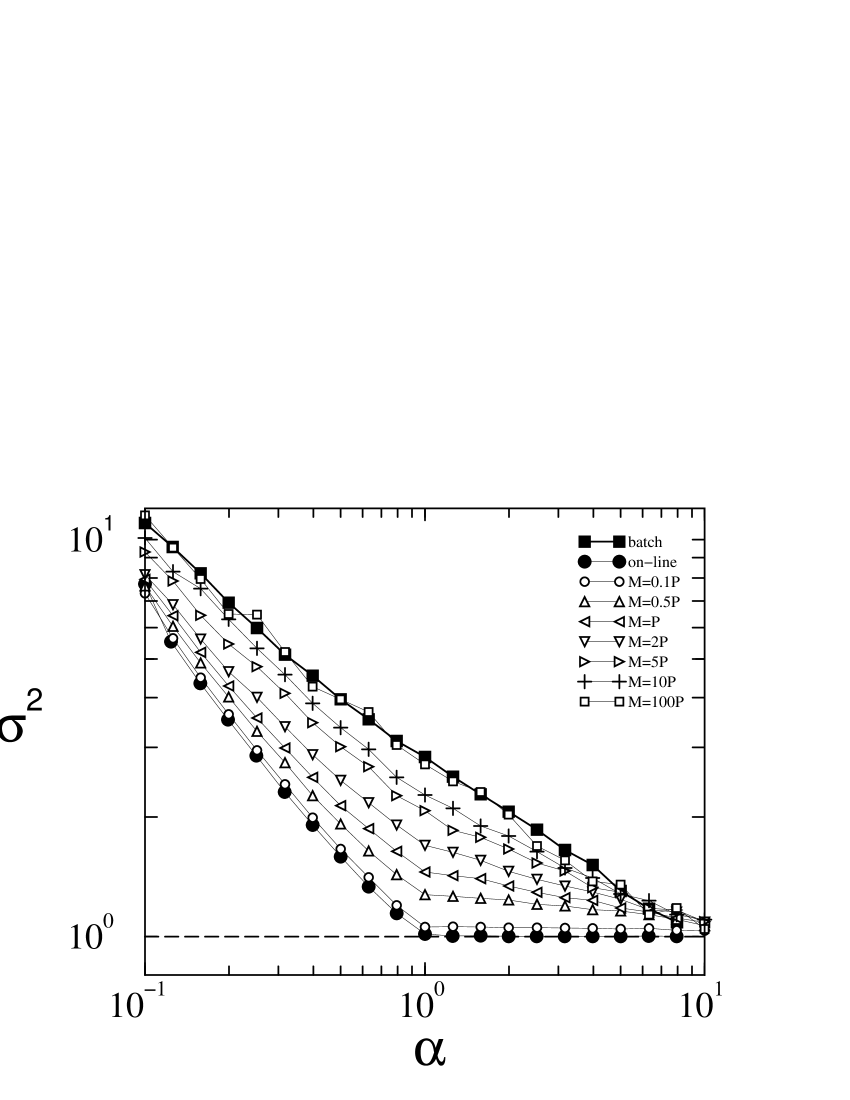
Figure 9: Volatility of a MG with fully anti-correlated strategies ($\rho_{i}=0$ for all $i$) and in which switching of strategies is allowed only every $M$ time steps. The individual curves are for different values of $M$. All data is from simulations performed at a constant number $P=\alpha N=50$ of possible states of the external information $\mu$ and were run for $10^{6}$ on-line steps. Results are averages over $20$ realisations of the disorder. The corresponding curves for the on-line and batch games are displayed as filled symbols for comparison. The lines connecting the markers are guides to the eye.

This approach is easily generalised to the case of unimodular distributions of the correlation parameter, and upon making the standard assumptions on time-translation invariance and ergodicity, one obtains the following approximate expression for the volatility

$$\sigma^{2}=(1-\rho)\left[\frac{\rho/(1-\rho)+c}{(1+\chi)^{2}}+(1-c)\right],$$ (44)

which differs only slightly from the approximate result for the batch game, Eq. (34). As shown in Fig. 7 this approximation is accurate in the ergodic phase for all values of $\rho$, even in a regime where the corresponding approximation for the batch MG is not satisfactory to describe the volatility measured in numerical experiments. We attribute the deviations slightly above the transition to finite-size effects. Applying the same method to the volatility of the batch game also leads to Eq. (44) and hence to the same qualitative and quantative discrepancy between the numerically measured and analytically estimated volatilities in batch games with largely anti-correlated strategies. See also MGbook2 for alternative derivations of Eq. (44) for batch and on-line games with uncorrelated strategies.

Eq. (44) agrees with the approximation for the volatility derived from the replica analysis of the MG with diversified strategies ChalMarsZhan00 . We note that the analogue of the removal of the non-persistent parts of $C$ and $G$ in the dynamical approach is reflected by an assumption on the cross-correlations between the agents in the replica formalism of ChalMarsZhan00 . Based on the assumption that $\left\langle s_{i}s_{j}\right\rangle=\left\langle s_{i}\right\rangle\left\langle s_{j}\right\rangle$ for $i\neq j$ the authors of ChalMarsZhan00 neglect a term $\Delta\equiv N^{-1}\sum_{i\neq j}\sum_{\mu}\xi_{i}^{\mu}\xi_{j}^{\mu}(\left\langle s_{i}s_{j}\right\rangle-\left\langle s_{i}\right\rangle\left\langle s_{j}\right\rangle)$, in the ergodic phase ($\alpha>\alpha_{c}$). Here again $s_{i}(t)={\rm sgn}[q_{i}(t)]$, and $\left\langle\dots\right\rangle$ denotes an average over time. While our findings concerning the volatility suggest that this assumption is appropriate in the on-line game, it appears to be inaccurate in the batch game at low values of $\rho$. We have confirmed this numerically in simulations of the batch MG. At fixed $\alpha>1$ we find that $\Delta=\Delta(\alpha,\rho)$ is close to zero for large values of $\rho\simeq 1$, but increases as $\rho$ approaches zero. While we do not depict these results here, we will only point out that for $\rho=0$ we find oscillatory behaviour, $s_{i}(t)=s_{i}(0)(-1)^{t}$, at all $\alpha$, so that $\left\langle s_{i}\right\rangle=0$, but $\left\langle s_{i}s_{j}\right\rangle=\pm 1$. One then has $\left\langle s_{i}s_{j}\right\rangle-\left\langle s_{i}\right\rangle\left\langle s_{j}\right\rangle=\pm 1\neq 0$ so that the above approximation fails.

To conclude the discussion of the volatility in on-line models, we would like to mention that the volatility of MGs with real histories and fully anti-correlated strategies behaves qualitatively like the one of the on-line MG with random history, with $\sigma^{2}=1$ for $\alpha>1$ ChalletThesis .

Finally, in this section, let us briefly address the role of global oscillations in on-line MGs. As an analytical treatment of this dynamical feature would require a solution of the transient behaviour of the dynamical order parameters (which is still awaited) the results in the remainder of this section and in section 4.5 are all based on direct numerical simulations of the games under consideration. Anti-persistent behaviour in the on-line MG with uncorrelated strategies and with real market histories was identified first in ChalMars99 , where the authors find oscillatory behaviour below $\alpha_{c}$, but no persistent oscillations in the high-$\alpha$ phase, in qualitative agreement with results for batch games HeimCool01 , recall also Fig. 5. In ChalMars99 the authors considered an on-line version of the MG in which the agents use only the sign of the total bid to update their strategy scores, i.e. a model, in which $A(\ell^{\prime})$ in Eq. (1) is replaced by $\pi(\ell^{\prime})={\rm sgn}[A(\ell^{\prime})]$. We will refer to this as the ‘sign-update’ rule, as opposed to the linear relation (1). The authors then consider a conditional correlation function

$$C_{\pi\pi}(\tau)=P^{-1}\sum_{\mu=1}^{P}\left\langle\pi(\ell)\pi(\ell+\tau)|\mu\right\rangle$$ (45)

in the stationary state, where the average $\left\langle\pi(\ell)\pi(\ell+\tau)|\mu\right\rangle$ extends only over times $\ell$ and $\ell+\tau$ for which $\mu(\ell)=\mu(\ell+\tau)=\mu$. Similarly we can define a conditional ‘spin-spin’ correlation function according to

$$C_{ss}(\tau)=(NP)^{-1}\sum_{\mu=1}^{P}\sum_{i=1}^{N}\left\langle s_{i}(\ell)s_{i}(\ell+\tau)|\mu\right\rangle.$$ (46)

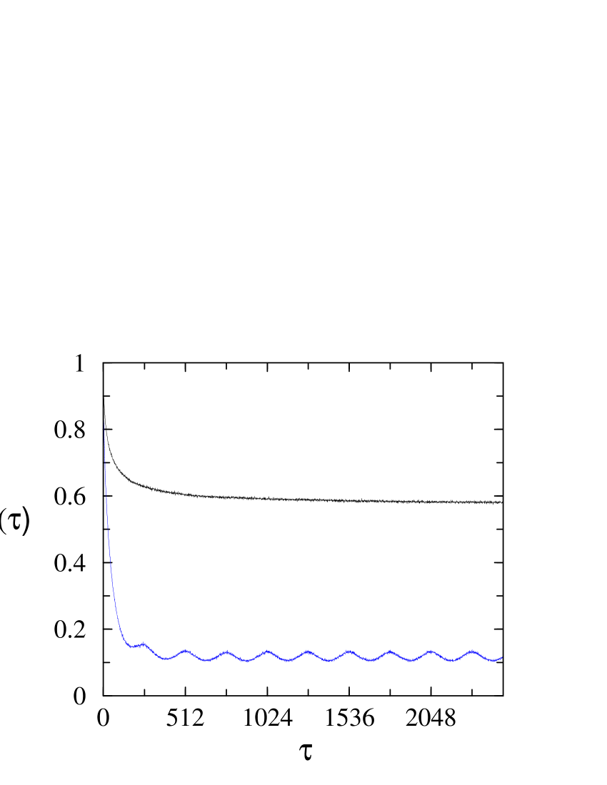
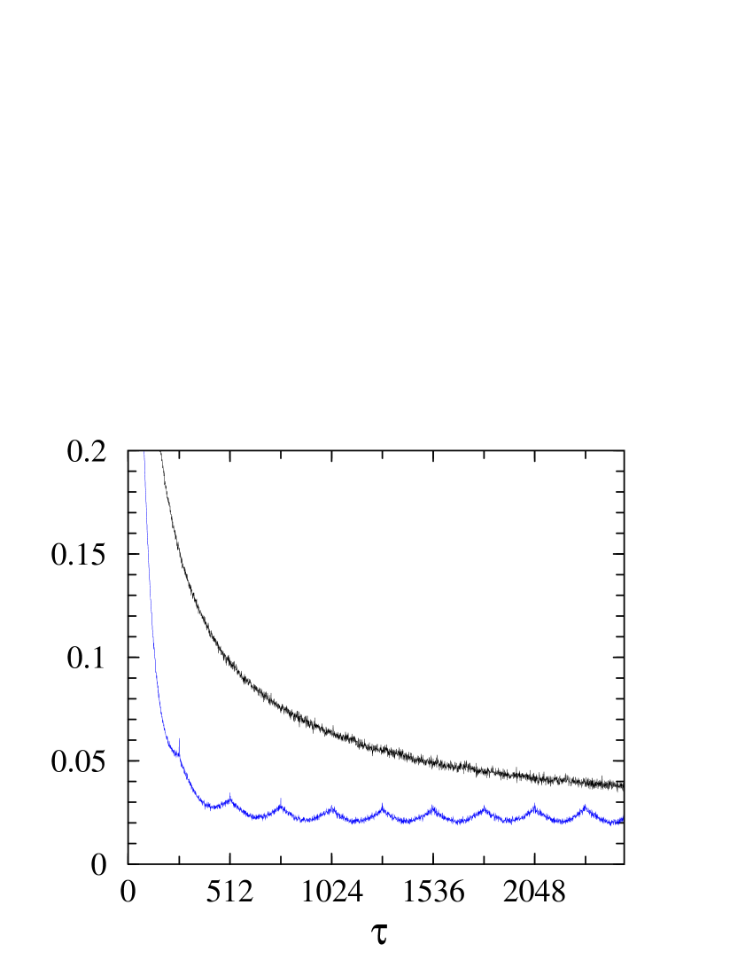
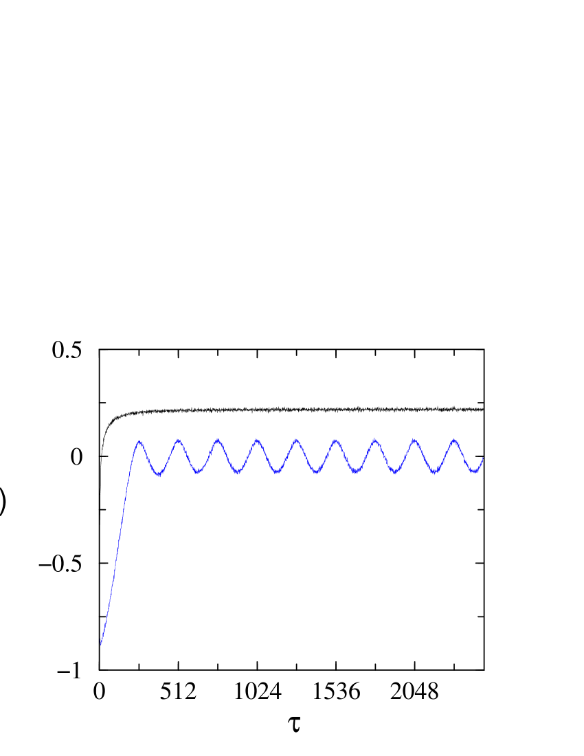
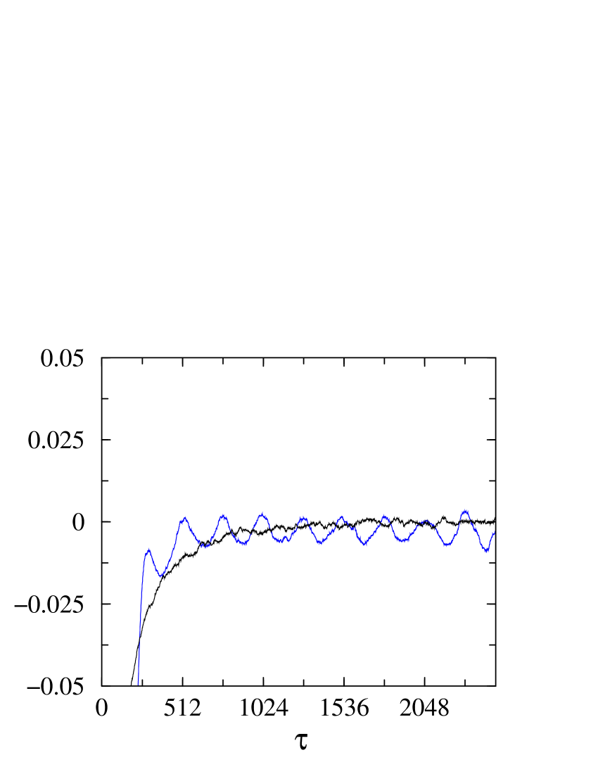
Figure 10: Correlation functions for the on-line game with real market histories. All data are from simulations at $P=\alpha N=128$, run for $10^{5}$ on-line time steps. Left column: $\rho=0.5$, the oscillatory curves are at $\alpha=0.1$, below the transition, non-oscillatory curves at $\alpha=1.25$, above the transition. Right column: $\rho=0.0$, oscillatory curves $\alpha=0.1$, non-oscillatory curves $\alpha=1.58$. The upper two panels show the ‘spin-spin’ correlation function, $C_{ss}(\tau),$ conditional on the information pattern, the lower two panels the conditional correlation function, $C_{\pi\pi}(\tau)$, of the sign of the total bid $\pi(\ell)={\rm sgn}[A(\ell)]$ (see text for further explanantions). Averages over $10$ to $100$ realisations of the disorder are taken. Results for $C_{\pi\pi}$ at $\rho=0$ are displayed as running averages over $64$ points to smoothen the noisy raw data.

Fig. 10 demonstrates that the games both with uncorrelated strategies ($\rho=1/2$), and with anti-correlated strategies ($\rho=0$), respectively, show anti-persistence in their non-ergodic states, $\alpha<\alpha_{c}(\rho)$, but not above $\alpha_{c}$: $C_{\pi\pi}$ and $C_{ss}$ exhibit oscillations of period $2P$ below $\alpha_{c}$, but approach a constant value above the transition. In particular the behaviour of the on-line game with anti-correlated strategies appears crucially different from its batch counterpart in this respect: in the batch game with anti-correlated strategies we find oscillatory behaviour for all values of $\alpha$, whereas in the on-line case with real histories and sign-updates, they are found only in the low-$\alpha$ phase.

Before turning to the next section, we would like to remark that the oscillations below $\alpha_{c}$, first reported in ChalMars99 , are generally not detected very easily in on-line games: we have tested several other variations of the model and observables and found that no oscillatory behaviour can be observed if (i) the linear update (1) is used instead of the sign-update prescription, (ii) if unconditional correlation functions are considered instead of conditional ones or if (iii) real market histories are replaced by fake histories.

While no persistent oscillations are found in unconditional correlation functions of on-line games with random histories, oscillations emerge gradually for $\alpha<\alpha_{c}(\rho=0.5)$ in the case of uncorrelated strategies, and for all $\alpha$ in the anti-correlated case, as the time lag $M$ between two successive strategy updates is increased to approach the batch limit, see Fig. 11 (oscillation amplitude for on-line games is not shown, but is indistinguishable from zero on the scale of Fig. 11).

4.5 Random timing of adaptation

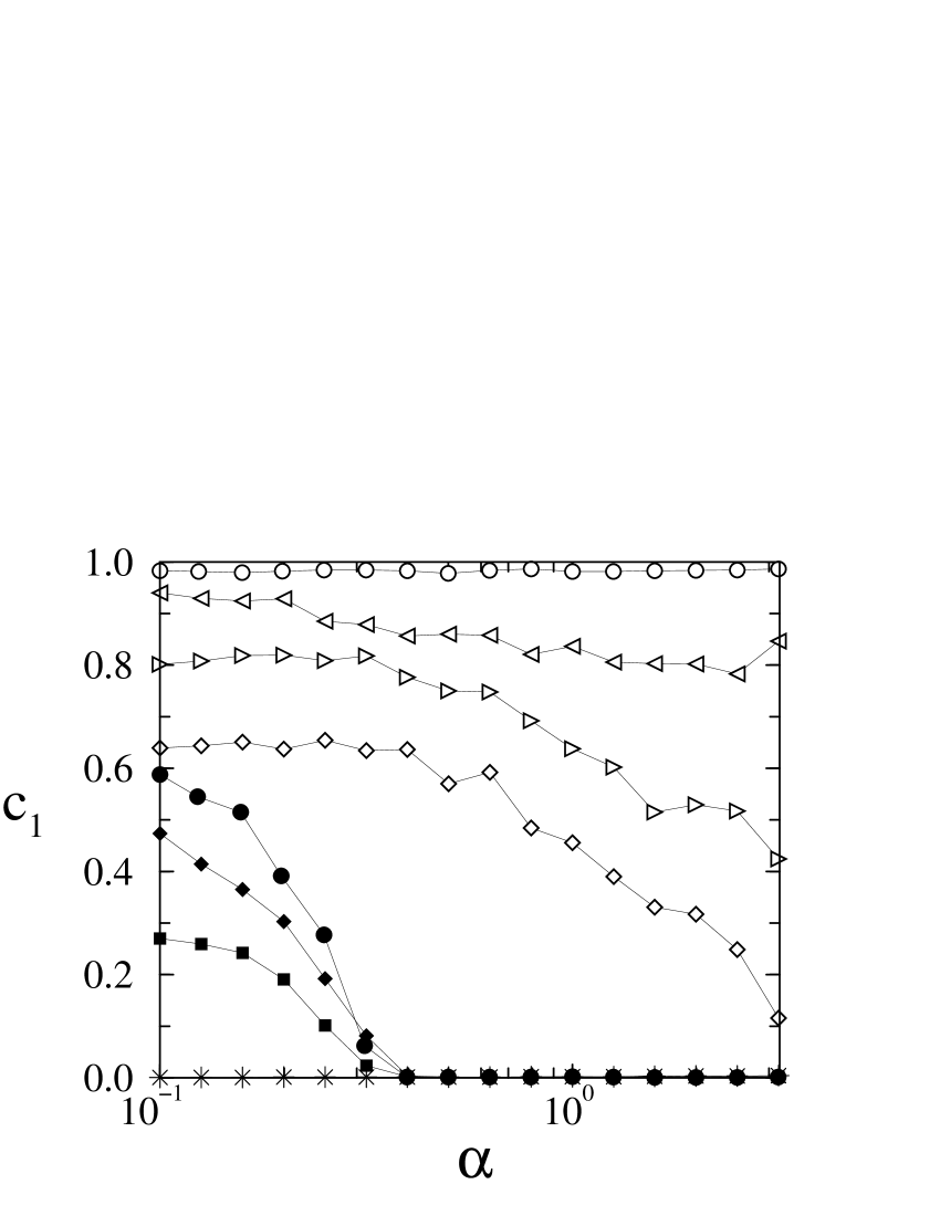
Figure 11: Amplitude of oscillations of the (unconditional) spin-spin correlation function of the on-line game with adaptation allowed only every $M$ time steps. Oscillations are of period $2M$. All data is from simulations, the lines connecting the markers are guides to the eye. Solid symbols: $\rho=1/2$ (squares $M=10P$, diamonds $M=25P$, circles are the data for the batch limit, plotted for comparison, see also Fig. 5). Open symbols: $\rho=0$ (diamonds $M=25P$, right triangles $M=100P$, left triangles $M=1000P$, circles are the data for the batch limit). All simulations are performed at $P=50$ and run for $10^{6}$ on-line steps, averages over $20$ realisations of the disorder are taken disclaimer . Stars are the data for randomized updating ($\rho=0$, $M=10P$, see Fig. 12 for simulation details). No oscillations are found in this case.

Finally we have performed numerical simulations on MGs with asynchronous, random timing of adaptation. Choosing $M\geq{\cal O}(P)$ and allowing all agents independently and randomly with probability $1/M$ to update their strategy preferences at a given on-line step, while still updating their score difference at each step, generates a batch-like model with asynchronous updating. As depicted in Fig. 11 the randomization of the updates removes the oscillations in the spin-spin correlation functions of the batch game. The corresponding volatilities are virtually identical to those of the corresponding on-line games above $\alpha_{c}$, in particular we find $\sigma^{2}=1$ for $\alpha>1$ in the game with random updating and full anti-correlation, see Fig. 12. In the non-ergodic phase the effect of the stochastic updating is a gradual reduction of the volatility.

5 Mixed population of speculators and producers

The theory of section 3 allows one in principle to study the batch MG for an arbitray distribution $P(\rho)$ of correlation parameters. While the previous section dealt only with the case of unimodular distributions, we will now use the above formalism to study a mixed population of ‘speculators’ and ‘producers’ ChalMarsZhan00 . While a speculator is defined as a normal agent (holding two strategies), a producer is an agent with limited choice and has only one single strategy at his or her disposal (or equivalently two identical strategies, corresponding to full correlation, $\rho=1$). A detailed analysis of the statics of games with such mixed populations is contained in ChalMarsZhan00 . In this final section before our conclusions we will complement this work by a study of the dynamics of such models, and will demonstrate that the dynamical theory reproduces the results of the static replica analysis. The interplay of producers and speculators is also discussed in a different context in grandcangf , where so-called grand-canonical MGs are considered; see also MGbook2 for further details.

We will consider an ensemble of $N$ agents, consisting of $(1-x)N$ speculators (with correlation $0\leq\rho<1$ between their strategies) and $xN$ producers, where $0\leq x<1$. This corresponds to a choice

$$P(\rho^{\prime})=(1-x)\delta(\rho^{\prime}-\rho)+x\delta(\rho^{\prime}-1)$$ (47)

in the above generating functional calculation. As before, the parameter $\alpha=P/N$ is defined as the ratio between the number of patterns and the total number of agents. Using Eqs. (25) and (26) we find

$$c = \frac{1-\rho}{1-\overline{\rho}}(1-x)c(\rho)$$ (48)

$$\chi = \frac{1-\rho}{1-\overline{\rho}}(1-x)\chi(\rho),$$ (49)

where $\overline{\rho}=(1-x)\rho+x$. $c$ and $\chi$ are then determined self-consistently using expressions (23) and (24) for $c(\rho)$ and $\chi(\rho)$. We have checked and confirmed these analytical results for $c$ against simulations for some choices of the model parameters, but do not report the numerical data here. After some more algebra we find

$$\chi=\left(\frac{\alpha/(1-x)}{{\rm erf}\left(\lambda/\sqrt{2}\right)}-1\right)^{-1},$$ (50)

where $\lambda$ is fixed as the root of the equation

$$\sqrt{\frac{2}{\pi}}\frac{e^{-\lambda^{2}/2}}{\lambda}+\left(1-\frac{1}{\lambda^{2}}\right){\rm erf}\left(\frac{\lambda}{\sqrt{2}}\right)+\frac{\alpha/(1-x)}{\lambda^{2}}$$ (51)

$$= \frac{1}{(1-\rho)(1-x)}.$$

From this we locate the onset of diverging integrated response as

$$\alpha_{c}=(1-x){\rm erf}\left(\frac{\lambda_{c}}{\sqrt{2}}\right),$$ (52)

where $\lambda_{c}$ solves

$$\sqrt{\frac{2}{\pi}}\frac{e^{-\lambda_{c}^{2}/2}}{\lambda_{c}}+{\rm erf}\left(\frac{\lambda_{c}}{\sqrt{2}}\right)=\frac{1}{(1-\rho)(1-x)}.$$ (53)

Note that $\alpha_{c}/(1-x)$, depends only on the combination $(1-\rho)(1-x)$. The resulting phase diagram is depicted in Fig. 13. The above equations obtained from the generating functional analysis agree with the corresponding results from the replica calculation, as presented in ChalMarsZhan00 .

Finally the generating functional approach allows one to study the influence of decision noise on the phase diagram and behaviour of MGs CoolHeimSher01 . A corresponding calculation for mixed populations of producers and speculators shows that multiplicative noise generally reduces the value of $\alpha_{c}/(1-x)$, i.e. that the range of the ergodic phase is increased when the trading decisions of the producers are made stochastically to a certain degree GallaThesis . This shift of $\alpha_{c}/(1-x)$ becomes more pronounced as the noise level is increased. A similar effect was previously also observed in MGs in which the agents trade on different time scales DeMa03 .

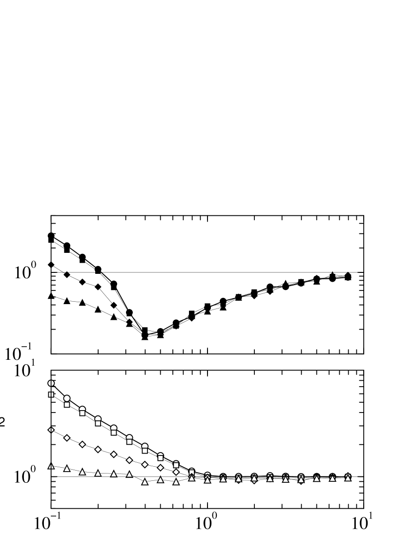
Figure 12: Volatility of the game with randomized, asynchronous strategy updating (allow for strategy switches with probability $1/M$ at each on-line step, independently for different agents). Upper panel: uncorrelated strategies ($\rho=1/2$), lower panel: anti-correlated strategies ($\rho=0$). All data is from simulations at $P=50$, the top most curves (circles) are for $M=1$ (corresponding to the on-line game), squares $M=0.1P$, diamonds $M=P$, triangles $M=10P$. Simulations are started from tabula rasa initial conditions and run for $200M$ on-line steps ($2000M$ steps for $M=0.1P$), all data is averaged over at least $10$ realisations of the disorder. The horizontal lines mark the random trading limit, $\sigma^{2}=1$, in both panels disclaimer2 .

6 Concluding remarks

We have presented an analysis of the dynamics of minority games with diversified strategies. Generating functional techniques can be used to turn the coupled dynamics of $N$ interacting agents with heterogeneous strategy correlations into an effective single-particle problem. The general case of heterogeneous correlation parameters $\rho_{i}$ of the population of agents (drawn from a distribution $P(\rho)$) is reflected in the fact that one finds an ensemble of single agent processes as the final outcome of the theory, as opposed to just one effective single-agent process for the case of uniform correlation parameter ($\rho_{i}=\rho$ for all $i$).

In section 5 of this paper we have used the developed formalism to study mixed populations of ‘speculators’ and ‘producers’. The dynamical approach leads to order parameter equations which are identical to those obtained previously from replica analyses of such models, and accordingly the phase diagrams obtained from the statics and dynamics coincide. In general one finds that adding producers to the MG increases the range of the ergodic phase of the game.

The main focus of our study, however, has been the further analysis of the dynamical effective single-agent problem for the cases of batch and on-line games with unimodal distributions of the strategy correlations, along with numerical simulations and complementing the analysis of the statics of such games previously presented in ChalMarsZhan00 .

We find that the model with uniform, but general correlation parameter $\rho$ exhibits intriguing features, with similarities, as well as crucial differences, compared to the game with uncorrelated strategies ($\rho=1/2$).

The main common features of the games with general correlation parameter are (a) the existence of two distinct phases in both the on-line and batch games for all $0\leq\rho<1$, with an ergodic state for $\alpha>\alpha_{c}(\rho)$, in which no dependence on initial conditions is found, and a non-ergodic phase below $\alpha_{c}(\rho)$, in which the nature of the stationary state depends on the configuration from which the dynamics is started; (b) persistent oscillations are present in the non-ergodic phases of both the batch and the on-line games for all $\rho$. Above $\alpha_{c}(\rho)$, oscillations are absent in on-line games with arbitrary correlation parameter $0\leq\rho<1$, and in batch games as long as $\rho>0$; (c) for $0<\rho<1$ the transition point between the two phases is marked by a minimum of the volatility $\sigma^{2}=\sigma^{2}(\alpha)$ in both the batch and on-line games; (d) we find analytically that the persistent order parameters in the stationary ergodic state and the phase diagram do not depend on the details of the update rules (batch versus on-line learning) and that they agree with those calculated within the replica symmetric approximation; (e) no oscillations are found in simulations of games with random asynchronous updating (for neither uncorrelated nor anti-correlated strategies), while at the same time a reduction of the volatility in the non-ergodic phases of such games is observed.

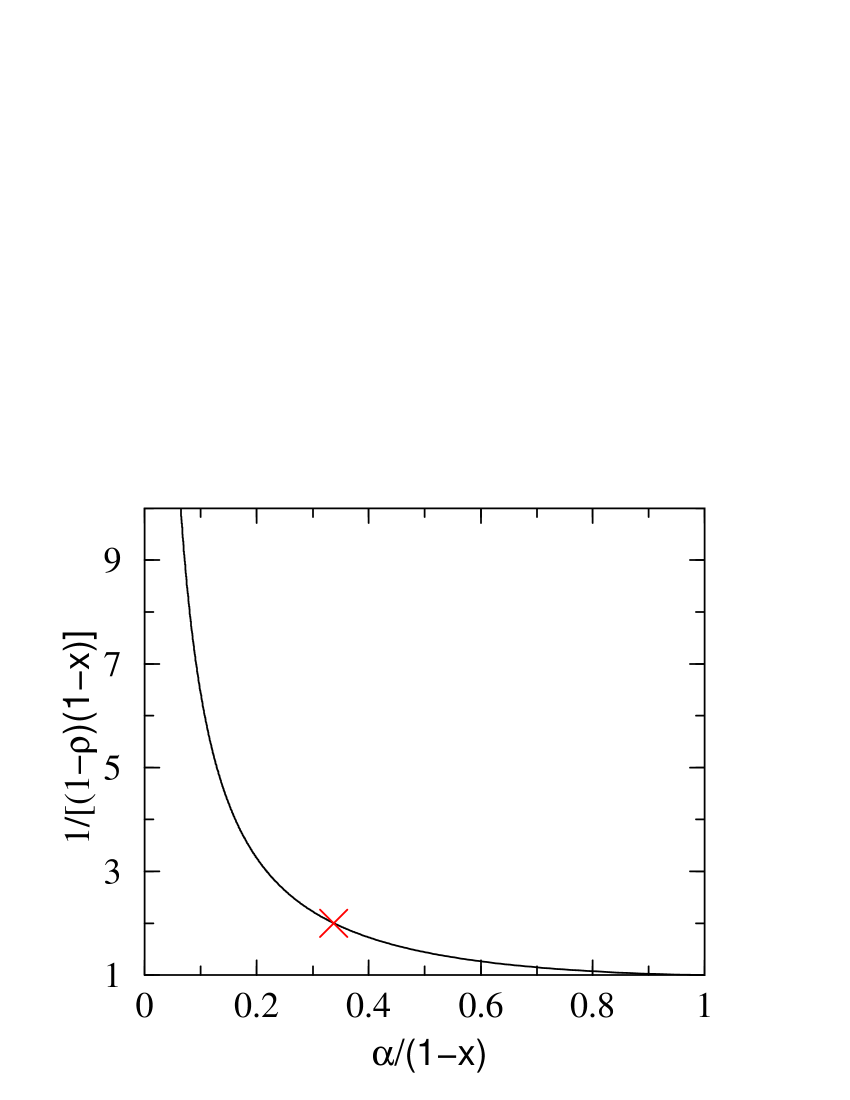
Figure 13: Phase diagram of the batch MG with a mixed population of speculators and producers. The line in the $(\alpha/(1-x),1/[(1-x)(1-\rho)])$-plane is given by (52). The cross marks the location of the phase transition in the standard game $(q=0,\rho=0.5)$.

However, the study of games with differently correlated strategies and different timings of adaptation also reveals some new features and striking differences between on-line and batch games, which up to now have not been discussed systematically in the literature. These new issues may be summarised as follows: (i) the dynamics of the batch game with fully anti-correlated strategies, $\rho=0$, appears different from the batch games with $0<\rho<1$ and from the on-line game with $\rho=0$, as in the batch game at $\rho=0$ oscillations of the form $C(\tau)=(-1)^{\tau}$ are found for all $\alpha$ and not only in the low-$\alpha$ phase; for tabula rasa initial conditions the volatility $\sigma^{2}$ of the batch game is a smooth function of $\alpha$ without any minima or turning points. Nevertheless we find that the game with fully anti-correlated strategies is in a non-ergodic state for $\alpha<\alpha_{c}(\rho=0)=1$ for both batch and on-line learning rules, with the usual dependence of macroscopic order parameters on initial conditions in this regime; (ii) the volatilities in batch and on-line games deviate increasingly from each other as the correlation parameter $\rho$ is lowered; by allowing the agents to update their strategy preferences synchronously only once every $M$ steps it is possible to interpolate smoothly between the on-line and batch limits, $M=1$ and $M\geq{\cal O}(\alpha N)$, respectively; (iii) the available approximations for the volatilities of batch MGs, neglecting the retarded self-interaction of fickle agents, become unreliable in this regime of anti-correlated strategy assigments. Thus, care has to be taken whenever these approximations are applied to other extensions of the conventional batch MG. The corresponding approximations in the on-line case, based on discarding transient contributions to the response and correlation functions, however, appear to be valid above $\alpha_{c}(\rho)$ for all values of $\rho$, even in the case of full anti-correlation.

References

- (1) Challet D and Zhang Y-C 1997 Physica A 246 407
- (2) Challet D, Marsili M and Zhang Y-C 2000 Physica A 276 284
- (3) Challet D, Marsili M and Zecchina R 2000 Phys. Rev. Lett. 84 1824
- (4) Marsili M, Challet D and Zecchina R 2000 Physica A 280 522
- (5) Garrahan J P, Moro E and Sherrington D 2000 Phys. Rev E 62 R9
- (6) Heimel J A F and Coolen A C C 2001 Phys. Rev. E 63 056121
- (7) Marsili M and Challet D 2001 Phys. Rev. E 64 056138
- (8) Savit R, Manuca R and Riolo R 1999 Phys. Rev. Lett. 82 2203
- (9) Cavagna A 1999 Phys. Rev. E 59 R3783
- (10) Coolen A C C 2005 J. Phys. A: Math. Gen. 38 2311
- (11) Heimel J A F, De Martino A 2001 J.Phys. A: Math. Gen. 34 L539
- (12) De Martino A, Giardina I, Mosetti G 2003 J. Phys. A 36 8935
- (13) De Martino A 2003 Eur. Phys. J. B 35 143
- (14) Galla T, Coolen A C C, Sherrington D, J.Phys A: Math. Gen. 36 11159
- (15) Galla T 2005 J. Stat. Mech. P01002
- (16) Coolen A C C, Heimel J A F and Sherrington D 2001 Phys. Rev.E 65 016126
- (17) Coolen A C C 2003 Markov Proc. Rel. Fields 9 177
- (18) Moro E 2004 (to appear in in Advances in Condensed Matter and Statistical Mechanics, ed. E. Korutcheva and R. Cuerno), preprint cond-mat/0402651
- (19) Challet D, Marsili M, Zhang Y-C 2005 Minority Games, Oxford University Press
- (20) Coolen A C C 2005 The Mathematical Theory of Minority Games, Oxford University Press
- (21) Coolen A C C and Heimel J A F 2001 J. Phys. A: Math. Gen. 34 10783
- (22) Sherrington D and Galla T 2003 Physica A 324 25
- (23) Garrahan J P, Moro E, Sherrington D 2001 Quantitative Finance1 246
- (24) Yip K F, Hui P M, Lo T S, Johnson N 2003 Physica A 321 318
- (25) Eissfeller H and Opper M 1992 Phys. Rev. Lett. 68, 2094
- (26) Challet D, Marsili M 1999 Phys. Rev. E 60 R6271
- (27) Coolen A C C 2001, in Handbook of Biological Physics Vol 4 597 , Elsevier Science, eds F Moss and S Gielen, cond-mat/0006011
- (28) Heimel J A F 2001, PhD thesis, King’s College London
- (29) Mosetti G, Challet D, Marsili M, Zhang Y-C 2005 (in preparation)
- (30) Challet D 1999, PhD thesis, University of Fribourg
- (31) Challet D, De Martino A, Marsili M, Perez Castillo I 2004, preprint cond-mat/0407595
- (32) We measure in the stationary state as , where corresponds to effective updates, i.e. on-line steps. While the data for the uncorrelated case () does not seem to exhibit any strong dependence on the sample size , the running time or the details of the numerical procedure of determining in the simulations, we find that the quantitative values of the data for the uncorrelated case () can depend on these parameters. This does not, however, affect the key qualitative observation of an increasing oscillation amplitude as is increased.
- (33) The data for and appears to lie (slightly) below the random trading limit in an interval around . This seems to persist also for larger values of or and/or for longer running times. It is at present unclear whether this constitutes a systematic effect or whether it is an artifact due to limitations in the numerical simulations. Note also that similar observations were made for the on-line case with real market histories ( and ) ChalletThesis .
- (34) Galla T 2004, D.Phil. thesis, University of Oxford