Structural Disorder Induced Polaron Formation and Magnetic Scattering in the Disordered Holstein-Double Exchange Model

Abstract

In this paper we present results on the disordered Holstein-Double Exchange model, explicitly in three dimension and ‘metallic’ densities, obtained by using a recently developed Monte Carlo approach. Following up on our earlier paper, cond-mat 0406085, here we provide a detailed microscopic picture of the thermally driven metal-insulator transition (MIT) that arises close to the ferromagnet to paramagnet transition in this problem. This paper is focused mainly on the ‘diagnostics’, clarifying the origin of the effective disorder that drives the MIT in this system. To that effect, we provide results on the thermal evolution of the distributions of (i) lattice distortions, (ii) the net ‘structural disorder’ and (iii) the ‘hopping disorder’ arising from spin randomness feeding back through the Hunds coupling. We suggest a phenomenology for the thermally driven MIT, viewing it as an ‘Anderson-Holstein’ transition.

1 Introduction

The Holstein-Double Exchange (H-DE) model has been the focus of recent attention because it can help clarify the combined effect of strong electron-phonon (EP) interaction and strong electron-spin coupling that operates in the manganites, La_1-xCa_xMnO₃, say [1]. The detailed microscopic model for manganites is rather complicated. Let us start by describing this model, and argue how successive reduction to the disordered H-DE model retains some of the essential physics.

The comprehensive tight binding model for perovskite manganites, neglecting oxygen orbitals, etc, is

$$H = \sum_{\langle ij\rangle\sigma}^{\alpha\beta}t_{ij}^{\alpha\beta}c^{\dagger}_{i\alpha\sigma}c^{~{}}_{j\beta\sigma}+\sum_{i}\epsilon_{i}n_{i}-J_{H}\sum_{i}{\bf S}_{i}{\bf.}{\hat{\bf\sigma}_{i}}$$ (2)

$$-\lambda\sum_{i}{\bf Q}_{i}{\bf.}{\hat{\bf\tau}_{i}}+H_{\mathrm{stiff}}+H_{\mathrm{ph-dyn}}+H_{\mathrm{Hubb}}$$

The $t_{ij}^{\alpha\beta}$ are hopping between doubly degenerate Mn $e_{g}$ levels at neighbouring sites, $\epsilon_{i}$ refers to weak substitutional disorder, and $J_{H}$ is the strong Hunds coupling between the $e_{g}$ electrons and the $S=3/2$ ‘core spin’ ($t_{2g}$ electrons). The ‘orbital moment’, ${\bf\tau}_{i}$, of the $e_{g}$ electrons is Jahn-Teller coupled to the octahedral distortion parameter ${\bf Q}_{i}$, through the EP coupling $\lambda$. $H_{\mathrm{stiff}}$ is the stiffness of the lattice. In its simplest form it is $\sim(K/2)\sum_{i}Q_{i}^{2}$, but in reality is of ‘cooperative’ character, i.e, involves phonon degrees of freedom in more than one octahedra. The phonons are quantum variables, with intrinsic dynamics arising from $H_{\mathrm{ph-dyn}}\sim P^{2}/(2M_{Q})$, where $P$ is the momentum and $M_{Q}$ the mass of the relevant oscillator. Finally, the $x=0$ state in the manganites is a Mott insulator, arising (partly) from large on site ‘inter-orbital’ Hubbard repulsion, $H_{\mathrm{Hubb}}\sim U^{\prime}\sum_{i,\alpha\neq\beta}n_{i\alpha}n_{i\beta}$.

The electron-phonon, electron-spin and Hubbard interactions are all large $\gg t$, where $t$ is the typical hopping scale in the problem, and therefore beyond the range of perturbation theory. The detailed model, unfortunately, is far too complex for the present methods of many body theory, if it were to be handled in a realistic three dimensional situation. However, it is possible to simplify the model somewhat, recognising that (i) at large doping of the Mott insulator, e.g, $x\sim 0.3-0.4$, the Hubbard interaction probably does not have a qualitative effect, (ii) the phonons are in the adiabatic regime, with typical frequency $\omega_{\mathrm{ph}}\ll t$ and, as a first approximation, we can explore the adiabatic limit $\omega_{\mathrm{ph}}=0$, and (iii) the $S=3/2$ may be approximated as a ‘classical’ spin.

This still leaves us with the problem of (disordered) electrons strongly coupled to (classical) phonon and spin degrees of freedom. The qualitative effects in such a system include (i) magnetic order, typically ferromagnetism, arising from Hunds coupling and electron delocalisation, (ii) the possibility of polaron formation if the EP coupling is sufficiently large compared to the kinetic scale, and (iii) the phase competetion between different kinds of long range order. These complexities, observed experimentally in the manganites, can be recovered already at the level of the Jahn-Teller-Double Exchange (JT-DE) model, neglecting $H_{\mathrm{ph-dyn}}$ and $H_{\mathrm{Hubb}}$.

The JT-DE model was explored by Millis et al., [2] within dynamical mean field theory (DMFT), and later by Dagotto and coworkers [3] using real space Monte Carlo (MC) tecniques. The DMFT study could demonstrate a thermally driven metal-insulator transition (MIT), as observed in La_0.7Ca_0.3MnO₃, although only at $x=0.5$. The MC studies, on the other hand, have gone a long way in clarifying the various phases in the JT-DE model, but the severe finite size handicap has prevented estimate of transport properties.

If we tentatively accept that the essential physics in the manganites arises from the general interplay of EP coupling and double exchange, then the JT-DE model can be further reduced to a one band version: the Holstein-Double Exchange model, defined further on. Indeed, it was studied early on [4], simultaneously with the JT-DE work of Millis et al., within a mean field approximation, to clarify the effect of EP coupling on the ferromagnetic $T_{\mathrm{c}}$. That work did not address transport properties. More recently the H-DE model has been studied via many body CPA approximations [5] and through direct Monte Carlo simulation [6]. The MC study does find a thermally driven MIT but only at low carrier density. In addition, all these studies neglect the effect of quenched disorder which should have a dramatic impact [7] in a system with strong EP coupling.

The effect of disorder in ‘manganite models’ have in fact been discussed [8, 9], but the focus has been on its impact on phase competetion and bicriticality. Disorder can lead to nanoscale cluster coexistence near a first order phase boundary [10] and much of the disorder related theory has concentrated on modelling this phenomena. While this is a vital issue, there is a completely independent effect of disorder that shows up in systems with strong EP coupling. Disorder can induce polaron formation, even below the polaronic threshold for ‘clean’ systems, and drastically modify the residual resistivity, the optical spectral weight, and in fact the entire transport response. Manganite data testifying to these effects abound in the literature, but there has been no theoretical effort to understand these phenomena.

2 Experiments in the Manganites

In the manganites, A_xA’_1-xMnO₃ say, the physics is controlled by varying $x$, or the mean A-A’ site cation radius $r_{A}$, or the cation disorder $\sigma_{A}$, arising from size mismatch. Since the parameters $r_{A}$ and $\sigma_{A}$ themselves depend on $x$, it is best to focus on data at a fixed doping level. In this spirit, experimenters have used chemical variation at fixed $x$, varying both $r_{A}$ (which controls the electronic bandwidth) and $\sigma_{A}$ [11, 12]. Pressure experiments, on the other hand involve variations in the bandwidth, keeping the disorder constant [13, 14]. Finally, the effect of disorder has been explored, keeping $x$ and $r_{A}$ fixed, varying only $\sigma_{A}$ [15, 16].

The main conclusion of these studies is that (i) large $r_{A}$ systems, La_1-xSr_xMnO₃, are ‘canonical DE magnets’, with a saturated ferromagnetic ground state, ‘metallic’ resistivity at all temperature, and modest magnetoresistance (MR) near $T_{\mathrm{c}}$, (ii) reducing $r_{A}$, as in La_1-xCa_xMnO₃, maintains a saturated ferromagnetic ground state, but there is a thermally driven MIT near $T_{\mathrm{c}}$, with associated colossal magnetoresistance, and a pseudogap in density of states (DOS), (iii) further reduction in $r_{A}$ as in La_1-x-yPr_yCa_xMnO₃, leads to a non saturated ferromagnetic ground state, mixed phase tendency, nanoscale clusters (depending on disorder), a field driven insulator-metal transition at zero temperature, and large MR over a wide temperature range. All these occur with only a few percent change in $r_{A}$.

These data define the problem for a ‘global’ description of the effects seen in the manganites. With small variation in electronic bandwidth (or inversely the EP coupling), $\sim 10\%$, a theory should be able to reproduce the suppression in $T_{\mathrm{c}}$, the dramatic changes in transport character, reduction of low frequency optical spectral weight, sharply enhanced residual resistivity, and emergence of a pseudogap features in the DOS. Simultaneously it should reproduce similar effects if the quenched disorder were increased, remaining at fixed EP coupling and bandwidth.

In our earlier paper [17] we had solved the disordered Holstein-Double Exchange ($d$-H-DE) model and qualitatively reproduced all the trends above (except magnetic phase competetion, which requires additional antiferromagnetic coupling). In this paper we focus on a generic point in parameter space, where there is a thermally driven MIT, and try to provide a detailed microscopic picture for the transition.

3 Model and Method

The $d$-H-DE model, with classical spins and phonons, is defined by:

$$H = -t\sum_{\langle ij\rangle\sigma}c^{\dagger}_{i\sigma}c^{~{}}_{j\sigma}+\sum_{i}(\epsilon_{i}-\mu)n_{i}-J_{H}\sum_{i}{\bf S}_{i}.{\sigma}_{i}$$ (4)

$$~{}~{}~{}~{}~{}~{}~{}~{}~{}-\lambda\sum_{i}n_{i}x_{i}+{K\over 2}\sum_{i}x_{i}^{2}$$

Here the $t$ are nearest neighbour hopping on a simple cubic lattice, $\epsilon_{i}$ is the quenched binary disorder, with value $\pm\Delta$, and $J_{H}$ is the Hunds coupling. $\lambda$ is the EP interaction, coupling electron density to the local distortion $x_{i}$, and $K$ is the stiffness of the lattice. The basic parameters in the problem are $\Delta/t$, $\lambda/t$, electron density $n$, and temperature $T$. We work in the limit $J_{H}/t\rightarrow\infty$. We also set $K=1$, and measure energy, frequency, $T$, etc, in units of $t$.

For $J_{H}/t\rightarrow\infty$, the Hunds coupling acts as a constraint, orienting the electron spin at a site parallel to the core spin (and projecting out the anti-parallel component) leading to the following spinless fermion model:

$$H \equiv -\sum_{\langle ij\rangle}(t_{ij}\gamma^{\dagger}_{i}\gamma_{j}~{}+~{}h.c~{})+\sum_{i}\xi_{i}n_{i}+{K\over 2}\sum_{i}x_{i}^{2}$$ (5)

$$t_{ij} = ~{}~{}t(\cos{\theta_{i}\over 2}\cos{\theta_{j}\over 2}+i~{}\sin{\theta_{i}\over 2}\sin{\theta_{j}\over 2}e^{i(\phi_{i}-\phi_{j})})$$ (6)

(7)

$$\xi_{i} = \epsilon_{i}-\mu-\lambda x_{i}$$ (8)

The $\gamma,\gamma^{\dagger}$ are spinless fermion operators, corresponding to the ‘parallel’ spin projection of the original electrons. $\xi_{i}$ is the net ‘potential’ seen by the electrons, while the hopping ‘disorder’ is controlled by $\theta_{i}$ and $\phi_{i}$, the polar and azimuthal angles, respectively, of ${\bf S}_{i}$.

The problem involves strong coupling and disorder, and needs to handle thermal fluctuations. We use a recently developed Monte Carlo technique [18] based on a “travelling cluster approximation” (TCA) to anneal the classical variables. This allows us to use system sizes $N\sim 10^{3}$ and address the MIT in the model.

After equilibriating the phonon and spin degrees of freedom for a specified set of parameters, disorder realisation, and $T$, we compute the following: (i) transport properties, adapting a scheme [19] which now uses electronic eigenfunctions in the annealed background, and Fermi factors, for $T\neq 0$, (ii) DOS, (iii) the thermally averaged lattice distortion, as well as (iv) the distribution of net ‘structural disorder’ and hopping disorder, and (v) spatially resolved information on density distribution, $n_{\bf r}$, and the magnetic correlation, $f_{mag}({\bf r})=\sum_{{\bf r}^{\prime}}\langle{\bf S}_{\bf r}.{\bf S}_{{\bf r}^{\prime}}\rangle$, where ${\bf r}$, ${\bf r}^{\prime}$ are nearest neighbours.

4 Results

In our earlier, main paper [17], we have provided the $n-T$ phase diagram in the clean limit for various $\lambda$, while the transport, spectral and optical properties were shown for $n=0.3$ varying the EP coupling and disorder. We demonstrated a thermally driven MIT over a wide parameter regime in $\lambda-\Delta$ but did not have room to provide a detailed microscopic picture of the ‘thermal disorder’ that drives the MIT. This paper focuses on a single, generic, point in parameter space $n=0.3$, $\lambda=2.0$, $\Delta=0.6$ and tracks the $T$ dependence of the distribution of effective disorder as well as the spatially inhomogeneous underlying state.

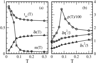
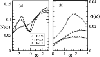
Figure 1: Panel $(a).$ shows the variation in the magnetisation, $m(T)$, the mean magnitude of the hopping amplitude, $t_{av}(T)$, and the r.m.s fluctuation in the hopping, $\delta t(T)$. Panel $(b).$ shows the scaled resistivity, $\rho(T)$, the scaled variance of the lattice distortion, $\delta x^{2}$, and the variance of the effective disorder $\delta\eta^{2}$.

Figure 2: (a) The low energy density of states, and (a)  the low frequency optical conductivity, with varying temperature.

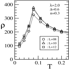
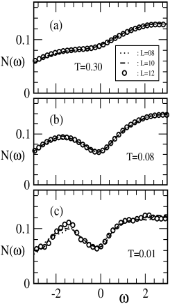
Figure 3: The temperature dependence of the ‘d.c’ resistivity at three system sizes, $L=8,~{}10,~{}12$, with $N=L^{3}$.

Figure 4: Size dependence in the low frequency density of states, showing the stability of the pseudogap feature. System sizes, $N=L^{3}$ with $L=8,~{}10,~{}12$, as in Fig.3.

If the thermally driven MIT in the manganites is a “localisation transition”, rather than simple “band splitting”, a real space understanding of the phenomena should be of crucial importance.

Figure 1(b) shows the resistivity at our chosen parameter point. Figure 1(a) shows the variation in magnetisation, $m(T)$, the spin disorder induced suppression of the average, $t_{av}=\langle|t_{ij}|\rangle$, and the r.m.s fluctuation $\delta t(T)$ in the hopping distribution.

The evolution of the mean square lattice distortion, as well as the effective structural disorder arising from $\epsilon_{i}-\lambda x_{i}$ are shown in panel (b). The full distribution of these disorder is shown in Fig. 5. The kink like feature in $\rho(T)$ is a consequence of a discrete set of points sampled in $T$. Denser sampling reveals a more continuous change in character.

Apart from the MIT, whose detailed description is our primary focus in this paper, Fig. 2(a) shows the thermal evolution of the low energy DOS, while Fig. 2(b) shows the low frequency optical conductivity. The two features to note are (i) the non monotonic $T$ dependence of the low energy DOS (the ‘dip’ deepens initially with increasing $T$ and then fills up) and (ii) the strongly non Drude nature of the optical response even at $T=0$. The resistivity and DOS had been shown in our earlier paper [17]. In what follows we want to focus on the (annealed) disorder that is responsible for these physical effects. The finite size effects in this problem are rather weak, as borne out by the size dependence of the resistivity in Fig. 3, and the density of states, Fig. 4.

Effects for $T\rightarrow 0$: Figure 1(b) shows that there are lattice distortions of fairly large magnitude even at $T=0$, in the fully polarised ferromagnetic state. An understanding of this can be obtained by studying the disordered spinless Holstein model [20] where we observe that close to a (collective) polaronic instability, even weak disorder can induce large lattice distortions and localise a fraction of charge carriers. This phase differs from a polaronic insulator in that there are still extended states that survive close to the Fermi level. The DOS shows signature of this partial polaronic trapping (i.e a pseudogap), and the optical response has the non Drude character typical of electrons in a strongly disordered background.

Figure 5 shows the actual distributions, of lattice distortions, $x_{i}$, the net potential $\eta_{i}=\epsilon_{i}-\lambda x_{i}$, and the magnitude of hopping, $|t_{ij}|$. The quenched disorder is binary with value $\pm 0.6$. Starting with panel (c), the hopping distribution $P(|t|)$ tends to a $\delta$ function as $T\rightarrow 0$ since all spins are aligned. In this regime the physics is controlled purely by the effective structural disorder. The $P(x)$ distribution is bimodal, with significant weight near $x\sim\lambda/K=2$, which would arise for strongly localised particles. There is also a peak related to the original clean Fermi liquid, surviving near the origin.

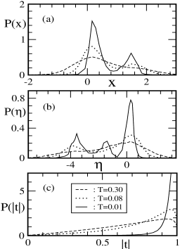
Figure 5: Panel (a): $P(x)$ the distribution of lattice distortions, averaged thermally and over the system, (a) the distribution of the effective potential, $\eta_{i}=\epsilon_{i}-\lambda x_{i}$, seen by the electrons, and (c) the distribution in the magnitude of the hopping, essentially the nearest neighbour correlation $\sqrt{1+{\bf S}_{i}.{\bf S}_{j}}$.

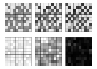
Figure 6: The view on the top surface of a $10^{3}$ system. The row above shows the thermally averaged density profile, $n_{\bf r}$, at $T=0.01,0.08,0.30$ (right to left). The row below shows the nearest neighbour averaged magnetic correlation: $f_{mag}({\bf r})=\sum_{{\bf r}^{\prime}}\langle{\bf S}_{\bf r}.{\bf S}_{{\bf r}^{\prime}}\rangle$, for the same sequence of temperatures.

We can crudely estimate the number of strongly localised carriers in terms of $\int_{x_{\mathrm{min}}}^{\infty}dxP(x)$ where $x_{\mathrm{min}}=1.2$ is the (approximate) upper limit of distribution at weak disorder, $\Delta=0.2$, Fig. 7. This area is roughly $0.2-0.25$ at $\Delta=0.6$. Since the electron density itself is $n=0.3$ this suggests that a large fraction of carriers have collapsed into “polaronic” states. The density profile at $T=0.01$, Fig. 6, top right, confirms this picture. That not all particles are localised is borne out by the residual resistivity, $\rho(0)$. We have checked that large $L$ extrapolation of our results (verified using $N=6^{3}-12^{3}$) still leads to finite $\rho(0)$.

The $P(\eta)$ distribution, at $T=0$, is more complex than $P(x)$, and is more relevant for understanding the ‘landscape’ in which the electrons move. As a starting point we can imagine three kinds of sites: (i) sites with $\epsilon_{i}=\pm\Delta$, with weak distortions and no ‘overdensity’, these sites would be continuation of the clean Fermi liquid, call them $\eta_{FL}$, (ii) sites with $\epsilon_{i}=-\Delta$ and some large distortion (call these $\eta^{-}$) and (iii) sites with $\epsilon_{i}=+\Delta$ and moderately large distortions ($\eta^{+}$).

The $x_{i}$ for a ‘site localised’ electron is $\sim\lambda/K=2$, so the $\eta^{-}$ sites would have magnitude $\approx-\Delta-\lambda^{2}/K=-4.6$. In fact the ‘polarons’ are not quite site localised, so $\eta^{-}$ would be somewhat less: consistent with the left peak in Fig. 5(b). As for the $+\Delta$ sites, these could have been avoided by the trapped particles if the carrier density was low. However at $n=0.3$, some $+\Delta$ sites also have distortions and an associated overdensity, $\delta n_{\bf r}$, but the magnitude is smaller than that for $-\Delta$ sites.

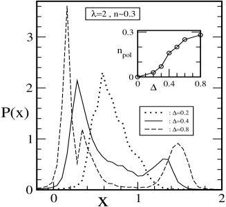
Figure 7: The distribution $P(x,\Delta)$ at $T=0.01$ showing the evolution of the polaronic peak with increasing disorder. Inset: variation in the density of localised carriers, $n_{pol}$, with increasing disorder, staying at $\lambda=2.0$ and fixed electron density, $n=0.3$ We have used $n_{pol}(\Delta)=\int_{x_{\mathrm{min}}}^{\infty}dxP(x,\Delta)$ with $x_{\mathrm{min}}=1.2$.

This happens because locating the localised particles always on $-\Delta$ sites would sometimes require occupancy of adjacent sites. That would inhibit the (virtual) polaron hopping process, and lose kinetic energy. The compromise is to lose some ‘potential energy’ and put carriers on non adjacent sites which may have unfavourable $\epsilon_{i}$. This is the origin of the visible ‘checkerboard’ pattern in Fig. 6, where particles generally prefer to remain on the diagonal with respect to each other. At stronger disorder, pinning would dominate over kinetic energy considerations, and $+\Delta$ sites would be depopulated.

The $P(\eta)$ distribution is of course not $\delta$ functions at $\eta^{\pm}$ or $\eta_{FL}$ and only has a broad three peak character.

Based on the data discussed here, as well as the overall properties presented earlier [17, 20] we suggest the following phenomenology for the $T=0$, spin polarised case: (a) The weak binary disorder tends to create a landscape where electronic eigenfunctions, and the resulting density, $n_{\bf r}$, are weakly inhomogeneous. The strong EP coupling amplifies this inhomogeneity, by generating lattice distortions, leading to a state with a fraction of electronic states strongly localised. Figure 7 shows $P(x)$ for several $\Delta$ at $T=0.01$, and also the inferred density of polaronic states $n_{pol}$ at $n=0.3$. (a) Polaron formation transfers weight in $N(\omega)$ from around $\epsilon_{F}$ to lower energies, creating a pseudogap, and reduces the kinetic energy (or effective carrier count), as visible in the low frequency optical spectral weight [17] $n_{\mathrm{eff}}({\bar{\omega}},T)=\int_{0}^{\bar{\omega}}\sigma(\omega,T)d\omega$, by a factor of 10 (at ${\bar{\omega}}=1$) with respect to the $\Delta=0$ probem. (c) There are, however, delocalised but strongly scattered states which still survive (at moderate $\Delta$): these give rise to finite conductivity at $T=0$, and a ‘metallic’ albeit non Drude response in $\sigma(\omega)$. $(d)$ In between the strongly localised ‘polaronic’ states, and the delocalised states near the Fermi level, there are possible ‘Anderson localised’ states as well, by which we mean states with large localisation length, $\xi_{loc}$. For ‘polaronic’ states $\xi_{loc}\sim 1$.

A quantitative analysis in terms of these three kinds of states is possible, by examining the electronic eigenfunctions (or inverse participation ratio) in the annealed background. We leave such discussion for the future.

Effects at finite temperature: We have tried to argue how the interplay of disorder and EP coupling leads to a strongly inhomogeneous state at $T=0$. For ease of argument let us call this a ‘two fluid’ scenario, involving strongly localised states below the Fermi level, and strongly scattered extended states near $\epsilon_{F}$. How does this picture evolve at finite $T$, when the magnetic degrees of freedom also come into play?

The resistivity itself increases quickly with increasing temperature, Fig. 1(b), unlike what is observed in the non magnetic case [20] where the spin disorder does not feed back. We argue that the localised states are now subject to additional ‘hopping disorder’, as evident in Fig. 1(a) and Fig. 5(c), and remain ineffective in the conduction process. In fact, they are localised marginally more due to the additional randomness as the trend in the DOS reveals.

The extended states, which were earlier scattered by the potential fluctuations, $\eta_{i}$, are now also scattered by the bond disorder in $t_{ij}$ and experience reduced mobility. This situation is similar to the previously studied interplay of structural disorder and paramagnetic scattering in the double exchange model [19, 21], where it was found that turning on spin disorder indeed increases the resistivity of the structurally disordered system. That problem, however, dealt with ‘quenched’ structural and magnetic disorder, while both of these are annealed variables in the present problem. Furthermore, as the magnetic disorder increases some of extended states (or, more accurately, the fraction of extended states in a typical equilibrium configuration) reduces. Depending on $\lambda$ and $\Delta$, with increasing $T$ the combined disorder in $t_{ij}$ and $\epsilon_{i}-\lambda x_{i}$ (see eq.(3)) can drive the ‘mobility edge’, $\mu_{\mathrm{c}}(T)$, above the Fermi level. This indeed happens at the parameter point that we considered in this paper, while the full range of possibilities, including a simple ‘metal to metal’ crossover, is detailed in the previous paper [17].

The high temperature ‘insulating’ phase that shows up for $T>T_{MIT}\sim T_{\mathrm{c}}$ is different from a standard ‘Anderson insulator’ for two reasons: (i) the localisation arises from a complex annealed disorder background, and not from an uncorrelated disorder distribution, hence the pseudogap features, and (ii) since the thermal increase in disorder is itself driven by $T$, the mobility gap $\mu_{\mathrm{c}}(T)-\epsilon_{F}$ is always comparable to $T$, so there is no simple activated behaviour in the high temperature resistivity. This is roughly consistent with what is observed in La_0.7Ca_0.3MnO₃, while the MIT is much stronger, and the insulating phase more resistive, in the PrCa systems.

5 Discussion

We have focused till now on our own results on the MIT obtained in the adiabatic $d$-H-DE model. It may be useful to place these results in relation to previous work exploring ‘bicriticality’ in manganite models, and also comment on cooperative lattice effects and quantum fluctuations in spins and phonons.

(i) The connection with bicriticality: The issue of phase competetion, the existence of first order phase boundaries, and the effect of disorder in such a regime has been explored in simple models [8, 9]. The issue was brought to focus by the early work of Dagotto and coworkers [8], who suggested that the presence of disorder near a first order phase boundary between a ferromagnetic metal (FM) and an antiferromagnetic (possibly charge ordered) insulator (AFI) could lead to a pattern of coexisting FM and AFI clusters and percolative transport. The detailed transport properties in such a system, probed within a microscopic theory, were clarified by us [22]. More recently a model involving Double Exchange, Holstein EP coupling, and disorder, has been studied in a two dimensional system, at half-filling, and discovered the “metallisation” of an intermediate coupling charge ordered (CO) phase by weak disorder. Our own results, far from a CO state, suggest how a metal close to a polaronic instability is affected by the presence of weak disorder.

Weak disorder has contrasting roles in these different situations. (a) For a generic first order transition, between a FM and an AFI, say [8, 22] disorder acts to convert “macroscopic” phase separation to meso/nanoscale phase coexistence depending on the strength of the random potential. This harks back to the classic Imry-Ma scenario [23] and a fascinating variety of percolative effects can arise. The key physical effect here is disorder induced cluster formation near a first order transition and does not involve phonons in any essential way. In fact if phonons were to be included there are additional effects of disorder (beyond Imry-Ma) which need to be considered. The second case [9], (a) involves the effect observed in the $n=0.5$ CO system. Here disorder generates a pinning potential, which acts as a random field, and destroys the positional correlations of the CO state. Since the intermediate coupling CO state depends on the periodicity of the CO to generate insulating behaviour, destruction of CO promotes metallisation [9, 24], which we have observed in our 3d study [20] as well. This is disorder induced metallisation of an intermediate coupling CO state. If the EP coupling were large then disorder could still destroy the CO phase but the charge ordered insulator would be converted to a charge disordered polaronic insulator. Our situation, (c) corresponds to a clean metal close to a polaronic instability being converted to a highly resistive state by the effect of disorder. Here disorder induces a polaronic instability. It should be clear that the physical effect in (a) have no essential relation to those in (a) and (c). While it is true that both (a) and (c) arise in the same model, they occur on quite distinct reference states, and the key weak disorder effects are physically very different, despite belonging to the same ‘global’ $\lambda-\Delta-n-T$ phase diagram.

(ii) Order of the MIT: we think the ‘second order’ character of our MIT is due to the effect of noncooperative phonons. If the lattice degrees of freedom were directly coupled, as in the real material, then distortions at one site can have a cascading effect on the other sites, generating an abrupt transition, as indeed observed in one MC study [6].

(iii) Quantum fluctuations in spins and phonons: Our $T=0$ state has no quantum fluctuations (in spins or phonons). While the quantum character of phonons affects the low $T$ resistivity in clean metals, for the disordered strong coupling systems that we consider (with large lattice distortions at $T=0$) quantum fluctuations may not have a qualitative effect. It should be possible to make a perturbative estimate of the effects at small phonon frequency $(\omega_{\mathrm{ph}}/t\ll 1)$, we have not done that yet. Similarly, the system is a fully polarised magnet at $T=0$. Since the effective couplings in the problem are ferromagnetic we do not anticipate a significant renormalisation in magnetic properties due to quantum spin fluctuations. Finally, by the time $T\sim T_{\mathrm{c}}$, where the MIT occurs, the thermal fluctuations in spins and phonons are far more important than quantum effects.

6 Conclusion

The role of disorder is crucial in the manganites, quite independent of its effect at magnetic bicriticality. This is due to the inherently strong EP coupling in the manganites, which places them close to a polaronic instability. Disorder can partially trigger such an instability. The interplay of disorder and EP coupling controls the resistivity and the ferromagnetic $T_{\mathrm{c}}$. Even at fixed density and $r_{A}$ (or $\lambda$) just increasing disorder can completely change the transport response.

While the present investigation has focused only on the thermally driven metal-insulator transition, the combined effect of electron-phonon coupling, disorder, and an antiferromagnetic coupling (to compete with double exchange) can generate responses that interpolate between the ‘canonical DE magnets’, La_1-xSr_xMnO₃, to thermally driven transitions, La_1-xCa_xMnO₃, all the way to bicriticality and possible nanoscale coexistence, as in La_1-x-yPr_yCa_xMnO₃. A systematic use of our method should clarify the origin, and provide a detailed microscopic description, of the wide variety of transport regimes observed in the manganites.

We acknowledge use of the Beowulf cluster at HRI.

References

- [1] See, e.g, Colossal Magnetoresistive Oxides, edited by Y. Tokura, Gordon and Breach, Amsterdam (2000).
- [2] A. J. Millis, B. I. Shraiman, and R. Mueller, Phys. Rev. Lett. 77 (1996) 175.
- [3] S. Yunoki, A. Moreo, and E. Dagotto, Phys. Rev. Lett. 81 (1998) 5612.
- [4] H. Roder, Jun Zang, and A. R. Bishop, Phys. Rev. Lett. 76 (1996) 1356.
- [5] A. C. M. Green, Phys. Rev. B 63 (2001) 205110.
- [6] J. A. Verges, V. Martin-Mayor, and L. Brey, Phys. Rev. Lett. 88 (2002) 136401.
- [7] D. Emin and M. N. Bussac, Phys. Rev. B 49 (1994) 14290.
- [8] A. Moreo, M. Mayr, A. Feiguin, S. Yunoki, and E. Dagotto, Phys. Rev. Lett. 84 (2000) 5568.
- [9] Y. Motome, N. Furukawa, and N. Nagaosa, Phys. Rev. Lett. 91 (2003) 167204.
- [10] M. Uehara, S. Mori, C. H. Chen and S. -W. Cheong, Nature, 399 (1999) 560, M. Fath, S. Freisem, A. A. Menovsky, Y. Tomioka, J. Aarts and J. A. Mydosh, Science, 285 (1999) 1540.
- [11] E. Saitoh, Y. Okimoto, Y. Tomioka, T. Katsufuji, and Y. Tokura, Phys Rev. B 60 (1999) 10362.
- [12] D. Akahoshi, M. Uchida, Y. Tomioka, T. Arima, Y. Matsui, and Y. Tokura, Phys. Rev. Lett. 90 (2003) 177203.
- [13] H. Y. Hwang, T. T. M. Palstra, S- W. Cheong, and B. Batlogg, Phys. Rev. B 52 (1995) 15046.
- [14] P. Postorino, A. Congeduti, P. Dore, A. Sacchetti, F. Gorelli, L. Ulivi, A. Kumar, and D. D. Sarma, Phys. Rev. Lett. 91 (2003) 175501.
- [15] L. M. Rodriguez-Martinez and J. P. Attfield, Phys. Rev. B 54 (1996) 15622, Phys. Rev. B 58 (1998) 2426.
- [16] A. Maignan, C. Martin, G. Van Tendeloo, M. Hervieu and B. Raveau, Phys. Rev. B 60 (1999) 15214.
- [17] S. Kumar and P. Majumdar, cond-mat 0406085.
- [18] S. Kumar and P. Majumdar, cond-mat 0406082.
- [19] S. Kumar and P. Majumdar, Europhys. Lett. 65 (2004) 75.
- [20] S. Kumar and P. Majumdar, cond-mat 0406084.
- [21] Q. Li, Jun Zang, A. R. Bishop, and C. M. Soukoulis, Phys. Rev. B 56 (1997) 4541.
- [22] S. Kumar and P. Majumdar, Phys. Rev. Lett. 92, (2004) 126602.
- [23] Y. Imry and S.-k. Ma, Phys. Rev. Lett. 35 (1975) 1399.
- [24] C. Sen, G. Alvarez, and E. Dagotto, Phys. Rev. B 70 (2004) 064428.