Singlet-triplet splitting, correlation and entanglement of two electrons in quantum dot molecules

Abstract

Starting with an accurate pseudopotential description of the single-particle states, and following by configuration-interaction treatment of correlated electrons in vertically coupled, self-assembled InAs/GaAs quantum dot-molecules, we show how simpler, popularly-practiced approximations, depict the basic physical characteristics including the singlet-triplet splitting, degree of entanglement (DOE) and correlation. The mean-field-like single-configuration approaches such as Hartree-Fock and local spin density, lacking correlation, incorrectly identify the ground state symmetry and give inaccurate values for the singlet-triplet splitting and the DOE. The Hubbard model gives qualitatively correct results for the ground state symmetry and singlet-triplet splitting, but produces significant errors in the DOE because it ignores the fact that the strain is asymmetric even if the dots within a molecule are identical. Finally, the Heisenberg model gives qualitatively correct ground state symmetry and singlet-triplet splitting only for rather large inter-dot separations, but it greatly overestimates the DOE as a consequence of ignoring the electron double occupancy effect.

I Introduction

Two verticallyPi et al. (2001); Rontani et al. (2004) or laterallyWaugh et al. (1995) coupled quantum dots containing electrons, holes, or an exciton constitute the simplest solid structure proposed for the basic gate operations of quantum computing.Bayer et al. (2001); Loss and DiVincenzo (1998) The operating principle is as follows: when two dots couple to each other, bonding and anti-bonding “molecular orbitals” (MO) ensue from the single-dot orbitals {$\chi_{i}$} of the top (T) and bottom (B) dots: $\psi(\sigma_{g})=\chi_{T}(s)+\chi_{B}(s)$ is the $\sigma$-type bonding and $\psi(\sigma_{u})=\chi_{T}(s)-\chi_{B}(s)$ is the $\sigma$-type antibonding state. Similarly, $\psi(\pi_{u})=\chi_{T}(p)+\chi_{B}(p)$ and $\psi(\pi_{g})=\chi_{T}(p)-\chi_{B}(p)$ are the “$\pi$” bonding and anti-bonding states constructed from the “p” single-dot orbitals of top and bottom dots, respectively. Injection of two electrons into such a diatomic “dot-molecule” creates different spin configurations such as $|\sigma_{g}^{\uparrow},\sigma_{u}^{\uparrow}\rangle$ or $|\sigma_{g}^{\downarrow},\sigma_{u}^{\downarrow}\rangle$, depicted in Fig. 1a. In the absence of spin-orbit coupling, these two-electron states are either spin-singlet or spin-triplet states with energy separation $J_{S-T}$. Loss and DiVincenzoLoss and DiVincenzo (1998) proposed a “swap gate” base on a simplified model, where two localized spins have Heisenberg coupling, $H=J_{S-T}(t)\vec{S}_{1}\cdot\vec{S}_{2}$. Here $\vec{S}_{1}$ and $\vec{S}_{2}$ are the spin-${1\over 2}$ operators for the two localized electrons. The effective Heisenberg exchange splitting $J_{S-T}(t)$ is a function of time $t$, which is measured as the difference in the energy between the spin-triplet state with the total spin $S=1$ and the spin-singlet state with $S=0$. The “state swap time” is $\tau\sim 1/J_{S-T}$. An accurate treatment of the singlet-triplet splitting $J_{S-T}$ and the degree of entanglement carried by the two electrons is thus of outmost importance for this proposed approach to quantum computations.

Theoretical models, however, differ in their assessment of the magnitude and even the sign of the singlet-triplet energy difference $J_{S-T}$ that can be realized in a quantum dot molecule (QDM) with two electrons. Most theories have attempted to model dot molecules made of large (50 - 100 nm), electrostatically-confinedAshoori et al. (1992); Johnson et al. (1992); Tarucha et al. (1996) dots having typical single-particle electronic levels separation of 1 - 5 meV, with larger (or comparable) inter-electronic Coulomb energies $J_{ee}\sim$ 5 meV. The central approximation used almost universally is that the single-particle physics is treated via particle-in-a-box effective-mass approximation (EMA), where multi-band and intervally couplings are neglected. (In this work, we will deviate from this tradition, see below) Many-body treatments of this simplified EMA model range from phenomenological HubbardBurkard et al. (1999) or Heisenberg Loss and DiVincenzo (1998); Burkard et al. (1999) models using empirical input parameters, to microscopic Hartree-Fock (HF) Tamura (1998); Yannouleas and Landman (1999); Hu and DasSarma (2000), local spin densities (LSD) approximation Nagaraja et al. (1999); Partoens and Peeters (2000) and configuration interaction (CI) method. Rontani et al. (2001, 2004)

The LSD-EMA Nagaraja et al. (1999); Partoens and Peeters (2000) can treat easily up to a few tens of electrons in the quantum dot molecules, but has shortcoming for treating strongly correlated electrons, predicting for a dot molecule loaded with two electrons that the triplet state is below the singlet in the weak coupling region, Nagaraja et al. (1999) as well as incorrectly mixing singlet (spin unpolarized) and triplet (spin polarized) even in the absence of spin-orbit coupling. Since in mean-field approaches like LSD or HF, the two electrons are forced to occupy the same molecular orbital delocalized on both dots, the two-electron states are purely unentangled.

The Restricted (R)HF method (RHF-EMA) shares similar failures with LSD, giving a triplet as the ground state at large inter-dot separation. The Unrestricted (U) HF Yannouleas and Landman (1999) corrects some of the problems of RHF by relaxing the requirement of (i) two electrons of different spins occupying the same spatial orbital, and (ii) the single-particle wavefunctions have the symmetry of the external confining potential. The UHF-EMA correctly give the singlet lower in energy than the triplet, Hu and DasSarma (2000) and can also predict Mott localization of the electrons in the dot-molecule, which breaks the many-particle symmetry. Yannouleas and Landman (1999) However, since in UHF, the symmetry-broken wavefunctions are only the eigenstates of the $z$-component of total spin $S=s_{1}+s_{2}$, but not of $S^{2}$, the UHF-EMA incorrectly mixes the singlet and triplet. Hu and DasSarma (2000); Yannouleas and Landman (1999) For the simple case of dot molecules having inversion symmetry, (e.g. molecules made of spherical dots but not of vertical lens-shaped dots), assuming EMA and neglecting spin-orbit coupling, there is an exact symmetry. For this case, Ref. Yannouleas and Landman, 2001, 2002 indeed were able to project out the eigenstates of $S^{2}$, yielding good spin quantum numbers and lower energy. However, for vertically coupled lens shaped quantum dots (i.e., realistic self-assembled systems) or even for spherical dots, but in the presence of spin-orbit coupling, there is no exact symmetry. In this case, configurations with different symmetries may couple to each other. To get the correct energy spectrum and many-body wavefunctions, a further variation has to be done after the projection, e.g. using the Generalized Valence Bond (GVB) method.GODDARD et al. (1973) For this case and other cases a CI approach is needed.

The CI-EMA has been provenRontani et al. (2001, 2004) to be accurate for treating few-electron states in large electrostatic dot molecules, and predicts the correct ground state. Finally, recent Quantum Monte Carlo-EMA calculations Das also show that the singlet is below the triplet.

Figure 1: Possible configurations for two electrons in two vertically coupled quantum dots. (a) Spin configurations in the MO basis. $\sigma_{g}$ and $\sigma_{u}$ indicate the bonding and anti-bonding states respectively. (b) Spin configurations in the dot-localized basis. “T” and “B” indicate the top and bottom dot.

The above discussion pertained to large (50 - 100 nm) electrostatic-confined dots. Recently, dot molecules have been fabricatedOta et al. (2003, 2004) from self-assembled InAs/GaAs, offering a much larger $J_{S-T}$. Such dot have much smaller confining dimensions (height of only 2 - 5 nm), showing a typical spacing between electron levels of 40 - 60 meV, smaller interelectronic Coulomb energies $J_{ee}\sim$ 20 meV and exchange energies of $K_{ee}\sim$ 3 meV. Such single dots have been accurately modeledWang et al. (2000) via atomistic pseudopotential theories, applied to the single-particle problem (including multi-band and intervally couplings as well as non-parabolicity, thus completely avoiding the effective mass approximation). The many-particle problem is then described via all-bound-state configuration-interaction method. Here we use this methodology to study the singlet-triplet splitting in vertically-stacked self-assembled InAs/GaAs dots. We calculate first the singlet-triplet splitting vs inter-dot separation, finding the singlet to be below the triplet. We then simplify our model in successive steps, reducing the sophistication with which interelectronic correlation is described and showing how these previously practiced approximations Tamura (1998); Yannouleas and Landman (1999); Hu and DasSarma (2000); Nagaraja et al. (1999); Partoens and Peeters (2000) lead to different values of $J_{S-T}$, including its sign reversal. This methodology provides insight into the electronic processes which control the singlet-triplet splitting in dot-molecules.

The remainder of the paper is arranged as follows. In Sec. II we provide technical details regarding the methodology we use for the calculations. We then compare the singlet-triplet splitting, degree of entanglement and correlation of two-electron states in different levels of approximations in Sec. III. Finally, we summarize in Sec. IV.

II methods

II.1 Geometry and strain relaxation

We consider a realistic dot-molecule geometryBayer et al. (2001) shown in Fig. 2, which has recently been used in studying exciton entanglement, Bayer et al. (2001); Bester et al. (2004) and two-electron states.He et al. (2005) Each InAs dot is 12 nm wide and 2 nm tall, with one monolayer InAs “wetting layer”, and compressively strained by a GaAs matrix. Even though experimentally grown dot molecules often have slightly different size and composition profile for each dot within the molecule, here we prefer to consider identical dots, so as to investigate the extent of symmetry-breaking due to many-body effects in the extreme case of identical dots. The minimum-strain configuration is achieved at each inter-dot separation $d$, by relaxing the positions $\{{\bf R}_{n,\alpha}\}$ of all (dot + matrix) atoms of type $\alpha$ at site $n$, so as to minimize the bond-bending and bond-stretching energy using the Valence Force Field (VFF) method. Keating (1966); Martins and Zunger (1984) This shows that both dots have large and nearly constant hydrostatic strain inside the dots which decays rapidly outside.He et al. (2005) However, even though the dots comprising the molecule are geometrically identical, the strain on the two dots is different since the molecule lacks inversion symmetry. In fact, we found that the top dot is slightly more strained than the bottom dot. Not surprisingly, the GaAs region between the two dots is more severely strained than in other parts of the matrix, as shown in Fig. 1 of Ref. He et al., 2005 and as the two dots move apart, the strain between them decreases.

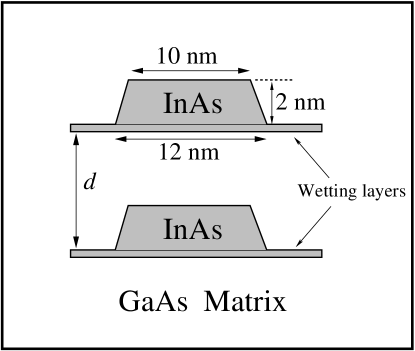
Figure 2: Geometry of the two vertically coupled quantum dot molecule. The inter-dot distance $d$ is measured from wetting layer to wetting layer.

II.2 Calculating the single-particle states

The single-particle electronic energy levels and wavefunctions are obtained by solving the Schrödinger equations in a pseudopotential scheme,

$$\left[-{1\over 2}\nabla^{2}+V_{\rm ps}({\bf r})\right]\psi_{i}({\bf r})=\epsilon_{i}\;\psi_{i}({\bf r})\;,$$ (1)

where the total electron-ion potential $V_{\rm ps}({\bf r})$ is a superposition of local, screened atomic pseudopotentials $v_{\alpha}({\bf r})$, i.e. $V_{\rm ps}({\bf r})=\sum_{n,\alpha}v_{\alpha}({\bf r}-{\bf R}_{n,\alpha})$. The pseudopotentials used for InAs/GaAs are identical to those used in Ref. Williamson et al., 2000 and were tested for different systems.Williamson et al. (2000); Bester et al. (2004); He et al. (2004) We ignored spin-orbit coupling in the InAs/GaAs quantum dots, since it is extremely small for electrons treated here (but not for holes which we do not discuss in the present work). Without spin-orbit coupling, the states of two electrons are either pure singlet, or pure triplet. However, if a spin-orbit coupling is introduced, the singlet state would mix with triplet state.

Equation (1) is solved using the “linear combination of Bloch bands” (LCBB) method,Wang and Zunger (1999) where the wavefunctions $\psi_{i}$ are expanded as,

$$\psi_{i}({\bf r})=\sum_{n,{\bf k}}\sum_{\lambda}C_{n,{\bf k}}^{(\lambda)}\;\phi_{n,{\bf k},\tensor{\epsilon}}^{(\lambda)}({\bf r})\;.$$ (2)

In the above equation, $\{\phi_{n,k,\tensor{\epsilon}}^{(\lambda)}({\bf r})\}$ are the bulk Bloch orbitals of band index $n$ and wave vector ${\bf k}$ of material $\lambda$ (= InAs, GaAs), strained uniformly to strain $\tensor{\epsilon}$. The dependence of the basis functions on strain makes them variationally efficient. (Note that the potential $V_{\rm ps}({\bf r})$ itself also has the inhomogeneous strain dependence through the atomic position ${\bf R}_{n,\alpha}$.) We use for the basis set $\tensor{\epsilon}=0$ for the (unstrained) GaAs matrix material, and an average $\tensor{\epsilon}$ value from VFF for the strained dot material (InAs). For the InAs/GaAs system, we use $n=2$ (including spin) for electron states on a 6$\times$6$\times$28 k-mesh. A single dot with the geometry of Fig.2 (base=12 nm and height=2 nm) has three bound electron states ($s$, $p_{1}$, and $p_{2}$) and more than 10 bound hole states. The lowest exciton transition in the single dot occurs at energy 1.09 eV. For the dot molecule the resulting single-particle states are, in order of increasing energy, the singly degenerated $\sigma_{g}$ and $\sigma_{u}$, (bonding and antibonding combination of the s-like single-dot orbitals), and the doubly (nearly) degenerated $\pi_{u}$ and $\pi_{g}$, originating from doubly (nearly) degenerate “p” orbitals (split by a few meV) in a single dot. Here, we use the symbols $g$ and $u$ to denote symmetric and anti-symmetric states, even though in our case the single-particle wavefunction are actually asymmetric.He et al. (2005) We define the difference between the respective dot molecule eigenvalues as $\Delta_{\sigma}=\epsilon(\sigma_{u})-\epsilon(\sigma_{g})$ and $\Delta_{\pi}=\epsilon(\pi_{g})-\epsilon(\pi_{u})$.

II.3 Calculating the many-particle states

The Hamiltonian of interacting electrons can be written as,

$$H=\sum_{i\sigma}\epsilon_{i}\psi^{{\dagger}}_{i\sigma}\psi_{i\sigma}+{1\over 2}\sum_{ijkl}\sum_{\sigma,\sigma^{\prime}}\Gamma^{ij}_{kl}\;\psi^{{\dagger}}_{i\sigma}\,\psi^{{\dagger}}_{j\sigma^{\prime}}\,\psi_{k\sigma^{\prime}}\,\psi_{l\sigma}\,,$$ (3)

where, $\psi_{i}$= $\sigma_{u}$, $\sigma_{g}$, $\pi_{u}$, $\pi_{g}$ are the single-particle energy levels of the $i$-th molecular orbital, while $\sigma$, $\sigma^{\prime}$=1, 2 are spin indices. The $\Gamma^{ij}_{kl}$ are the Coulomb integrals between molecular orbitals $\psi_{i}$, $\psi_{j}$, $\psi_{k}$ and $\psi_{l}$,

$$\Gamma^{ij}_{kl}=\int\int d{\bf r}d{\bf r^{\prime}}\;{\psi^{*}_{i}({\bf r})\psi^{*}_{j}({\bf r^{\prime}})\psi_{k}({\bf r^{\prime}})\psi_{l}({\bf r})\over\epsilon({\bf r}-\bf{r^{\prime}})|{\bf r}-{\bf r^{\prime}}|}\,.$$ (4)

The $J_{ij}=\Gamma^{ij}_{ji}$ and $K_{ij}=\Gamma^{ij}_{ij}$ are diagonal Coulomb and exchange integrals respectively. The remaining terms are called off-diagonal or scattering terms. All Coulomb integrals are calculated numerically from atomistic wavefunctions. Franceschetti et al. (1999) We use a phenomenological, position-dependent dielectric function $\epsilon({\bf r}-\bf{r^{\prime}})$ to screen the electron-electron interaction.Franceschetti et al. (1999)

We solve the many-body problem of Eq.(3) via the CI method, by expanding the $N$-electron wavefunction in a set of Slater determinants, $|\Phi_{e_{1},e_{2},\cdots,e_{N}}\rangle=\phi^{{\dagger}}_{e_{1}}\phi^{{\dagger}}_{e_{2}}\cdots\phi^{{\dagger}}_{e_{N}}|\Phi_{0}\rangle$, where $\phi^{{\dagger}}_{e_{i}}$ creates an electron in the state $e_{i}$ . The $\nu$-th many-particle wavefunction is then the linear combinations of the determinants,

$$|\Psi_{\nu}\rangle=\sum_{e_{1},e_{2},\cdots,e_{N}}A_{\nu}(e_{1},e_{2},\cdots,e_{N})\;|\Phi_{e_{1},e_{2},\cdots,e_{N}}\rangle\;.$$ (5)

In this paper, we only discuss the two-electron problem, i.e. $N$=2. Our calculations include all possible Slater determinants for the six single-particle levels.

II.4 Calculating pair correlation functions and degree of entanglement

We calculate in addition to the energy spectrum and the singlet-triplet splitting $J_{S-T}$ also the pair correlation functions and the degrees of entanglement (DOE). The pair correlation function $P_{\nu}({\bf r},{\bf r^{\prime}})$ for an $N$-particle system is defined as the probability of finding an electron at ${\bf r^{\prime}}$, given that the other electron is at ${\bf r}$, i.e.,

$$P_{\nu}({\bf r},{\bf r^{\prime}})=\int d{\bf r}_{3}\cdots d{\bf r}_{N}|\Psi_{\nu}({\bf r},{\bf r^{\prime}},{\bf r}_{3},\cdots,{\bf r}_{N})|^{2}\;,$$ (6)

where, $\Psi_{\nu}({\bf r}_{1},\cdots,{\bf r}_{N})$ is the $N$-particle wavefunction of state $\nu$. For two electrons, the pair correlation function is just $P_{\nu}({\bf r},{\bf r^{\prime}})=|\Psi_{\nu}({\bf r},{\bf r^{\prime}})|^{2}$.

The degree of entanglement (DOE) is one of the most important quantities for successful quantum gate operations. For distinguishable particles such as electron and hole, the DOE can be calculated from Von Neumann-entropy formulation. Nielsen and Chuang (2000); Bennett et al. (1996a, b); Wehrl (1978) However, for indistinguishable particles, there are some subtleties Schliemann et al. (2001a); Pas̆kauskas and You (2001); Li et al. (2001); Zanardi (2002); Shi (2003); Wiseman and Vaccaro (2003); Ghirardi and Marinatto (2004) for defining the DOE since it is impossible to separate the two identical particles. Recently, a quantum correlation function Schliemann et al. (2001a) has been proposed for indistinguishable particles using the Slater decompositions. Yang (1962) We adapt this quantum correlation function to define the DOE for indistinguishable fermions as,

$$\mathcal{S}=-\sum_{u}z_{i}^{2}\;{\rm log}_{2}\,z_{i}^{2}\;,$$ (7)

where, $z_{i}$ are Slater decomposition coefficients. The details of deriving Eq. (7) are given is Appendix A. We also show in Appendix A that the DOE measure Eq.(7) reduces to the usual Von Neumann-entropy formulation when the two-electrons are far from each other.

III results

Figure 3 shows the bonding-antibonding splitting $\Delta_{\sigma}(d)$ between the molecular orbitals vs inter-dot separation $d$ measured from one wetting layer to the other, showing also the value $\delta_{sp}=\epsilon_{p}-\epsilon_{s}$ of the splitting between the p and s orbital energies of a single dot (i.e. $d\rightarrow\infty$). The bonding-antibonding splitting decays approximately exponentially as $\Delta_{\sigma}=2.87\exp(-d/1.15)$ eV between $d\sim$4 - 8 nm. The result of bonding-antibonding splitting includes two competing effects. On one hand, large interdot distance $d$ reduces the coupling between the two dots; on the other hand, the strain between the dots is also reduced, leading to a lower tunneling barrier, thus increases coupling. The local maximum of $\Delta_{\sigma}$ at $d$=8.5 nm is a consequence of the this competition. Recent experiments Ota et al. (2003, 2004) show the bonding-antibonding splitting of about 4 meV at $d$=11.5 nm for vertically coupled InAs/GaAs quantum dots molecules, of similar magnitude as the value obtained here($\sim$ 1 meV), considering that the measured dot molecule is larger (height/base= 4 nm/40 nm rather than 2 nm/12 nm in our calculations) and possibly asymmetric. We also give in Fig. 3 the interelectronic Coulomb energy $J_{C}$ of a single-dot s orbital. We define strong coupling region as $\Delta_{\sigma}$ $\approx$ $\delta_{sp}$, and weak coupling region $\Delta_{\sigma}$ $\ll$ $\delta_{sp}$. We see in Fig. 3 strong coupling for $d\leq$ 4 nm, and weak coupling for $d\geq$ 5 nm. In the weak coupling region, the $\pi$ levels are well above the $\sigma$ levels. We also define “strong confinement” as $\delta_{sp}>J_{C}$, and weak confinement as the reverse inequality. Figure 3 shows that our dot is in the strong-confinement regime. In contrast, electrostatic dot Ashoori et al. (1992); Johnson et al. (1992); Tarucha et al. (1996) are in the weak confinement regime.

We next discuss the two-electron states in the QDMs and examine several different approximations which we call Levels 1 - 4, by comparing the properties of the ground states, the singlet-triplet energy separation $J_{S-T}$ and the pair correlation functions as well as the degree of entanglement for each state. Starting from our most complete model (Level 1) and simplifying it in successive steps, we reduce the sophistication with which interelectronic correlation is described and show how these previously practiced approximations lead to different values of $J_{S-T}$ (including its sign reversal), and different degree of entanglement. This methodology provides insight into the electronic features which control singlet-triplet splitting and electron-electron entanglement in dot molecules.

III.1 Level-1 theory: all-bound-state configuration interaction

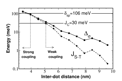
Figure 3: The bonding-antibonding splitting $\Delta_{\sigma}=\epsilon(\sigma_{g})-\epsilon(\sigma_{u})$ (solid line) and singlet-triplet splitting $J_{S-T}=E(^{3}\Sigma)-E(^{1}\Sigma_{g}^{(a)})$ (dashed line) vs inter-dot distance $d$. We also show the single-dot s, p orbitals splitting $\delta_{sp}=e_{s}-e_{p}$ and the s orbital Coulomb interaction $J_{C}$. We define “strong coupling” by $\Delta_{\sigma}\sim\delta_{sp}$ ($<$ 4 nm) and “weak coupling”, $\Delta_{\sigma}\ll\delta_{sp}$ ($>$ 5 nm).

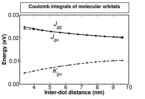
Figure 4: Selected Coulomb integrals for molecular orbitals. $J_{gg}$ is the self-Coulomb energy of the $\sigma_{g}$ orbital and $J_{gu}$ is the Coulomb energy between $\sigma_{g}$ and $\sigma_{u}$ orbitals, while $K_{gu}$ is the exchange energy between $\sigma_{g}$ and $\sigma_{u}$ orbitals.

We first study the two-electron states by solving the CI Eq. (5), using all confined molecular orbitals $\sigma_{g}$, $\sigma_{u}$ and $\pi_{g}$, $\pi_{u}$, to construct the Slater determinants. This gives a total of 66 Slater determinants. The continuum states are far above the bound-state, and are thus not included in the CI basis. Figure 4 shows some important matrix elements, including $J_{gg}$ (Coulomb energy of $\sigma_{g}$ MO), $J_{gu}$ (Coulomb energy between $\sigma_{g}$ and $\sigma_{u}$), and $K_{gu}$ (exchange energy between $\sigma_{g}$ and $\sigma_{u}$). The Coulomb energy between $\sigma_{u}$ MO, $J_{uu}$ is nearly identical to $J_{gg}$ and therefore is not plotted. Diagonalizing the all-bound-state CI problem gives the two-particle states, shown in Fig.5a. We show all six $\Sigma$ states (where both electrons occupy the $\sigma$ states) and the two lowest three-fold degenerate ${}^{3}\Pi_{u}$ states (where one electron occupies the $\sigma_{g}$ and one occupies one of the $\pi$ levels). We observe that:

(a) The ground-state is singlet ${}^{1}\Sigma_{g}^{(a)}$ for all dot-dot distances. However, the character of the state is very different at different inter-dot separation $d$, which can be analyzed by the isospin of the state, Palacios and Hawrylak (1995) defined as the difference in the number of electrons occupying the bonding ($N_{B}$) and antibonding ($N_{AB}$) states in a given CI state, i.e. $I_{z}=(N_{B}-N_{AB})/2$, where $N_{B}$ and $N_{AB}$ are obtained from Eq.(5). As shown in Fig.6, $I_{z}(d)$ of the ${}^{1}\Sigma_{g}^{(a)}$ state is very different at different inter-dot distances: At small inter-dot distance, the dominant configuration of the ground state is $|\sigma_{g}^{\uparrow},\sigma_{g}^{\downarrow\rangle}$ (both electrons occupy bonding state and $N_{B}$=2), and $I_{z}$$\sim$1. However, in the weak coupling region, there is significant mixing of bonding $\sigma_{g}$ and anti-bonding states $\sigma_{u}$, and $I_{z}$ is smaller than 1, e.g $I_{z}$$\sim$ 0.2 at $d$= 9.5 nm. At infinite separation, where the bonding and antibonding states are degenerate, one expects $I_{z}$$\rightarrow$ 0.

(b) Next to the ground state, we find in Fig.5a the three-fold degenerate triplet states ${}^{3}\Sigma_{u}$, with $S_{z}$=1, -1 and 0. In the absence of spin-orbit coupling, triplet states will not couple to singlet states. If we include spin-orbit coupling, the triplet may mix with the singlet state, and the degeneracy will be lifted. At large inter-dot distances, the ground state singlet ${}^{1}\Sigma_{g}^{(a)}$ and triplet states ${}^{3}\Sigma_{u}$ are degenerate. The splitting of total CI energy between ground state singlet and triplet $J_{S-T}=E(^{3}\Sigma)-E(^{1}\Sigma_{g})$ is plotted in Fig.3 on a logarithmic scale. As we can see, $J_{S-T}$ also decays approximately exponentially between 4 and 8 nm, and can be fitted as $J_{S-T}=5.28\exp(-d/0.965)$ eV. The decay length of 0.965 nm is shorter than the decay length 1.15 nm of $\Delta_{\sigma}$. At small inter-dot separations, $J_{S-T}\sim\Delta_{\sigma}$ in Fig.3, as expected from a simple Heitler-London model. Burkard et al. (1999)

(c) The two excited singlet states originating from the occupation of $\sigma_{u}$ anti-bonding states, ${}^{1}\Sigma_{u}$ and ${}^{1}\Sigma_{g}^{(b)}$ are further above the ${}^{3}\Sigma_{u}$ state.

(d) The lowest ${}^{3}\Pi_{u}$ states are all triplet states. They are energetically very close to each other since we have two nearly degenerate $\pi_{u}$ MO states. In the weak coupling region, the $\Pi_{u}$ states are well above the $\Sigma$ states, as a consequence of large single-particle energy difference $\epsilon(\pi_{u})-\epsilon(\sigma_{u})$. However, the $\Pi_{u}$, and ${}^{1}\Sigma_{g}^{(b)}$ cross at about 4.5 nm, where the single-particle MO level $\pi_{u}$ is still much higher than $\sigma_{u}$. In this case, the Coulomb correlations have to be taken into account.

In the following sections, we enquire as to possible, popularly practiced simplifications over the all-bound-states CI treatment.

III.2 Level-2 theory: reduced CI in the molecular basis

In Level-2 theory, we will reduce the full 66$\times$66 CI problem of Level-1 to one that includes only the $\sigma_{g}$ and $\sigma_{u}$ basis, giving a 6$\times$6 CI problem. The six many-body basis states are shown in Fig.1a, $|a\rangle$=$|\sigma_{g}^{\uparrow},\sigma_{u}^{\uparrow}\rangle$, $|b\rangle$=$|\sigma_{g}^{\downarrow},\sigma_{u}^{\downarrow}\rangle$, $|c\rangle$=$|\sigma_{g}^{\uparrow},\sigma_{u}^{\downarrow}\rangle$, $|d\rangle$=$|\sigma_{g}^{\downarrow},\sigma_{u}^{\uparrow}\rangle$, $|e\rangle$=$|\sigma_{g}^{\uparrow},\sigma_{g}^{\downarrow}\rangle$, $|f\rangle$=$|\sigma_{u}^{\uparrow},\sigma_{u}^{\downarrow}\rangle$. In this basis set, the CI problem is reduced to a 6$\times$6 matrix eigenvalue equation,

$$\scriptsize H=\left(\begin{array}[]{cccccc}\epsilon_{g}+\epsilon_{u}+J_{gu}-K_{gu}&0&0&0&0&0\\ 0&\epsilon_{g}+\epsilon_{u}+J_{gu}-K_{gu}&0&0&0&0\\ 0&0&\epsilon_{g}+\epsilon_{u}+J_{gu}&-K_{gu}&-\Gamma^{gu}_{gg}&-\Gamma^{gu}_{uu}\\ 0&0&-K_{gu}&\epsilon_{g}+\epsilon_{u}+J_{gu}&\Gamma^{gu}_{gg}&\Gamma^{gu}_{uu}\\ 0&0&-\Gamma^{gg}_{gu}&\Gamma^{gg}_{gu}&2\epsilon_{g}+J_{gg}&\Gamma^{gg}_{uu}\\ 0&0&-\Gamma^{uu}_{gu}&\Gamma^{uu}_{gu}&\Gamma^{uu}_{gg}&2\epsilon_{u}+J_{uu}\end{array}\right)\normalsize$$ (8)

where, $\epsilon_{g}$ and $\epsilon_{u}$ are the single-particle energy levels for the MO’s $|\sigma_{g}\rangle$ and $|\sigma_{u}\rangle$, respectively. In the absence of spin-orbit coupling, the triplet states $|a\rangle$ and $|b\rangle$ are not coupled to any other states, as required by the total spin conservation, and thus they are already eigenstates. The rest of the matrix can be solved using the integrals calculated from Eq.(4). The results of the 6$\times$6 problem were compared (not shown) to the all-bound-state CI results: We find that the $\Sigma$ states of Level-2 theory are very close to those of the all-bound-state CI calculations, indicating a small coupling between $\sigma$ and $\pi$ orbitals in the strong confinement region. We thus do not show graphically the results of Level-2. However, since we use only $\sigma$ orbitals, the $\Pi$ states of Level-1 (Fig.5a) are absent in Level-2 theory. Especially, the important feature of crossover between $\Sigma$ and $\Pi_{u}$ states at 4 and 4.5 nm is missing.

III.3 Level-3 theory: single-configuration in the molecular basis

As is well known, mean-field-like treatments such as RHF and LSD usually give incorrect dissociation behavior of molecules, as the correlation effects are not adequately treated. Given that RHF and LSD are widely used in studying QMDs, Tamura (1998); Nagaraja et al. (1999); Partoens and Peeters (2000) it is important to understand under which circumstance the methods will succeed and under which circumstance they will fail in describing the few-electron states in a QDM. In level-3 theory, we thus mimic the mean-field theory by further ignoring the off-diagonal Coulomb integrals in Eq.(8) of Level-2 theory, i.e., we assume $\Gamma^{gu}_{uu}$= $\Gamma^{gu}_{gg}$ =$\Gamma^{uu}_{gg}$=0. This approximation is equivalent to ignoring the coupling between different configurations, and is thus called “single-configuration” (SC) approximation. At the SC level, we have very simple analytical solutions of the two-electron states,

$$E(^{1}\Sigma_{g}^{(a)}) = 2\epsilon_{g}+J_{gg};\quad\quad\quad\quad\quad\quad\;\;|^{1}\Sigma_{g}^{(a)}\rangle=|e\rangle\;\;,$$ (9)

$$E(^{3}\Sigma_{u}) = (\epsilon_{g}+\epsilon_{u})+J_{gu}-K_{gu};\;\left\{\begin{array}[]{l}|^{3}_{+}\Sigma_{u}\rangle=|a\rangle\;,\\ |^{3}_{-}\Sigma_{u}\rangle=|b\rangle\;,\\ |^{3}_{0}\Sigma_{u}\rangle=|c\rangle-|d\rangle\;,\end{array}\right.$$ (13)

$$E(^{1}\Sigma_{u}) = (\epsilon_{g}+\epsilon_{u})+J_{gu}+K_{gu};\quad\;|^{1}\Sigma_{u}\rangle=|c\rangle+|d\rangle\;\;,$$ (14)

$$E(^{1}\Sigma_{g}^{(b)}) = 2\epsilon_{u}+J_{uu};\quad\quad\quad\quad\quad\quad\;\;|^{1}\Sigma_{g}^{(b)}\rangle=|f\rangle\;\;.$$ (15)

The energies are plotted in Fig.5b. When comparing the $\Sigma$ states of the SC approach to the all-bound-state CI results in Fig.5a, we find good agreement in the strong coupling region for $d\leq$ 5 nm (see Fig.3). However, the SC approximation fails qualitatively at larger inter-dot separations in two aspects: (i) The order of singlet state ${}^{1}\Sigma_{g}^{(a)}$ and triplet state ${}^{3}\Sigma_{u}$ is reversed (see Fig. 5b,c). (ii) The ${}^{1}\Sigma_{g}^{(a)}$ and ${}^{3}\Sigma_{u}$ states fail to be degenerate at large interdot separation. This lack of degeneracy is also observed for ${}^{1}\Sigma_{g}^{(b)}$ and ${}^{1}\Sigma_{u}$. These failures are due to the absence of correlations in the SC approximation. Indeed as shown in Fig.6, the accurate Level-1 ground state singlet has considerable mixing of anti-bonding states, i.e. $I_{z}\rightarrow 0$ at large $d$. However, in the SC approximation both electrons are forced to occupy the $\sigma_{g}$ orbital in the lowest singlet state ${}^{1}\Sigma_{g}^{(a)}$ as a consequence of the lack of the coupling between the configuration $|e\rangle$ of Fig.1a and other configurations. As a result, in Level-3 theory, the isospins are forced to be $I_{z}$=1 for ${}^{1}\Sigma_{g}^{(a)}$ at all inter-dot distances $d$, which pushes the singlet energy higher than the triplet.

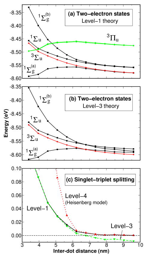
Figure 5: (Color online) (a) Two-electron states calculated from CI using all confined MO from LCBB (Level-1), including the singlet ${}^{1}\Sigma_{g}^{(a)}$, ${}^{1}\Sigma_{u}$, ${}^{1}\Sigma_{g}^{(b)}$ states and the 3-fold degenerated triplet states ${}^{3}\Sigma_{u}$ as well as two 3-fold degenerated triplet states ${}^{3}\Pi_{u}$. (b) Two electron states calculated from the single-configuration approximation (Level-3). (c) Comparison of the singlet-triplet splitting calculated from Levels 1, 3 and 4 theories.

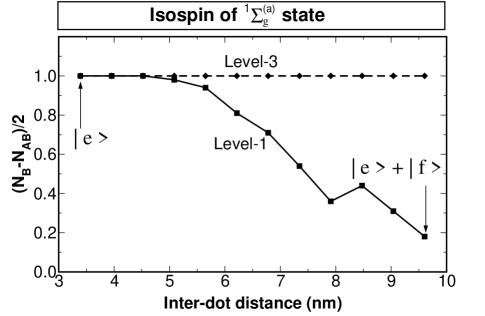
Figure 6: Isospin, defined as the difference in the number of electrons occupying the bonding ($N_{B}$) and antibonding ($N_{AB}$) states, of the ${}^{1}\Sigma_{g}^{(a)}$ state in Level-1 and Level-3 theories.

III.4 Level-4 theory: Hubbard model and Heisenberg model in a dot-centered basis

The Hubbard model and the Heisenberg model are often used Loss and DiVincenzo (1998) to analyze entanglement and gate operations for two spins qbits in a QDM. Here, we analyze the extent to which such approaches can correctly capture the qualitative physics given by more sophisticated models. Furthermore, by doing so, we obtain the parameters of the models from realistic calculations.

III.4.1 Transforming the states to a dot-centered basis

Unlike the Level 1 - 3 theories, the Hubbard and the Heisenberg models are written in a dot-centered basis as shown in Fig.1b, rather than in the molecular basis of Fig.1a. In a dot-centered basis, the Hamiltonian of Eq.(3) can be rewritten as,

$$H=\sum_{\eta_{1},\eta_{2}}\sum_{\sigma}(e_{\eta_{1}}\delta_{\eta_{1}\eta_{2}}+t_{\eta_{1}\eta_{2}})\chi^{{\dagger}}_{\eta_{1},\sigma}\,\chi_{\eta_{2}\sigma}+{1\over 2}\sum_{\eta_{1},\cdots,\eta_{4}}\sum_{\sigma,\sigma^{\prime}}\widetilde{\Gamma}^{\eta_{1},\eta_{2}}_{\eta_{3},\eta_{4}}\;\chi^{{\dagger}}_{\eta_{1},\sigma}\,\chi^{{\dagger}}_{\eta_{2},\sigma^{\prime}}\,\chi_{\eta_{3},\sigma^{\prime}}\,\chi_{\eta_{4},\sigma}\,,$$ (16)

where, $\eta=(l,p)$ and $\chi^{{\dagger}}_{\eta,\sigma}$ creates an electron in the $l$=(s, p, $\cdots$) orbital on the $p$=(T, B) dot with spin $\sigma$ that has single-particle energy $e_{\eta}$. Here, $t_{\eta_{1}\eta_{2}}$ is the coupling between the $\eta_{1}$ and $\eta_{2}$ orbitals, and $\widetilde{\Gamma}^{\eta_{1},\eta_{2}}_{\eta_{3},\eta_{4}}$ is the Coulomb integral of single-dot orbitals $\chi_{\eta_{1}}$, $\chi_{\eta_{2}}$, $\chi_{\eta_{3}}$ and $\chi_{\eta_{4}}$.

We wish to construct a Hubbard Hamiltonian whose parameters are taken from the fully atomistic single-particle theory. To obtain such parameters in Eq.(16) including $e_{\eta}$, $t_{\eta_{1}\eta_{2}}$ and $\widetilde{\Gamma}^{\eta_{1},\eta_{2}}_{\eta_{3},\eta_{4}}$, we resort to a Wannier-like transformation, which transform the “molecular” orbitals (Fig.1a) into single-dot “atomic” orbitals (Fig.1b). The latter dot-centered orbitals are obtained from a unitary rotation of the molecular orbitals $\psi_{i}$, i.e,

$$\chi_{\eta}=\sum_{i=1}\mathcal{U}_{\eta\,,i}\,\psi_{i}\;,$$ (17)

where, $\psi_{i}$ is the $i$-th molecular orbitals, $\chi_{\eta}$ is the single dot-centered orbitals, and $\mathcal{U}$ are unitary matrices, i.e. $\mathcal{U}^{{\dagger}}\mathcal{U}=I$. We chose the unitary matrices that maximize the total orbital self-Coulomb energy. The procedure of finding these unitary matrices is described in detail in Appendix B. The dot-centered orbitals constructed this way are approximately invariant to the change of coupling between the dots.Edmiston and Ruedenberg (1963) Once we have the $\mathcal{U}$ matrices, we can obtain all the parameters in Eq.(16) by transforming them from the molecular basis. The Coulomb integrals in the new basis set are given by Eq. (37), while other quantities including the effective single-particle levels $e_{\eta}$ for the $\eta$-th dot-centered orbital, and the coupling between the $\eta_{1}$-th and $\eta_{2}$-th orbitals $t_{\eta_{1}\eta_{2}}$ can be obtained from,

$$e_{\eta} = \langle\chi_{\eta}|\hat{T}|\chi_{\eta}\rangle=\sum_{i}\mathcal{U}^{*}_{\eta\,,i}\,\mathcal{U}_{\eta\,,i}\,\epsilon_{i}\;,$$ (18)

$$t_{\eta_{1}\eta_{2}} = \langle\chi_{\eta_{1}}|\hat{T}|\chi_{\eta_{2}}\rangle=\sum_{i}\mathcal{U}^{*}_{\eta_{1},\,i}\,U_{\eta_{2},\,i}\,\epsilon_{i}\;,$$ (19)

where $\epsilon_{i}$ is the single-particle level of the $i$-th molecular orbital, and $\hat{T}$ is kinetic energy operator. Using the transformation of Eq.(18), Eq.(19) and Eq.(37), we calculate all parameters of Eq.(16). Figure 7a, shows the effective single-dot energy of the “s” orbitals obtained in the Wannier representation for both top and bottom dots. We see that the effective single-dot energy levels increase rapidly for small $d$. Furthermore the energy levels for the top and bottom orbitals are split due to the strain asymmetry between the two dots. We compute the Coulomb energies $J_{\rm TT}$, $J_{\rm BB}$ of the “s” orbitals on both top and bottom dots, and the inter-dot Coulomb and exchange energies $J_{\rm TB}$ and $K_{\rm TB}$ and plot these quantities in Fig. 7b. Since $J_{\rm TT}$ and $J_{\rm BB}$ are very similar, we plot only $J_{\rm TT}$. As we can see, the Coulomb energies of the dot-centered orbitals are very close to the Coulomb energy of the s orbitals of a isolated single dot (dashed line). The inter-dot Coulomb energy $J_{\rm TB}$ has comparable amplitude to $J_{\rm TT}$ and decays slowly with distance, and remain very significant, even at large separations. However, the exchange energy between the orbitals localized on top dot and bottom dot $K_{\rm TB}$ is extremely small even when the dots are very close.

III.4.2 “First-principles” Hubbard model and Heisenberg model: Level-4

In level-4 approximation, we use only the “s” orbital in each dot. Figure 1b shows all possible many-body basis functions of two electrons, where top and bottom dots are denoted by “T” and “B” respectively. The Hamiltonian in this basis set is,

$$\scriptsize H=\left(\begin{array}[]{cccccc}e_{\rm T}+e_{\rm B}+J_{\rm TB}-K_{\rm TB}&0&0&0&0&0\\ 0&e_{\rm T}+e_{\rm B}+J_{\rm TB}-K_{\rm TB}&0&0&0&0\\ 0&0&e_{\rm T}+e_{\rm B}+J_{\rm TB}&-K_{\rm TB}&t-\widetilde{\Gamma}^{\rm TB}_{\rm BB}&t-\widetilde{\Gamma}^{\rm TB}_{\rm TT}\\ 0&0&-K_{\rm TB}&e_{\rm T}+e_{\rm B}+J_{\rm TB}&-t+\widetilde{\Gamma}^{\rm TB}_{\rm BB}&-t+\widetilde{\Gamma}^{\rm TB}_{\rm TT}\\ 0&0&t-\widetilde{\Gamma}^{\rm BB}_{\rm TB}&-t+\widetilde{\Gamma}^{\rm BB}_{\rm TB}&2e_{\rm B}+J_{\rm BB}&0\\ 0&0&t-\widetilde{\Gamma}^{\rm TT}_{\rm TB}&-t+\widetilde{\Gamma}^{\rm TT}_{\rm TB}&0&2e_{\rm T}+J_{\rm TT}\end{array}\right)\;.\normalsize$$ (20)

where $t=t_{TB}$ and to simplify the notation, we ignore the orbital index “s”. If we keep all the matrix elements, the description using the molecular basis of Fig. 1a and the dot localized basis of Fig. 1b are equivalent, since they are connected by unitary transformations. We now simplify Eq.(20) by ignoring the off-diagonal Coulomb integrals. The resulting Hamiltonian is the single-band Hubbard model. Unlike Level-3 theory, in this case, ignoring off-diagonal Coulomb integrals (but keeping hopping) can still give qualitatively correct results, due to the fact that off-diagonal Coulomb integrals such as $\widetilde{\Gamma}^{\rm BB}_{\rm TB}\ll t$, and the correlation is mainly carried by inter-dot hopping $t$. We can further simplify the model by assuming $e_{\rm T}=e_{\rm B}=\epsilon$; $J_{\rm TT}=J_{\rm BB}=U$; and let $J_{\rm TB}=V$, $K_{\rm TB}=K$. We can then solve the simplified eigenvalue equation analytically. The eigenvalues of the above Hamiltonian are (in order of increasing energy):
1. Ground state singlet ${}^{1}\Sigma_{g}^{(a)}$

$$E=2\epsilon+{1\over 2}[U+V+K-\sqrt{16t^{2}+(U-V-K)^{2}}]$$ (21)

2. Triplet states (three-fold degenerate) ${}^{3}\Sigma_{u}$

$$E=2\epsilon+V-K$$ (22)

3. Singlet ${}^{1}\Sigma_{u}$

$$E=2\epsilon+U$$ (23)

4. Singlet ${}^{1}\Sigma_{g}^{(b)}$

$$E=2\epsilon+{1\over 2}[U+V+K+\sqrt{16t^{2}+(U-V-K)^{2}}]$$ (24)

In the Hubbard limit where Coulomb energy $U\gg t$, the singlet-triplet splitting $J_{S-T}=E(^{3}\Sigma)-E(^{1}\Sigma_{g})\sim 4t^{2}/(U-V)$, which reduces the model to the Heisenberg model

$$H={4t^{2}\over U-V}\,\vec{S}_{T}\cdot\vec{S}_{B}\;,$$ (25)

where $\vec{S}_{T}$ and $\vec{S}_{B}$ are the spin vectors on the top and bottom dots. The Heisenberg model gives the correct order for singlet and triplet states. The singlet-triplet splitting $J_{S-T}=4t^{2}/(U-V)$ is plotted in Fig. 5c and compared to the results from all-bound-state CI calculations (Level-1), and single-configuration approximations (Level-3). As we can see, at $d>$ 6.5 nm, the agreement between the Heisenberg model with CI is good, but the Heisenberg model greatly overestimates $J_{S-T}$ at $d<$ 6 nm.

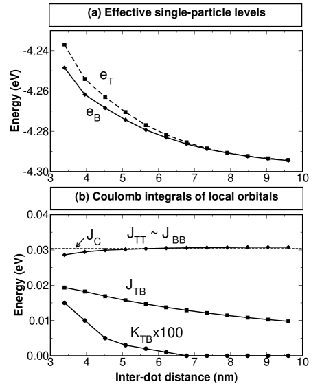
Figure 7: (a) Effective single-particle energy levels of s orbitals localized on the top ($e_{T}$) and bottom ($e_{B}$) dots. (b) Intra-dot Coulomb energy $J_{\rm TT}$, $J_{\rm BB}$, inter-dot Coulomb energy $J_{\rm TB}$ and inter-dot exchange energy $K_{\rm TB}$ (magnified by a factor 100). The dashed line gives the single-dot s orbital self-Coulomb energy $J_{C}$.

III.5 Comparison of pair correlation functions for Levels-1 to 4 theories

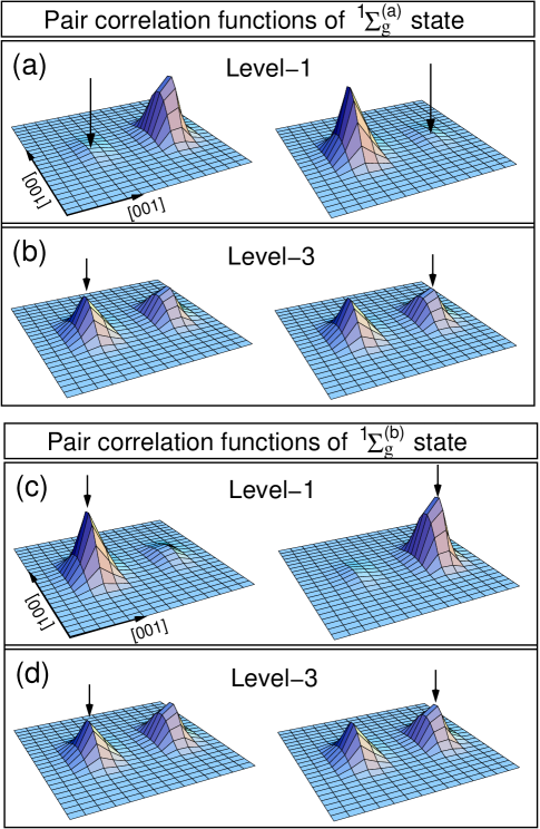
Figure 8: (Color online) Comparison of pair correlation functions calculated from (a) Level-1, (b) Level-3 theory for the ${}^{1}\Sigma_{g}^{(a)}$ state and (c) Level-1, (d) Level-3 theory for the ${}^{1}\Sigma_{g}^{(b)}$ state at $d\sim$ 7 nm. On the left hand side, the first electron is fixed at the center of the bottom dot, while on the right hand side, the first electon is fixed at the center of the top dot, as indicated by the arrows.

In the previous sections, we compared the energy levels of two-electron states in several levels of approximations to all-bound-state CI results (Level-1). We now provide further comparison of Levels 1-4 theories by analyzing the pair correlation functions and calculating the electron-electron entanglement at different levels of approximations.

In Fig. 8 we show the pair correlation functions of Eq.(6) for the ${}^{1}\Sigma_{g}^{(a)}$ and ${}^{1}\Sigma_{g}^{(b)}$ states at $d\sim$ 7 nm for Level-1 and Level-3 theories. The correlation functions give the probability of finding the second electron when the first electron is fixed at the position shown by the arrows at the center of the bottom dot (left hand side of Fig. 8) or the top dot (right hand side of Fig. 8). Level-1 and Level-2 theories give correlation-induced electron localization at large $d$: for the ${}^{1}\Sigma_{g}^{(a)}$ state, the two electrons are localized on different dots, while for the ${}^{1}\Sigma_{g}^{(b)}$ state, both electrons are localized on the same dot.He et al. (2005) In contrast, Level-3 theory shows delocalized states because of the lack of configuration mixing. This problem is shared by RHF and LSD approximations.

III.6 Comparison of the degree of entanglement for Levels 1-4 theories

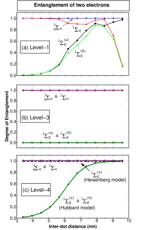
Figure 9: (Color online) Comparison of the DOE calculated from (a) Level-1; (b) Level-3 and (c) Level-4 theories for two-electron states. In panel (c), both the DOE of the Hubbard model (solid lines) and of the Heisenberg model for ${}^{1}\Sigma_{g}^{(a)}$ state (dashed line) are shown.

The DOE of the four “$\Sigma$” states are plotted in Fig.9 for Level-1, Level-3 and Level-4 theories; the DOE of Level-2 theory are virtually identical to those of Level-1 theory, and are therefore not plotted. We see that the Hubbard model has generally reasonable agreement with Level-1 theory while the DOE calculated from Level-3 and Level-4 (Heisenberg model) theories deviate significantly from the Level-1 theory, which is addressed below:

(i) The ${}^{1}\Sigma_{g}^{(a)}$ state: The Level-1 theory (Fig.9a), shows that the DOE of ${}^{1}\Sigma_{g}^{(a)}$ increases with $d$ and approaches 1 at large $d$. The Hubbard model of Level-4 theory (Fig.9c) gives qualitatively correct DOE for this state except for some details. However, Level-3 theory (Fig.9b) gives DOE $\mathcal{S}=0$ because the wavefunction of ${}^{1}\Sigma_{g}^{(a)}$ is a single Slater determinant $|e\rangle$ [see Eq.(9)]. For the same reason, the DOEs of the ${}^{1}\Sigma_{g}^{(a)}$ state in RHF and LSD approximations are also zero as a consequence of lack of correlation. In contrast, the Heisenberg model of Level-4 theory gives $\mathcal{S}(^{1}\Sigma_{g}^{(a)})=1$. This is because the Heisenberg model assumes that the both electrons are localized on different dots with zero double occupancy, and thus overestimates the DOE. Schliemann et al. (2001b); He et al. (2005)

(ii) The ${}^{1}\Sigma_{g}^{(b)}$ state: The Hubbard model gives the DOE of the ${}^{1}\Sigma_{g}^{(b)}$ state identical to that of ${}^{1}\Sigma_{g}^{(a)}$ state. This is different from the result of Level-1 theory, especially at large inter-dot separations. The difference comes from the assumption in the Hubbard model that the energy levels and wavefunctions on the top dot and on the bottom dot are identical while as discussed in Ref.He et al., 2005, the wavefunctions are actually asymmetric due to inhomogeneous strain in the real system. At $d>$ 8 nm, the ${}^{1}\Sigma_{g}^{(b)}$ state is the supposition of $|E\rangle$ and $|F\rangle$ configurations in the Hubbard model leading to $\mathcal{S}=1$, while in Level-1 theory, the two electrons are both localized on the top dots ($|F\rangle$) at $d>$ 9 nm,He et al. (2005) resulting in near zero entanglement. For the same reason discussed in (i), the Level-3 theory gives $\mathcal{S}(^{1}\Sigma_{g}^{(b)})=0$.

(iii) The ${}^{1}\Sigma_{u}$ state: Both the Level-3 theory and Hubbard model give $\mathcal{S}(^{1}\Sigma_{u})=1$. However, the $\mathcal{S}(^{1}\Sigma_{u})$ of the Level-1 theory has more features as the consequence of the asymmetry of the system. In contrast to the ${}^{1}\Sigma_{g}^{(b)}$ state, in the ${}^{1}\Sigma_{u}$ state, both electrons are localized on the bottom dot leading to near zero entanglement at $d>$ 9 nm.

(iv) The ${}^{3}\Sigma_{u}$ state: All levels of theories give very close results of DOE for ${}^{3}_{0}\Sigma_{u}$ state. Actually, in Level-1 theory, the DOE of ${}^{3}_{0}\Sigma_{u}$ state is only slightly larger than 1, indicating weak entanglement of the $\sigma$ and $\pi$ orbitals (the maximum entanglement one can get from the total of six orbitals is $\mathcal{S}_{\rm max}={\rm log}_{2}\,6$), while in all other theories (including the Level-2 theory) they are exactly 1 since these theories include only two $\sigma$ orbitals. The small coupling between $\sigma$ and $\pi$ orbitals is desirable for quantum computation, which requires the qbits states to be decoupled from other states.

IV summary

We have shown the energy spectrum, pair-correlation functions and degree of entanglement of two-electron states in self-assembled InAs/GaAs quantum dot molecules via all-bound-state configuration interaction calculations and compared these quantities in different levels of approximations. We find that the correlation between electrons in the top and bottom dot is crucial to get the qualitative correct results for both the singlet-triplet splitting and the degree of entanglement. The single-configuration approximation and similar theories such as RHF, LSD all suffer from lack of correlation and thus give incorrect ground state, singlet-triplet splitting $J_{S-T}$ and degree of entanglement. Highly simplified models, such as the Hubbard model gives qualitatively correct results for the ground state and $J_{S-T}$, while the Heisenberg model only give similar results at large $d$. These two models are written in the dot-centered basis, where the correlation between the top and bottom dots are carried by the single-particle tunneling. However, as a consequence of ignoring the asymmetry present in the real system, the degree of entanglement calculated from the Hubbard model deviates significantly from realistic atomic calculations. Moreover the Heisenberg model greatly overestimates the degree of entanglement of the ground state as a consequence of further ignoring the electron double occupancy in the dot molecule.

Appendix A Degree of entanglement for two electrons

The entanglement is characterized by the fact that the many-particle wavefunctions can not be factorized as a direct product of single-particle wavefunctions. An entangled system displays non-locality which is one of the properties that distinguishes it from classic systems. So far, the only well established theory of entanglement pertains to two distinguishable particles,Nielsen and Chuang (2000); Bennett et al. (1996b) (e.g. electron and hole). For a system made of two distinguishable particles $(A,B)$, the entanglement can be quantified by von Neumann entropy of the partial density matrix of either $A$ or $B$, Nielsen and Chuang (2000); Bennett et al. (1996a); Wehrl (1978)

$$\mathcal{S}(A,B)=-{\rm Tr}\;(\rho_{A}\;{\rm log}_{2}\,\rho_{A})=-{\rm Tr}\;(\rho_{B}\;{\rm log}_{2}\,\rho_{B})\;,$$ (26)

where $\mathcal{S}(A,B)$ is the DOE of the state. $\rho_{A}$ and $\rho_{B}$ are the reduced density matrices for subsystems $A$ and $B$. An alternative way to define the DOE for two distinguishable particles is through a Schmidt decomposition, where two-non-identical-particle wavefunctions are written in an bi-orthogonal basis,

$$\Psi(A,B)=\sum_{i}\lambda_{i}\;|i_{A}\rangle\otimes|i_{B}\rangle\,,$$ (27)

with $\lambda_{i}\geq 0$ and $\sum_{i}\lambda_{i}^{2}=1$. The number of nonzero $\lambda_{i}$ is called the Schmidt rank. For a pure state $\Psi(A,B)$ of the composite system $(A,B)$, we have,

$$\rho_{A} = \sum_{i}\lambda_{i}^{2}\;|i_{A}\rangle\langle i_{A}|$$

$$\rho_{B} = \sum_{i}\lambda_{i}^{2}\;|i_{B}\rangle\langle i_{B}|\,.$$ (28)

It is easy to show from Eq. 26 that the DOE for the two distinguishable particles is,

$$\mathcal{S}(A,B)=-\sum_{i}\lambda_{i}^{2}\;{\rm log}_{2}\,\lambda_{i}^{2}\;.$$ (29)

We see from Eq.(27) that when and only when the Schmidt rank equals 1, the two-particle wavefunction can be written as a direct product of two single-particle wavefunctions. In this case, we have $\lambda=1$, and $\mathcal{S}(A,B)=0$ from Eq.(29).

A direct generalization of DOE of Eq.(29) for two identical particles is problematic. Indeed, there is no general way to define the subsystem $A$ and $B$ for two identical particles. More seriously, since two-particle wavefunctions for identical particles are non-factorable due to their built-in symmetry, one may tend to believe that all two identical fermions (or Bosons) are in entangled Bell state.Nielsen and Chuang (2000) However, inconsistency comes up in the limiting cases. For example, suppose that two electrons are localized on each of the two sites $A$ and $B$ that are far apart, where the two electrons can be treated as distinguishable particles by assigning $A$ and $B$ to each electron, respectively. A pure state $\Psi$ that has the spin up for $A$ electron and spin down for $B$ electron is $\Psi({\bf x}_{1},{\bf x}_{2})=1/\sqrt{2}[\phi_{A\uparrow}({\bf x}_{1})\phi_{B\downarrow}({\bf x}_{2})-\phi_{A\uparrow}({\bf x}_{2})\phi_{B\downarrow}({\bf x}_{1})]$. At first sight, because of the anti-symmetrization, it would seem that the two electron states can not be written as a direct product of two single particle wavefunctions, so this state is maximally entangled. However, when the overlap between two wavefunctions is negligible, we can treat these two particles as if they were distinguishable particles and ignore the anti-symmetrization without any physical effect, i.e. $\Psi({\bf x}_{1},{\bf x}_{2})=\phi_{A\uparrow}({\bf x}_{1})\phi_{B\downarrow}({\bf x}_{2})$. In this case, apparently the two electrons are unentangled. More intriguingly, in quantum theory, all fermions have to be anti-symmetrized even for non-identical particles, which does not mean they are entangled.

To solve this obvious inconsistency, alternative measures of the DOE of two fermions have been proposed and discussed recently,Schliemann et al. (2001a); Pas̆kauskas and You (2001); Li et al. (2001); Zanardi (2002); Shi (2003); Wiseman and Vaccaro (2003); Ghirardi and Marinatto (2004) but no general solution has been widely accepted as yet. Schliemann et al Schliemann et al. (2001a) proposed using Slater decomposition to characterize the entanglement (or, the so called “quantum correlation” in Ref. Schliemann et al., 2001a) of two fermions as a counterpart of the Schmidt decomposition for distinguishable particles. Generally a two-particle wavefunction can be written as,

$$\Psi=\sum_{i,j}\omega_{ij}|i\rangle\otimes|j\rangle\;,$$ (30)

where $|i\rangle$, $|j\rangle$ are the single particle orbitals. The coefficient $\omega_{ij}$ must be antisymmetric for two fermions. It has been shown in Ref. Yang, 1962; Schliemann et al., 2001a that one can do a Slater decomposition of $\omega_{ij}$ similar to the Schmidt decomposition for two non-identical particles. It has been shown that $\omega$ can be block diagonalized through a unitary rotation of the single particle states, Yang (1962); Schliemann et al. (2001a) i.e.,

$$\omega^{\prime}=U\,\omega\,U^{{\dagger}}={\rm diag}[Z_{1},Z_{2},\cdots,Z_{r},Z_{0}]\;,$$ (31)

where,

$$Z_{i}=\left(\begin{array}[]{cc}0&z_{i}\\ -z_{i}&0\end{array}\right)\;.$$ (32)

and $Z_{0}=0$. Furthermore, $\sum_{i}z_{i}^{2}$=1, and $z_{i}$ is a non-negative real number. A more concise way to write down the state $\Psi$ is to use the second quantization representation,

$$\Psi=\sum_{i}z_{i}\;f_{2i-1}^{{\dagger}}f_{2i}^{{\dagger}}|0\rangle\;,$$ (33)

where, $f_{2i-1}^{{\dagger}}$ and $f_{2i}^{{\dagger}}$ are the creation operators for modes $2i-1$ and $2i$. Following Ref.Yang, 1962, it is easy to prove that $z_{i}^{2}$ are eigenvalues of $\omega^{{\dagger}}\omega$. The number of non-zero $z_{i}$ is called Slater rank.Schliemann et al. (2001a) It has been argued in Ref.Schliemann et al., 2001a that if the wavefunction can be written as single Slater determinant, i.e., the Slater rank equals 1, the so called quantum correlation of the state is zero. The quantum correlation function defined in Ref.Schliemann et al., 2001a has similar properties, but nevertheless is inequivalent to the usual definition of DOE.

Here, we propose a generalization of the DOE of Eq.(29) to two fermions, using the Slater decompositions,

$$\mathcal{S}=-\sum_{i}z_{i}^{2}\;{\rm log}_{2}\,z_{i}^{2}\;.$$ (34)

The DOE measure of Eq. (34) has the following properties:

(i) This DOE measure is similar to the one proposed by Pas̆kauskas et al, Pas̆kauskas and You (2001) and Li et al,Li et al. (2001) except that a different normalization condition is used. In our approach, the state of Slater rank 1 is unentangled, i.e., $\mathcal{S}$=0. In contrast, Pas̆kauskas et al, Pas̆kauskas and You (2001) and Li et al,Li et al. (2001) concluded that the unentangled state has $\mathcal{S}={\rm ln}\,2$, which is contradictory to the fact that for distinguishable particles, an unentangled state must has $\mathcal{S}$=0. In our approach, the maximum entanglement that a state can have is $\mathcal{S}={\rm log}_{2}\,N$, where $N$ is the number of single particle states.

(ii)The DOE measure of Eq. (34) is invariant under any unitary transition of the single particle orbitals. Suppose there is coefficient matrix $\omega$, a unitary transformation of the single particle basis leads to a new matrix $\omega^{\prime}=U\,\omega\,U^{{\dagger}}$ and $\omega^{\prime{\dagger}}\omega^{\prime}=U\,\omega^{{\dagger}}\omega\,U^{{\dagger}}$. Obviously, this transformation would not change the eigenvalue of $\omega^{{\dagger}}\omega$, i.e., would not change the entanglement of the system.

(iii) The DOE of Eq. (34) for two fermions reduces to usual DOE measure of Eq. (29) for two distinguishable particles in the cases of zero double occupation of same site (while the DOE measure proposed by Pas̆kauskas et al, Pas̆kauskas and You (2001) and Li et al,Li et al. (2001) does not). This can be shown as follows: since the DOE of measure Eq. (34) is basis independent, we can choose dot-localized basis set, (which in the case here is the top (T) and bottom (B) dots [Fig.1(b)]), such that the antisymmetric $\omega$ matrix in the dot-localized basis has four blocks,

$$\omega=\left(\begin{array}[]{cc}\omega_{TT}&-\omega_{TB}^{{\dagger}}\\ \omega_{TB}&\omega_{BB}\end{array}\right)\;,$$ (35)

where, $\omega_{TT}$ is the coefficient matrix of two electrons both occupying the top dot, etc. If the double occupation is zero, i.e., two electrons are always on different dots, we have matrices $\omega_{TT}=\omega_{BB}$=0. It is easy to show that $\omega^{{\dagger}}\,\omega$ has two identical sets of eigenvalues $z_{i}^{2}$, each are the eigenvalues of $\omega_{BT}^{{\dagger}}\,\omega_{BT}$. On the other hand, if we treat the two electrons as distinguishable particles, and ignore the anti-symmetrization in the two-particle wavefunctions, we have $\rho_{B}=\omega_{TB}^{{\dagger}}\,\omega_{TB}$ and $\rho_{T}=\omega_{BT}^{{\dagger}}\,\omega_{BT}$. It is straightforward to show that in this case Eq. (34) and Eq. (29) are equivalent.

Appendix B Construction of dot-centered orbitals

When we solve the single-particle Eq.(1) for the QDM, we get a set of molecular orbitals. However sometimes we need to discuss the physics in a dot-localized basis set. The dot-localized orbitals $\chi_{\eta}$ can be obtained from a unitary rotation of molecular orbitals,

$$\chi_{\eta}=\sum^{N}_{i=1}\mathcal{U}_{\eta\,,i}\;\psi_{i}\,,$$ (36)

where, $\psi_{i}$ is the $i$-th molecular orbital, and $\mathcal{U}$ is a unitary matrix, i.e. $\mathcal{U}^{{\dagger}}\mathcal{U}=I$. To obtain a set of well localized orbitals, we require that the unitary matrix $\mathcal{U}$ maximizes the total orbital self-Coulomb energy. The orbitals fulfilling the requirement are approximately invariant under the changes due to coupling between the dots. Edmiston and Ruedenberg (1963) For a given unitary matrix $\mathcal{U}$, the Coulomb integrals in the rotated basis are,

$$\widetilde{\Gamma}^{\eta_{1},\eta_{2}}_{\eta_{3},\eta_{4}}=\sum_{i,j,k,l}\mathcal{U}^{*}_{\eta_{1}\,,i}\,\mathcal{U}^{*}_{\eta_{2}\,,j}\,\mathcal{U}_{\eta_{3}\,,k}\,\mathcal{U}_{\eta_{4}\,,l}\;\Gamma^{i,j}_{k,l}\,,$$ (37)

where $\Gamma^{i,j}_{k,l}$ are the Coulomb integrals in the molecular basis. Thus, the total self-Coulomb energy for the orbitals $\{\chi_{\eta}\}$ is:

$$U_{\rm tot}=\sum_{\eta}\widetilde{\Gamma}^{\eta,\eta}_{\eta,\eta}=\sum_{\eta}\sum_{i,j,k,l}\mathcal{U}^{*}_{\eta\,,i}\,\mathcal{U}^{*}_{\eta\,j}\,\mathcal{U}_{\eta\,,k}\,\mathcal{U}_{\eta\,,l}\;\Gamma^{i,j}_{k,l}\,.$$ (38)

The procedure of finding the unitary matrix $\mathcal{U}$ that maximizes $U_{\rm tot}$ is similar to the procedure given in Ref. Marzari and Vanderbilt, 1997 where the maximally localized Wannier functions for extended systems are constructed using a different criteria. Starting from $\mathcal{U}=I$, we find a new $\mathcal{U}=I+\delta\epsilon$ that increases $U_{\rm tot}$. To keep the new matrix unitary, we require $\delta\epsilon$ to be a small anti-Hermitian matrix. It is easy to prove that

$$G_{i,j}\equiv{\delta U_{\rm tot}\over\delta\epsilon_{j,i}}=\Gamma^{j,j}_{i,j}+\Gamma^{j,j}_{j,i}-\Gamma_{i,i}^{i,j}-\Gamma_{i,i}^{j,i}$$ (39)

and to verify that $G_{i,j}=-G^{*}_{j,i}$. By choosing $\delta\epsilon_{i,j}=-\epsilon G_{i,j}$, where $\epsilon$ is a small real number, we always have (to the first-order of approximation) $\Delta U_{\rm tot}=\epsilon\|G\|\geq 0$, i.e. the procedure always increases the total self-Coulomb energy. To keep the strict unitary character of the $\mathcal{U}$ matrices in the procedure, the $\mathcal{U}$ matrices are actually updated as $\mathcal{U}\leftarrow\mathcal{U}\exp(-\epsilon G)$, until the localization is achieved.

References

- Pi et al. (2001) M. Pi, A. Emperador, M. Barranco, F. Garcias, K. Muraki, S. Tarucha, and D. G. Austing, Phys. Rev. Lett. 87, 066801 (2001).
- Rontani et al. (2004) M. Rontani, S. Amaha, K. Muraki, F. Manghi, E. Molinari, S. Tarucha, and D. G. Austing, Phys. Rev. B 69, 085327 (2004).
- Waugh et al. (1995) F. R. Waugh, M. J. Berry, D. J. Mar, R. M. Westervelt, K. L. Campman, and A. C. Gossard, Phys. Rev. Lett. 75, 705 (1995).
- Bayer et al. (2001) M. Bayer, P. Hawrylak, K. Hinzer, S. Fafard, M. Korkusinski, Z. R. Wasilewski, O. Stern, and A. Forchel1, Science 291, 451 (2001).
- Loss and DiVincenzo (1998) D. Loss and D. P. DiVincenzo, Phys. Rev. A 57, 120 (1998).
- Ashoori et al. (1992) R. C. Ashoori, H. L. Stormer, J. S. Weiner, L. N. Pfeiffer, S. J. Pearton, K. W. Baldwin, and K. W. West, Phys. Rev. Lett. 68, 3088 (1992).
- Johnson et al. (1992) A. T. Johnson, L. P. Kouwenhoven, W. de Jong, N. C. van der Vaart, C. J. P. M. Harmans, and C. T. Foxon, Phys. Rev. Lett. 69, 1592 (1992).
- Tarucha et al. (1996) S. Tarucha, D. G. Austing, T. Honda, R. J. van der Hage, and L. P. Kouwenhoven, Phys. Rev. Lett. 77, 3613 (1996).
- Burkard et al. (1999) G. Burkard, D. Loss, and D. P. DiVincenzo, Phys. Rev. B 59, 2070 (1999).
- Tamura (1998) H. Tamura, Physica B 249-251, 210 (1998).
- Yannouleas and Landman (1999) C. Yannouleas and U. Landman, Phys. Rev. Lett. 82, 5325 (1999).
- Hu and DasSarma (2000) X. Hu and S. DasSarma, Phys. Rev. A 61, 62301 (2000).
- Nagaraja et al. (1999) S. Nagaraja, J. P. Leburton, and R. M. Martin, Phys. Rev. B 60, 8759 (1999).
- Partoens and Peeters (2000) B. Partoens and F. M. Peeters, Phys. Rev. Lett. 84, 4433 (2000).
- Rontani et al. (2001) M. Rontani, F. Troiani, U. Hohenester, and E. Molinari, Solid Sate Comm. 119, 309 (2001).
- Yannouleas and Landman (2001) C. Yannouleas and U. Landman, Eur. Phys. J. D 16, 373 (2001).
- Yannouleas and Landman (2002) C. Yannouleas and U. Landman, Int. J. Quantum Chem. 90, 699 (2002).
- GODDARD et al. (1973) W. A. GODDARD, T. H. DUNNING, W. J. HUNT, and P. J. HAY, Acc. Chem. Res. 6, 368 (1973).
- (19) D. Das, unpublished.
- Ota et al. (2003) T. Ota, M. Stopa, M. Rontani, T. Hatano, K. Yamada, S. Tarucha, H. Song, Y. Nakata, T. Miyazawa, T. Ohshima, et al., Superlattices and Microstructures 34, 159 (2003).
- Ota et al. (2004) T. Ota, K. Ono, M. Stopa, T. Hatano, S. Tarucha, H. Z. Song, Y. Nakata, T. Miyazawa, T. Ohshima, and N. Yokoyama, Phys. Rev. Lett. 93, 66801 (2004).
- Wang et al. (2000) L. W. Wang, A. J. Williamson, A. Zunger, H. Jiang, and J. Singh, Appl. Phys. Lett. 76, 339 (2000).
- Bester et al. (2004) G. Bester, J. Shumway, and A. Zunger, Phys. Rev. Lett. 93, 047401 (2004).
- He et al. (2005) L. He, G. Bester, and A. Zunger, Phys. Rev. B 72, 081311(R) (2005).
- Keating (1966) P. N. Keating, Phys. Rev. 145, 637 (1966).
- Martins and Zunger (1984) J. L. Martins and A. Zunger, Phys. Rev. B 30, R6217 (1984).
- Williamson et al. (2000) A. J. Williamson, L.-W. Wang, and A. Zunger, Phys. Rev. B 62, 12963 (2000).
- He et al. (2004) L. He, G. Bester, and A. Zunger, Phys. Rev. B 70, 235316 (2004).
- Wang and Zunger (1999) L.-W. Wang and A. Zunger, Phys. Rev. B 59, 15806 (1999).
- Franceschetti et al. (1999) A. Franceschetti, H. Fu, L.-W. Wang, and A. Zunger, Phys. Rev. B 60, 1819 (1999).
- Bennett et al. (1996a) C. H. Bennett, H. J. Bernstein, S. Popescu, and B. Schumacher, Phys. Rev. A 53, 2046 (1996a).
- Nielsen and Chuang (2000) M. A. Nielsen and I. L. Chuang, Quantum Computation and Quantum Information (Cambridge University Press, Cambridge, 2000).
- Wehrl (1978) A. Wehrl, Rev. Mod. Phys. 50, 221 (1978).
- Bennett et al. (1996b) C. H. Bennett, D. P. DiVincenzo, J. A. Smolin, and W. K. Wootters, Phys. Rev. A 54, 3824 (1996b).
- Schliemann et al. (2001a) J. Schliemann, J. I. Cirac, M. Kuś, M. Lewenstein, and D. Loss, Phys. Rev. A 64, 022303 (2001a).
- Pas̆kauskas and You (2001) R. Pas̆kauskas and L. You, Phys. Rev. A 64, 042310 (2001).
- Ghirardi and Marinatto (2004) G. C. Ghirardi and L. Marinatto, Phys. Rev. A 70, 012109 (2004).
- Wiseman and Vaccaro (2003) H. M. Wiseman and J. A. Vaccaro, Phys. Rev. Lett. 91, 097902 (2003).
- Li et al. (2001) Y. S. Li, B. Zeng, X. S. Liu, and G. L. Long, Phys. Rev. A 64, 054302 (2001).
- Zanardi (2002) P. Zanardi, Phys. Rev. A 65, 042101 (2002).
- Shi (2003) Y. Shi, Phys. Rev. A 67, 24301 (2003).
- Yang (1962) C. N. Yang, Rev. Mod. Phys. 34, 694 (1962).
- Palacios and Hawrylak (1995) J. J. Palacios and P. Hawrylak, Phys. Rev. B 51, 1769 (1995).
- Edmiston and Ruedenberg (1963) C. Edmiston and K. Ruedenberg, Rev. Mod. Phys. 35, 457 (1963).
- Schliemann et al. (2001b) J. Schliemann, D. Loss, and A. H. MacDonald, Phys. Rev. B 63, 085311 (2001b).
- Marzari and Vanderbilt (1997) N. Marzari and D. Vanderbilt, Phys. Rev. B 56, 12847 (1997).