Coarse Nonlinear Dynamics and Metastability of Filling-Emptying Transitions:
Water in Carbon Nanotubes

Abstract

Using a Coarse-grained Molecular Dynamics (CMD) approach we study the apparent nonlinear dynamics of water molecules filling/emptying carbon nanotubes as a function of system parameters. Different levels of the pore hydrophobicity give rise to tubes that are empty, water-filled, or fluctuate between these two long-lived metastable states. The corresponding coarse-grained free energy surfaces and their hysteretic parameter dependence are explored by linking MD to continuum fixed point and bifurcation algorithms. The results are validated through equilibrium MD simulations.

Molecular dynamics (MD) simulations on classical or quantum energy surfaces provide an atomically detailed description of complex molecular processes such as protein folding or materials fracture. However, such simulations are inherently limited by the requirement to integrate accurately even the fastest molecular processes of bond vibrations and atomic collisions. Remarkable progress has been made recently in addressing the time scale limitations of MD (see, e.g., Voter (1997); Bolhuis et al. (2002); Schütte et al. (1999); Laio and Parrinello (2002)). To integrate out the fast molecular motions and explore the slow dynamics, we are developing a “coarse molecular dynamics” (CMD) approach Hummer and Kevrekidis (2003); Kevrekidis et al. (2004). In principle, the projection operator formalism Zwanzig (2001) connects the microscopic dynamics to such slow motions. However, exact analytical construction of the corresponding noise and memory terms is usually intractable. In CMD, we circumvent this challenge by estimating on the fly both the thermodynamic driving forces for slow motions and their dynamic properties. Information about the slow coarse dynamics is extracted from the projected motions of many, appropriately initialized, but otherwise independent and unbiased replica simulations.

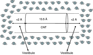
Figure 1: Schematic of the CNT-water system showing the “vestibules” at the openings of the CNT and corresponding dimensions. The CNT is represented as a cylinder surrounded by water molecules.

In this letter, we extend the CMD approach to explore directly the physical parameter space of a complex molecular system. This is accomplished by linking short bursts of MD simulations with continuum algorithms to simultaneously search phase and parameter space. The general formalism is illustrated by studying the parametrically controlled equilibrium between the water-filled and empty state of a short and narrow carbon nanotube (CNT) dissolved in water (Figure 1). The CNT in water serves as a paradigm of a molecular system with nontrivial dynamic and thermodynamic behavior under parametric control. Conventional MD simulations Hummer et al. (2001) showed that for certain interaction strengths between the carbon atoms and water, the molecular system exhibits “bi-phasic” character, with the tube fluctuating on a nanosecond time-scale between a water-filled and an empty state. Such controlled fluctuations in the water occupancy have been suggested as a mechanism to regulate water, proton, and ion transport through biological protein pores Hummer et al. (2001); Beckstein et al. (2001). The computational prediction of filled tubes at strong water-tube interactions has since been confirmed experimentally for somewhat wider tubes Kolesnikov et al. (2004). Important here is that, despite the molecular complexity, the equilibrium thermodynamic calculations required to validate CMD are feasible.

We perform classical MD simulations of a (6,6)-type nanotube of $\sim$13.5 Å length and 8.1 Å diameter in a box of $N_{\mathrm{wat}}=1034$ TIP3P water molecules Jorgensen et al. (1983) under periodic boundary conditions with Ewald electrostatics and a time step of 0.002 ps (additional simulation details as in Refs. Hummer et al. (2001); Sriraman et al. (2005)). We use CMD to explore the thermodynamics and kinetics of tube filling as a function of the “hydrophobicity parameter” $\lambda$ scaling the attractive $r^{-6}$ carbon-water Lennard-Jones interactions: $u_{\mathrm{C-O}}(r)=Ar^{-12}-\lambda Cr^{-6}$ where $A=696,790.7$ kcal mol^-1 Ź² and $C=564.5036$ kcal mol^-1 Å⁶, respectively. In physical experiments, the effect of $\lambda$ on the water-affinity for the CNT pore can be mimicked by changing quantities like water pressure or osmolality. To monitor filling and emptying, we use the water occupancy as a coarse observation variable, $N=\sum_{i=1}^{N_{\mathrm{wat}}}\Theta(r_{i},z_{i})$, where $r_{i}$ and $z_{i}$ are the water radial and axial positions in the cylindrical coordinate system defined by the instantaneous position and orientation of the freely moving CNT (other simulation details as in Hummer et al. (2001)). The weight function is given by $\Theta(r,z)=\exp[-{(r/R_{cyl})}^{6}-{(2z/L_{cyl})}^{6}]$ where $L_{cyl}~{}=~{}17.5$ Å and $R_{cyl}~{}=~{}4.05$ Å are the length and radius, respectively, of a cylindrical region that extends somewhat beyond the $\sim$13.5 Å long CNT to include water molecules near the openings (see Figure 1). By including these “vestibules” of the CNT, we resolve the gradual entry, or exit, of a water molecule without compromising the information about the state of nanotube filling. We found earlier that the tube appears bi-stable for $\lambda\approx 0.8$ Hummer et al. (2001); Waghe et al. (2002); it is predominantly empty below $\lambda\approx 0.7$, and filled above $\lambda\approx 0.9$.

Bi-stability can be succinctly summarized in a bifurcation diagram that reports local maxima of the equilibrium density as a function of $\lambda$ and – in the bi-stable regime – also the intervening saddles. In what follows, we will use short replica MD simulations to construct a kinetically-based coarse bifurcation diagram and compare it to thermodynamics. We will report the fixed points of a timestepper constructed by CMD through the following steps. In the “lifting” step, we create representative initial phase points of the full molecular system. For a given value of the hydrophobicity parameter $\lambda$, we harmonically bias the occupancy $N$ during a short, 15-ps MD run, toward a target $N_{0}$ by adding $U_{bias}=k(N-N_{0})^{2}/2$ to the Hamiltonian ($k=50$ kcal mol^-1 for $N_{0}\geq 1$; $k=80$ kcal mol^-1 for $N_{0}<1$). Five different conformations near each target $N_{0}$ value are saved during the last 5 ps of the constrained run, and 10 sets each of random Maxwell-Boltzmann velocities are assigned to create 50 starting configurations. In the “evolve” step, an unconstrained MD run of $\tau=1$ ps duration is performed for each structure. Finally, in the “restrict” step, the resulting trajectories are projected onto the coarse variable $N$. In particular, the average occupancy $N$ at the end of the short runs defines our CMD timestepper: $\overline{N(\tau;N_{0};\lambda)}\equiv\Phi_{\tau}(N_{0};\lambda)$.

The fixed points for given values of $\lambda$ satisfy

$$f(N;\lambda)\equiv N-\Phi_{\tau}(N;\lambda)=0.$$ (1)

They correspond to metastable empty or full, as well as to unstable, partially filled “transition states”. For small $\tau$ the above equation approximates the differential (steady state) form ${\partial\Phi_{t}(N_{0};\lambda)}/{\partial t}=0$; all our coarse-grained computations can be equivalently performed through this differential form. Fixed points for given $\lambda$ are computed by solving Eq. (1) through a Newton-Raphson type iteration with an appropriate initial guess for $N$:

$$N_{1}=N_{0}-\frac{f(N_{0};\lambda)}{\partial f/\partial N_{0}}$$ (2)

In Eq. (2), $\partial f/\partial N_{0}$ is estimated by computing $N-\Phi_{\tau}(N;\lambda)$ for nearby initial points $N$. Fixed points converged to within ${\cal O}(10^{-3})$. The results (fixed points as a function of $\lambda$) are plotted in Figure 2.

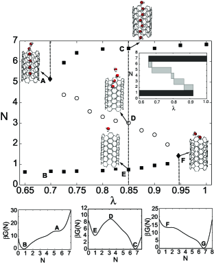
Figure 2: Coarse bifurcation diagram for the CNT-water system. Solid filled squares ($\blacksquare$) correspond to fully filled ($N>5$) and empty states ($N\leq 1)$, respectively. Open circles ($\bigcirc$) correspond to partially filled states, while the filled diamonds ($\blacklozenge$) correspond to the turning points of the coarse bifurcation diagram. Vertical dashed lines indicate the upper (A) and lower (F) turning points, and $\lambda=0.85$ (points C-D-E), respectively. Representative structures for points A-F are indicated by arrows (carbon: gray; oxygen: red; hydrogen: white). The coarse effective free energy surfaces for $\lambda=0.7$, 0.85, and 0.95, respectively, are shown below the main figure. The inset in the top right corner of the main figure shows the effective bifurcation diagram obtained through histogram reweighting.

At the upper (lower) turning points we lose the filled (empty) fixed points. In principle, turning points can be found by computing the entire diagram (using pseudo-arclength continuation Doedel et al. (1991)); however, numerical bifurcation theory provides more efficient algorithms that solve directly for these points (and thus the boundaries of apparent hysteresis in parameter space). In compact notation, $\mathbf{X}=[N,\lambda]^{T}$ is a vector describing the position in the bifurcation diagram; the turning points are roots of the vector-valued function $\mathbf{F}(\mathbf{X})=[N-\Phi_{t}(N;\lambda),1-{\partial{\Phi_{t}(N;\lambda)}}/{\partial N}]^{T}=\mathbf{0}$. To solve these two coupled equations for the critical $N$ and $\lambda$ simultaneously, we use a 2D recursive Newton-Raphson iteration procedure:

$$\mathbf{X}_{1}=\mathbf{X}_{0}-{\Big{[}\frac{\partial\mathbf{F}}{\partial\mathbf{X}}\Big{]}}_{\mathbf{X}_{0}}^{-1}\cdot\mathbf{F}(\mathbf{X}_{0})$$ (3)

The derivatives of the Newton-type iteration,

$$\frac{\partial\mathbf{F}}{\partial\mathbf{X}}=\left[\begin{array}[]{cc}1-\frac{\partial{\Phi_{\tau}(N;\lambda)}}{\partial N}&-\frac{\partial{\Phi_{\tau}(N;\lambda)}}{\partial\lambda}\\ -\frac{\partial^{2}{\Phi_{\tau}(N;\lambda)}}{\partial N^{2}}&-\frac{\partial^{2}{\Phi_{\tau}(N;\lambda)}}{\partial N\partial\lambda}\end{array}\right]~{},$$ (4)

are estimated numerically from replica simulations initiated on a centered “stencil” (i.e., grid) with $|\Delta N|=0.1$ and $|\Delta\lambda|=0.025$ around $\mathbf{X}_{0}=[N_{0},\lambda_{0}]^{T}$. The “lift-evolve-restrict” procedure is implemented and the timesteppers, $\Phi_{\tau}(N;\lambda)$, are computed for each node of the grid. Starting from a good initial guess, the procedure converges after a few ($\sim$5) iteration steps: the updates for $[N,\lambda]^{T}$ and residuals for $\mathbf{F}$ are of order ${\cal O}(10^{-3})$ and ${\cal O}(10^{-2})$, respectively.

Figure 2 shows the resulting coarse bifurcation diagram for the CNT-water system. The two metastable branches of the S-shaped diagram correspond to empty ($N\approx 1$) and filled states ($N\approx 7$). The lower and upper turning points are at $\lambda\approx 0.7$ and 0.95, respectively.

So far, we have taken an entirely dynamic perspective in our computations. To estimate the underlying thermodynamics, knowing that $N$ is a good reaction coordinate Waghe et al. (2002), we assume diffusive dynamics along $N$ in the form of an effective Fokker-Planck (FP) equation:

$$\frac{\partial P(N,t;\lambda)}{\partial t}=\big{[}-\frac{\partial}{\partial N}v(N;\lambda)+\frac{\partial^{2}}{\partial N^{2}}D(N;\lambda)\big{]}P(N,t;\lambda).$$ (5)

The coarse timestepper calculations are precisely what is needed to parametrize this FP:

$$v(N;\lambda)\equiv\frac{\partial\overline{N(t,N_{0};\lambda)}}{\partial t};~{}2D(N;\lambda)\equiv\frac{\partial\sigma^{2}[N(t;N_{0};\lambda)]}{\partial t}$$ (6)

For short simulation times $\tau$, the coarse timestepper (the average of the results of the replica simulations) is used to estimate the drift $v(N;\lambda)$; from the time-dependence of the variance $\sigma^{2}[N(t;N_{0};\lambda)]$ of $N$, we estimate the diffusion coefficient $D(N;\lambda)$. In this notation, the effective free energy $G(N;\lambda)$ for the problem is

$$\beta G(N;\lambda)=-\int_{0}^{N}\frac{v(N^{\prime};\lambda)}{D(N^{\prime};\lambda)}dN^{\prime}+\ln~{}D(N;\lambda)+\mathrm{const.}$$ (7)

Maxima of the equilibrium density $\exp(-\beta G(N;\lambda))$ can be found as zeroes of $v(N;\lambda)-D^{\prime}(N;\lambda)$ [or, ignoring a weak $N$ dependence of $D$, by the zeroes of $v(N;\lambda)$]. Clearly, the fixed points of our coarse timestepper are approximations of the free energy extrema, where metastable and unstable fixed points correspond to well bottoms and intervening saddles, respectively.

In the inset of Figure 2, we show for comparison the thermodynamic bifurcation diagram, indicating the minima and saddles of the equilibrium free energy surfaces $G(N;\lambda)$. This diagram is estimated from three long (132 ns total) equilibrium MD simulations, one in the predominantly filled regime ($\lambda=1$), one in the predominantly empty regime ($\lambda\approx 0.75$), and one in between ($\lambda=0.785$). By combining the 3-dimensional histograms of occupancy fluctuations and water-CNT interaction energies using a weighted histogram method Sriraman et al. (2005); Ferrenberg and Swendsen (1989), we obtain the free energy surface $G(N;\lambda)$ at different $\lambda$ values. To avoid difficulties with insufficient sampling of the observation variable in the equilibrium runs, we coarse-grained $N$ to the nearest integer numbers.

Overall, we find excellent agreement between the coarse bifurcation diagram from multiple short (1-ps) CMD runs, and that from long equilibrium runs. In particular, the location of the metastable and unstable branches is nicely reproduced by the equilibrium results. The main difference is that the lower turning point is at a somewhat lower interaction strength $\lambda\approx 0.66$ compared to 0.7. Such small differences can be due to several factors: (1) The equilibrium-predicted lower turning point lies outside the $\lambda$-range probed by MD and had to be extrapolated. (2) The equilibrium computations were coarse-grained to integer $N$ values. (3) The $N$-dependence of the effective diffusion coefficient was neglected in constructing the kinetic bifurcation diagram; and finally (4) CMD simulations at stationarity probe the dynamic stability of an apparent fixed point over a given time horizon $\tau$. The location of fixed as well as turning points from CMD will depend somewhat on $\tau$. Here, the short runs are about 1 ps long, one order of magnitude shorter than the duration of a typical water uptake or release event $N\rightleftharpoons N+1$ Waghe et al. (2002), assuming Markov-chain dynamics. For parameter values close to the turning points, as the free energy wells become more shallow, typical transition times $N\rightleftharpoons N+1$ become comparable to any fixed $\tau$. As a result, one would expect the CMD turning points to move “inwards,” and the apparent hysteresis range to shrink Haataja et al. (2004).

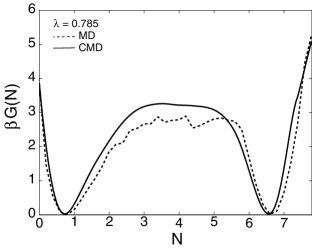
Figure 3: Coarse free energy surface as a function of N for $\lambda=0.785$ where the empty and filled wells have equal depth. Results from equilibrium MD (dashed) and CMD [from Eq. (7); solid] are shown. The effective free energy predicted by CMD agrees well with that of 19-ns long equilibrium MD simulations.

Our CMD calculations have so far been local in $N$-$\lambda$ space. As an example of a parametric search involving global properties, we next locate the critical hydrophobicity parameter value at which the filled and empty states have (approximately) equal populations. We formulate this as a fixed point problem that we solve iteratively. Given an initial guess of $\lambda$ we first solve for the two metastable fixed points [$N_{\mathrm{empty}}(\lambda)$ and $N_{\mathrm{full}}(\lambda)$]. We then consider any reasonable path between the two (parametrized by the coarse observable $N$), discretize it, and estimate (through locally initialized and executed MD experiments and quadrature) the state dependent drift and diffusion coefficient in the FP equation, Eq. (5). Finally, using Eq. (7), we compute $G(N;\lambda)$. To solve the equation $\Delta G(\lambda)\equiv G(N_{\mathrm{full}};\lambda)-G(N_{\mathrm{empty}};\lambda)=0$ for the critical $\lambda$ we use a contraction mapping with numerically estimated derivatives. $G(N;\lambda)$ was computed as follows: From different initial configurations for $0\leq N_{i}\leq 8$, we run 50 short ($\tau$ = 1 ps) replica simulations. By robust linear fits to the evolution of $\overline{N(t;N_{i};\lambda)}$ and $\sigma^{2}[N(t;N_{i};\lambda)]$, we estimate $v(N)$ and $D(N)$ and compute $\beta G(N)$ from Eq. (7) by integration through a smooth spline approximation to the data. As illustrated in Figure 3, the critical $\lambda$ value is approximately 0.785, and this is confirmed by equilibrium MD simulations. In particular, the MD and CMD free energy surfaces at this critical parameter value are in excellent agreement. We note that for equal populations in the two wells, the free-energy gradients estimated by CMD are relatively small, resulting in particularly reliable free energy surfaces, with larger deviations expected in regimes where one or the other well dominates. Finally, we note that CMD in combination with Kramers theory for diffusive barrier crossing, produces accurate estimates of the rate coefficients for escape from the metastable filled and empty states, when compared with equilibrium MD [$\sim$1/(140 ps) vs. $\sim$1/(190 ps) from MD at the transition midpoint, $\lambda=0.785$].

We illustrated the extension of the CMD approach to the exploration of parameter space of molecular systems. Our computational methods are general and can be used to study metastability boundaries in other systems (e.g., kinetic Monte Carlo Haataja et al. (2004); Makeev or Brownian Dynamics Graham ). Linking continuum nonlinear dynamics computation (fixed point, continuation, integration or bifurcation algorithms) with MD simulations has the potential to accelerate parametric exploration of dynamic as well as thermodynamic features. The knowledge of good reaction coordinates is crucial for the success of this approach; determining such coordinates based on data is the subject of intense current research Bolhuis et al. (2002); Hummer (2004); Nadler et al. (2004).

Acknowledgments Support in part by the Intramural Research Program of the NIH, NIDDK (GH) and NSF/ITR and DARPA/ARO (SS, IGK) is gratefully acknowledged.

References

- Voter (1997) A. F. Voter, Phys. Rev. Lett. 78, 3908 (1997).
- Bolhuis et al. (2002) P. G. Bolhuis, D. Chandler, C. Dellago, and P. L. Geissler, Annu. Rev. Phys. Chem. 53, 291 (2002).
- Schütte et al. (1999) C. Schütte, A. Fischer, W. Huisinga, and P. Deuflhard, J. Comp. Phys. 151, 146 (1999).
- Laio and Parrinello (2002) A. Laio and M. Parrinello, Proc. Natl. Acad. Sci. U.S.A. 99, 12562 (2002).
- Hummer and Kevrekidis (2003) G. Hummer and I. G. Kevrekidis, J. Chem. Phys. 118, 10762 (2003).
- Kevrekidis et al. (2004) I. G. Kevrekidis, C. W. Gear, and G. Hummer, AIChE J. 50, 1346 (2004).
- Zwanzig (2001) R. Zwanzig, Nonequilibrium Statistical Mechanics (Oxford University Press, New York, 2001).
- Hummer et al. (2001) G. Hummer, J. C. Rasaiah, and J. P. Noworyta, Nature 414, 188 (2001).
- Beckstein et al. (2001) O. Beckstein, P. C. Biggin, and M. S. P. Sansom, J. Phys. Chem. B 105, 12902 (2001).
- Kolesnikov et al. (2004) A. I. Kolesnikov, J. M. Zanotti, C. K. Loong, P. Thiyagarajan, A. P. Moravsky, R. O. Loutfy, and C. J. Burnham, Phys. Rev. Lett. 93, 035503 (2004).
- Jorgensen et al. (1983) W. L. Jorgensen, J. Chandrasekhar, J. D. Madura, R. W. Impey, and M. L. Klein, J. Chem. Phys. 79, 926 (1983).
- Sriraman et al. (2005) S. Sriraman, I. G. Kevrekidis, and G. Hummer, J. Phys. Chem. B 109, 6479 (2005).
- Waghe et al. (2002) A. Waghe, J. C. Rasaiah, and G. Hummer, J. Chem. Phys. 117, 10789 (2002).
- Doedel et al. (1991) E. J. Doedel, H. B. Keller, and J. P. Kernevez, Int. J. Bif. Chaos. 1, 493 (1991).
- Ferrenberg and Swendsen (1989) A. M. Ferrenberg and R. H. Swendsen, Phys. Rev. Lett. 63, 1195 (1989).
- Haataja et al. (2004) M. Haataja, D. J. Srolovitz, and I. G. Kevrekidis, Phys. Rev. Lett. 92, 160603 (2004).
- (17) A. G. Makeev, D. Maroudas, A. Z. Panagiotopoulos and I. G. Kevrekidis, J. Chem. Phys. 117, 8229 (2002).
- (18) C. Siettos, M. D. Graham and I. G. Kevrekidis, J. Chem. Phys. 118 10149 (2003).
- Hummer (2004) G. Hummer, J. Chem. Phys. 120, 516 (2004).
- Nadler et al. (2004) B. Nadler, S. Lafon, R. C. Coifman, and I. G. Kevrekidis, Appl. Comp. Harm. Anal. (2004), in press.