Evidence for s-wave pairing from measurement on lower critical field in $MgCNi_{3}$

Abstract

Magnetization measurements in the low field region have been carefully performed on a well-shaped cylindrical and an ellipsoidal sample of superconductor $MgCNi_{3}$. Data from both samples show almost the same results. The lower critical field $H_{c1}$ and the London penetration depth $\lambda$ are thus derived. It is found that the result of normalized superfluid density $\lambda^{2}(0)/\lambda^{2}(T)$ of $MgCNi_{3}$ can be well described by BCS prediction with the expectation for an isotropic s-wave superconductivity.

I INTRODUCTION

The pairing symmetry is very essential for uncovering the mechanism both for conventional and high-$T_{c}$ superconductivity. The recently discovered intermetallic perovskite $MgCNi_{3}$ superconductorhe-nature is regarded as a bridge between conventional superconductors and high-$T_{c}$ cuprates, and the issue concerning its symmetry of order parameter has attracted considerable attention. However, pairing symmetry about $MgCNi_{3}$ remains highly controversial in reported literatures. NMRsinger-NMR , specific heatlin-SH , scanning tunneling measurementkinoda-scanning and point contact tunneling spectrashan-tunneling favor the s-wave pairing in $MgCNi_{3}$. On the other hand, the earlier theoretical calculationrosner-prl , the tunneling spectramao-tunneling and the penetration depth measurementprozorov-penetration support non-s-wave superconductivity. Recently a two-band s-wave model has been proposed by W$\ddot{a}$lte et al.walte who try to explain the complex behavior observed in $MgCNi_{3}$.

In this paper, we derive the thermodynamic parameters $H_{c1}$ and $\lambda$ of two $MgCNi_{3}$ samples by careful magnetization measurement. It is found that the normalized superfluid density, $\lambda^{2}(0)/\lambda^{2}(T)$, can be described by BCS prediction for a s-wave pairing symmetry. Therefore, our magnetization data support the conventional single band s-wave superconductivity in $MgCNi_{3}$.

This paper is organized as follows: The samples and experimental details are presented in section II. The data and discussions are given in section III. And section IV gives the summary.

II SAMPLES AND EXPERIMENTAL DETAILS

The polycrystalline $MgCNi_{3}$ sample investigated here has been prepared by powder metallurgy method, and the details of preparation can be found elsewhereren-sample . The superconducting transition temperature is 6.9 K measured by both magnetization [ ac susceptibility ( $f=333$ Hz, $H_{ac}=1$ Oe ) and dc diamagnetization shown in Fig. 1(a) ] and resistivity measurement. The $M(T)$ curves show a sharp transition with the transition width less than 0.5 K. The x-ray diffraction ( XRD ) analysis presented in Fig. 1 (b) shows that all diffraction peaks are from the $MgCNi_{3}$ phase, which indicates that the sample is nearly of single phase.

Figure 1: (a) The ac susceptibility curves of $MgCNi_{3}$ measured by MagLab with ac field 1 Oe and frequency 333 Hz. The inset gives the ZFC and FC dc diamagnetization at 20 Oe measured by SQUID. (b) XRD patterns of the $MgCNi_{3}$.

In order to minimize the demagnetization factor, one sample ( denoted as $S$-$c$ ) has been carefully cut and ground to a cylinder with a diameter of 1.1 mm and length of 7.0 mm. The demagnetization factor in this situation is almost negligible since the field has been applied along the axis of the cylinder. Another sample ( denoted as $S$-$e$ ) has been polished to an ellipsoid with semi-major axis a=3.74 mm and semi-minor axis b=1.5 mm. The demagnetization factor for the ellipsoidal sample is $n=(1-\frac{1}{e^{2}})(1-\frac{1}{2e}\cdot\ln\frac{1+e}{1-e})\approx 0.136$, with $e=\sqrt{1-b^{2}/a^{2}}$. The magnetic fields have been applied parallel to the longitudinal axis of the samples.

The magnetic measurements are mainly carried out on an Oxford cryogenic MagLab system ( MagLab12Exa, with temperature down to 1.5 $K$ ) and checked by a quantum design superconducting interference device ( SQUID, MPMS 5.5 T ). After zero-field cooled ( ZFC ) from 25 K to a desired temperature, the magnetization curve $M(H)$ is measured with the applied magnetic field swept slowly up to 1000 Oe ( $\gg$ $H_{c1}$ ). It is important to note that the magnet has been degaussed at T= 25 K in order to eliminate the remanent field before each measurement. It is essential to do degaussing since otherwise even 5 Oe residual field may cause significant effect on the result of magnetization.

III EXPERIMENTAL DATA AND DISCUSSIONS

In this section, the processes to obtain the superconducting parameters by magnetization measurement have been reported in detail for two $MgCNi_{3}$ samples, one is a cylinder and another is an ellipsoid.

III.1 The cylindrical sample ( $S$-$c$ )

The curves of dc magnetization are shown in Fig. 2. The temperature varies between 1.57 K and 6.88 K with steps 0.2 K ( some 0.4 K ). All curves show clearly the common linear dependence of the magnetization on field caused by Meissner effect at low fields, and this extrapolated common line is the so-called “Meissner line”( ML ). The optimal ML ( solid line in Fig.2 ) is achieved by doing linear fit $M(H)$ of the lowest temperature ( 1.57 K ) at low fields, which represents the magnetization curve of Meissner state. The value of H_c1 is determined by examining the point of departure from linearity on the initial slope of the magnetization curve ( ML ) with a certain criterion. The results of subtracting this ML from magnetization curves are plotted in Fig. 3 and the $\Delta M$ between $7.0\times 10^{-4}$ and $1.4\times 10^{-3}$ emu are shown in the inset with an enlarged view. All curves show a fast drop to the resolution of device when the real $H_{c1}$ is approached, so the value of H_c1 is easily obtained by choosing a proper criterion of $\Delta$M. The H${}_{c1}(T)$ acquired by using criteria of $\Delta M=7.0\times 10^{-4}$ and $1.1\times 10^{-3}$ emu are shown in Fig. 4. Then the penetration depth $\lambda(T)$ can be achieved from H${}_{c1}(T)$ by

$$H_{c1}=\frac{\rm\Phi_{0}}{\rm 4\pi\lambda^{2}}\ln\kappa$$ (1)

and they are displayed in the inset of Fig. 4. Here $\Phi_{0}=hc/2e\approx 2\times 10^{-7}G\cdot cm^{2}$ is the flux quantum, and $\kappa$ is the Ginzburg-Landau parameter. We take $\kappa$ as constant since it is a weakly temperature dependent parameter.

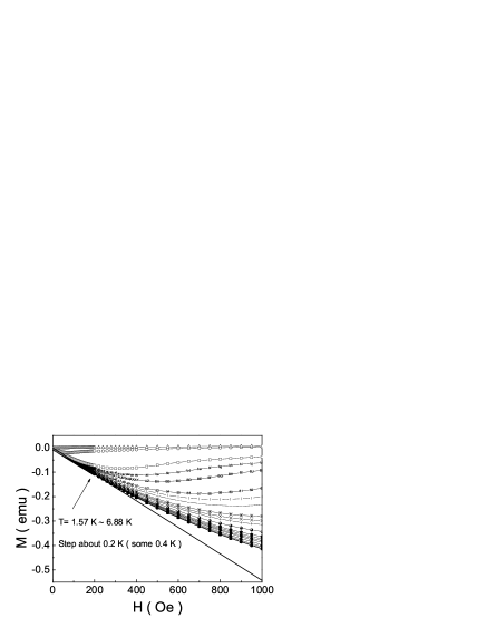
Figure 2: The magnetization curves of $M(H)$ for $MgCNi_{3}$. The solid line is the “Meissner line” defined in the text. The temperature is varied from 1.57 K to 6.88 K from bottom to top, with step about 0.2 K ( some 0.4 K ). It is found that the initial slope of all the curves is the same.

Figure 3: The difference between the “Meissner line” and the $M(H)$ curves. $\Delta M$ is shown in logarithmic scale. The inset shows the enlarged $\Delta M$ ( between $7.0\times 10^{-4}$ and $1.4\times 10^{-3}$ emu ).

Figure 4: The temperature dependence of the nominal $H_{c1}$ and $\lambda$ ( inset ). $H_{c1}(T)$ is obtained by using criterion of $\Delta M=7.0\times 10^{-4}$ ( open circles ) and $1.1\times 10^{-3}$ emu ( solid circles ), respectively. Error bars are given for determining the nominal $H_{c1}$ and $\lambda$. Lines are guides to the eyes.

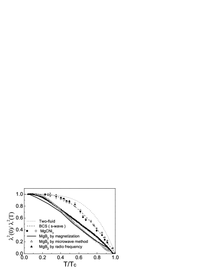
Figure 5: The temperature dependence of $\lambda^{2}(0)/\lambda^{2}(T)$ for $MgCNi_{3}$ and $MgB_{2}$. The values of $\lambda^{2}(0)/\lambda^{2}(T)$ are obtained by $H_{c1}(T)$ using criteria of $\Delta M$ equal $7.0\times 10^{-4}$ ( open circles ) and $1.1\times 10^{-3}$ emu ( solid circles ) for $MgCNi_{3}$ and $1.0\times 10^{-4}$ emu for $MgB_{2}$( solid). The prediction by two-fluid model ( dotted ) and BCS s-wave( dashed ) are also shown. The data of open and solid triangles are the experimental measurement by microwave resonator method and radio frequency technique for $MgB_{2}$, respectively ( from Ref.[klein-appliedSC, ] and Ref.[manzano-prl, ] ).

The values of nominal H_c1 and $\lambda$ seem to be criterion dependent in this method, however temperature dependence of $H_{c1}$ and $\lambda(T)$ are found to be weekly criterion dependent if the data is normalized by the zero temperature values ( see $\lambda^{2}(0)/\lambda^{2}(T)$ in Fig.5 ) . In addition, $\Delta M$ drops sharply with decreasing magnetic field, the use of lower $\Delta M$ value in our criterion will not result in a much different $H_{c1}(T)$ curve. If not specially mentioned, the discussion is based on the data using the criterion of $7.0\times 10^{-4}$ emu hereinafter. At the temperatures below 2.8 K ( $<$ 0.4 $T_{c}$ ), the values of $H_{c1}(T)$ and $\lambda(T)$ are almost constant despite the lack of the data below 1.5 K. This may imply the conventional s-wave nature in $MgCNi_{3}$, because the finite energy gap manifests itself with an exponentially activated temperature dependence of thermodynamic parameters. This can be further confirmed in the following discussion on superfluid density. Worthy of noting is that, it is very difficult to distinguish a slight difference of $H_{c1}$ ( or 1/$\lambda^{2}$ ) in low temperature region between different pairing symmetries, for example for an ideal s-wave, an exponential dependence is anticipated, for a dirty d-wave, a quadratic form $\rho_{s}(T)=\rho_{s}(0)-\alpha T^{2}$ is expected. Here we use an alternative way, i.e, to fit the data in intermediate and high temperature region to extract useful message for pairing symmetry.

As we know, the total superfluid density $\rho_{s}$ is proportional to $\lambda^{-2}(T)$, and $\lambda^{2}(0)/\lambda^{2}(T)$ represents the normalized superfluid density. In Fig. 5, we display the temperature dependence of $\lambda^{2}(0)/\lambda^{2}(T)$ of $MgCNi_{3}$ with $\lambda(0)$ as a fit parameter. The predictions of BCS s-wave( dashed ) and two-fluid model ( dotted ) are also shown. According to the BCS theory for clean superconductorsTinkham ; kim-prb , the normalized superfluid density $\lambda^{2}(0)/\lambda^{2}(T)$ is expressed as follows:

$$\frac{\lambda^{2}(0)}{\lambda^{2}(T)}=1-2\int^{\infty}_{\Delta(T)}{(-\frac{\partial{f(E)}}{\partial{E}})D(E)}\mathrm{d}E$$ (2)

where $\Delta(T)$ is the BCS superconducting energy gap, $f(E)=1/[exp(-E/{k_{B}}T)+1]$ is the Fermi distribution function, and $D(E)=E/{(E^{2}-\Delta^{2}(T))^{1/2}}$ is the quasiparticle density of states. The most appropriate superconducting gap $\Delta(0)=1.86k_{b}T_{c}$ is chosen in our BCS calculation with $T_{c}=6.9K$, and this value is reasonable for $MgCNi_{3}$ because the generally reported results are larger than the conventional BCS value($1.76k_{b}T_{c}$). It is found that $\lambda^{2}(0)/\lambda^{2}(T)$ of $MgCNi_{3}$ can be well described by the s-wave BCS theory with a single gap, but the two-fluid model shows a substantial deviation. This suggests the s-wave nature of superconductivity in $MgCNi_{3}$, which is consistent with our previous conclusion reached by point-contact-tunnelingshan-tunneling . Later on we will show that our results are not compatible with any other pairing symmetry with nodes on the gap function which normally contributes a power law dependence to the temperature dependence $\rho_{s}$.

For the sake of comparison, the temperature dependence of the normalized superfluid density in $MgB_{2}$ obtained by exactly the same magnetization methodli-MgB2 is also shown in Fig. 5, with $\lambda(0)$ as a fit parameter. Clearly the data can not be understood in isotropic s-wave BCS theory or two-fluid model because of the two-gap characteristic of $MgB_{2}$choi-natue ; kang-cond . The data obtained from this simple magnetization method on $MgB_{2}$ was found to be close to that determined by more elegant microwave methodklein-appliedSC and radio frequency techniquemanzano-prl , which can be seen from Fig. 5. This indicates that the same magnetization method used in $MgCNi_{3}$ to get $H_{c1}$ and $\lambda$ is reliable, and the corresponding results are plausible.

One may argue whether the $H_{c1}$ obtained here is the lower critical field of grains because of the polycrystalline nature of our sample. In our magnetization experiment, the nominal $H_{c1}(0)$ of our sample is about 145.1 Oe. Combined with $H_{c2}(0)$ ( $1.18\times 10^{5}$ Oe ) determined from our previous measurement of specific-heatshan-carbon , we can reach that the value of $\kappa$ is 39 and $H_{c}(0)$ equals to 2165 Oe by Eqs. (3, 4). The value of coherence length is 5.3 nm obtained by Eq. (5).

$$H_{c1}(T)=\frac{1}{\sqrt{2}}H_{c}(T)\frac{1}{\kappa}\ln\kappa$$ (3)

$$H_{c2}(T)={\sqrt{2}}H_{c}(T)\kappa$$ (4)

$$\xi(0)={\sqrt{\Phi_{0}/2\pi{H_{c2}(0)}}}$$ (5)

And the value of $\lambda(0)$ is about 200.1 nm. All these values of parameters are in the range of the reported results of $MgCNi_{3}$ by other techniques( see collected parameters in Ref.[walte, ] ). This manifests that $H_{c1}$ measured here reflects the bulk property. In addition, the value of $\xi$ for $MgCNi_{3}$ is quite large, so that the influence of the grain boundary is weak.

Another argument is that the nominal $H_{c1}$ relation obtained in our experiment may not reflect the true $H_{c1}$ but the flux entry field because of the Bean-Livingston surface barrier and effects of sample corners geometrical barriers. However, we would argue that the influence of surface barrier is not important to our cylindrical sample, since the magnetization hysteresis loops are very symmetric in the temperature and filed regimes we measured. In order to further verify the validity of this method to obtain $H_{c1}$, we have repeated the same measurement for an ellipsoidal sample. The data and the discussion are presented below.

III.2 The ellipsoidal sample ( $S$-$e$ )

The curves of dc magnetization are shown in Fig. 6 and the temperature varies between 1.59 K and 6.90 K with steps about 0.1 K . The optimal “Meissner line”( solid line in Fig.6 ) has been determined in the same way as for the cylindrical sample. Subtracting this ML from the magnetization data yields the $\Delta M$ curves plotted in Fig. 7. The H${}_{c1}(T)$ acquired by using criteria of $\Delta M=3.2\times 10^{-4}$ and $1.0\times 10^{-3}$ emu are shown in Fig. 8, and the demagnetization factor n ( $\approx 0.136$ ) has been taken into account. Then the penetration depth $\lambda(T)$ can be achieved from Eq(1) and they are displayed in the inset of Fig. 8. The normalized temperature dependence of $\lambda^{2}(0)/\lambda^{2}(T)$ of $MgCNi_{3}$ is shown in Fig. 9. One can clearly see that the data from the ellipsoidal sample is almost identical to that for the cylindrical sample, showing a trivial influence of either the geometrical or surface barrier in our present samples.

Figure 6: The magnetization curves of $M(H)$ for the ellipsoidal $MgCNi_{3}$ sample. The solid line is the “Meissner line”. The temperature is varied from 1.59 K to 6.90 K ( from bottom to top ), with step about 0.1 K .

Figure 7: The difference between the “Meissner line” and the $M(H)$ curves. $\Delta M$ is shown in logarithmic scale.

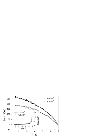
Figure 8: The temperature dependence of the nominal $H_{c1}$ and $\lambda$ (inset). Lines are guides to the eyes.

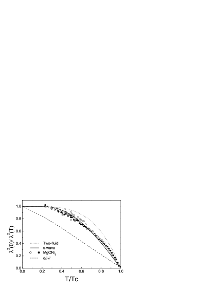
Figure 9: The temperature dependence of $\lambda^{2}(0)/\lambda^{2}(T)$ for ellipsoidal $MgCNi_{3}$ sample. The values of $\lambda^{2}(0)/\lambda^{2}(T)$ are obtained by $H_{c1}(T)$ using criteria of $\Delta M$ equal $3.2\times 10^{-4}$ ( open circles ) and $1.0\times 10^{-3}$ emu ( solid circles ). The prediction by two-fluid model ( dotted ), BCS s-wave ( solid ) and pure d-wave ( dashed ) are also shown.

In addition, we have calculated the superfluid density assuming a nodal gap with d-wave symmetry. Under the frame of the BCS theory, if the gap has a d-wave-like node, the normalized superfluid density $\lambda^{2}(0)/\lambda^{2}(T)$ is written as

$$\frac{\lambda^{2}(0)}{\lambda^{2}(T)}=1-\frac{1}{\pi}\int^{2\pi}_{0}\int^{\infty}_{\Delta(T,\theta)}{-\frac{\partial{f(E)}}{\partial{E}}D(E)}\mathrm{d}E\mathrm{d}\theta$$ (6)

with $f(E)=1/[exp(-E/{k_{B}}T)+1]$, $\Delta(T,\theta)=\Delta_{0}(T)\cdot\cos 2\theta$ and $D(E)=E/{(E^{2}-\Delta^{2}(T,\theta))^{1/2}}$. The calculated d-wave results are shown in Fig. 9 with dashed line. For $\mathrm{p}_{x}$-wave symmetry with $\Delta(T,\theta)=\Delta_{0}(T)\cdot\sin\theta$, we found that the calculated temperature dependence of $\lambda^{2}(0)/\lambda^{2}(T)$ is close to that of d-wave, and far from our experiment data. The predictions of s-wave BCS ( solid ) and two-fluid model ( dotted ) are also shown in Fig. 9. It is found that our data can only be well described by the s-wave model. Together with the results for the cylindrical sample, we conclude that $MgCNi_{3}$ is most likely an isotropic s-wave superconductor.

IV SUMMARY

To summarize, we have measured the M-H curves of two $MgCNi_{3}$ samples with cylindrical and ellipsoidal shapes and obtained their lower critical field $H_{c1}(T)$ and $\lambda(T)$. The temperature dependence of normalized superfluid density is consistent with the s-wave BCS theory. All these indicate that $MgCNi_{3}$ may possess an isotropic s-wave gap, which is in sharp contrast to $MgB_{2}$.

Note added: The recent report of carbon isotope effect in MgCNi₃ by T. Klimczuk and R.J. Cava indicates that carbon-based phonons play an essential role in the superconducting mechanism Cava-prb .

- (1) T. He, Q. Huang, A. P. Ramirez, Y. Wang, K. A. Regan, N. Rogado, M. A. Hayward, M. K. Haas, J. S. Slusky, K. Inumara, H. W. Zandbergen, N. P. Ong, and R. J. Cava, Nature (London) 411, 54 (2001).
- (2) P. M. Singer, T. Imai, T. He, M. A. Hayward, and R. J. Cava, Phy. Rev. Lett. 87, 257601 (2001).
- (3) J. Y. Lin, P. L. Ho, H. L. Huang, P. H. Lin, Y. L. Zhang, R. C. Yu, C. Q. Jin, and H. D. Yang, Phys. Rev. B 67, 052501 (2003).
- (4) G. Kinoda, M. Nishiyama, Y. Zhao, M. Murakami, N. Koshizuka, and T. Hasegawa, Jpn. J. Appl. Phys. 40, L1365 (2001).
- (5) L. Shan, H. J. Tao, H. Gao, Z. Z. Li, Z. A. Ren, G. C. Che, and H. H. Wen, Phys. Rev. B 68, 144510 (2003).
- (6) H. Rosner, R. Weht, M. D. Johannes, W. E. Pickett, and E. Tosatti, Phys. Rev. Lett. 88, 027001 (2002).
- (7) Z. Q. Mao, M. M. Rosario, K. D. Nelson, K. Wu, I. G. Deac, P. Schiffer, Y. Liu, T. He, K. A. Regan, and R. J. Cava, Phys. Rev. B 67, 094052 (2003).
- (8) R. Prozorov, A. Snezhko, T. He, and R. J. Cava, Phys. Rev. B 68, 180502(2003).
- (9) A. Wlte, G. Fuchs, K. H. Mller, A. Handstein, K. Nenkov, V. N. Narozhnyi, S. L. Drechsler, S. Shulga, and L. Schultz, cond-mat/0402421 (2004).
- (10) Z. A. Ren, G. C. Che, S. L. Jia, H. Chen, Y. M. Ni, G. D. Liu, and Z. X. Zhao, Physica C 371, 1 (2002).
- (11) M. Tinkham, Introduction to Superconductivity, 2nd ed. ( McGraw-Hill, New York 1996), p93.
- (12) M. S. Kim, J. A. Skinta, T. R. Lemberger, W. N. Kang, H. J. Kim, E.M Choi, and S. I. Lee, Phys. Rev. B 66, 064511 (2002).
- (13) S. L. Li, H. H. Wen, Z. W. Zhao, Y. M. Ni, Z. A. Ren, G. C. Che, H. P. Yang, Z. Y. Liu, and Z. X. Zhao, Phys. Rev. B 64, 094522 (2001).
- (14) H. J. Choi, D. Roundy, H. Sun, M. L. Cohen, and S. G. Louie, Nature 418, 758 (2001).
- (15) B. Kang, H. J. Kim, M. S. Park, K. H. Kim, and S. I. Lee, cond-mat/0403140.
- (16) N. Klein, B. B. Jin, R. Wrdenweber, P. Lahl, W. N. Kang, Hyeong-Jin Kim, Eun-Mi Choi, Sung-IK Lee, T. Dahm, and K. Maki, IEEE Trans. On Appl.Supercond. 13, 3253 (2003).
- (17) F. Manzano, A. Carrington, N. E. Hussey, S. Lee, A. Yamamoto, and S. Tajima, Phys. Rev. Lett. 88, 047002 (2002).
- (18) L. Shan, K. Xia, Z. Y. Liu, H. H. Wen, Z. A. Ren, G. C. Che, and Z. X. Zhao, Phys. Rev. B 68, 024523 (2003).
- (19) T. Klimczuk and R.J. Cava, cond-mat/0410504.