Intermittency in Two-Dimensional Turbulence with Drag

Abstract

We consider the enstrophy cascade in forced two-dimensional turbulence with a linear drag force. In the presence of linear drag, the energy wavenumber spectrum drops with a power law faster than in the case without drag, and the vorticity field becomes intermittent, as shown by the anomalous scaling of the vorticity structure functions. Using previous theory, we compare numerical simulation results with predictions for the power law exponent of the energy wavenumber spectrum and the scaling exponents of the vorticity structure functions $\zeta_{2q}$. We also study, both by numerical experiment and theoretical analysis, the multifractal structure of the viscous enstrophy dissipation in terms of its Rényi dimension spectrum $D_{q}$ and singularity spectrum $f(\alpha)$. We derive a relation between $D_{q}$ and $\zeta_{2q}$, and discuss its relevance to a version of the refined similarity hypothesis. In addition, we obtain and compare theoretically and numerically derived results for the dependence on separation $r$ of the probability distribution of $\delta_{\vec{r}}\omega$, the difference between the vorticity at two points separated by a distance $r$. Our numerical simulations are done on a $4096\times 4096$ grid.

I Introduction

Two-dimensional Navier-Stokes turbulence has attracted much interest because of its relevance to a variety of natural flow phenomena. Examples are plasma in the equatorial ionosphere Kelley and Ott (1978) and the large-scale dynamics of the Earth’s atmosphere and oceans Nastrom and Gage (1985). In the laboratory, experiments that are close to two-dimensional, such as soap film flow Kellay et al. (1998); Rutgers (1998) and magnetically forced stratified flow Paret et al. (1999), have been conducted. In addition, rotating fluid systems Baroud et al. (2002) are used to study quasi-two-dimensional turbulence and its relevance to large-scale planetary flow. Ref. Kellay and Goldburg (2002) gives a review of some recent experiments in two-dimensional turbulence.

In many of the situations involving two-dimensional turbulence, there are regimes where drag is an important physical effect. In the ionospheric case, there is drag friction of the plasma as it moves relative to the neutral gas background (due to ion-neutral collision). For geophysical flows and rotating fluid experiments, viscosity and the no-slip boundary condition give rise to Ekman friction. In this case the three-dimensional flow is often modeled as two-dimensional outside the layer adjoining the no-slip boundary, and the effect of the boundary layer manifests itself as drag in the two-dimensional description. For soap film and magnetically forced flows, friction is exerted on the fluids by surrounding gas and the bottom of the container, respectively. In all these cases, the drag force can be modeled as proportional to the two-dimensional fluid velocity $\vec{v}$, thus the describing Navier-Stokes momentum equation becomes,

$$\frac{\partial\vec{v}}{\partial t}+(\vec{v}\cdot\nabla)\vec{v}=-\frac{1}{\rho}\nabla p+\nu\nabla^{2}\vec{v}-\mu\vec{v}+\vec{f}\ ,$$ (1)

where $\rho$ is the fluid density, $\mu$ is the drag coefficient, $\nu$ is the kinematic viscosity and $\vec{f}$ is an external forcing term. In two-dimensions, the system can be described by the scalar vorticity field $\omega$ whose equation of motion is obtained by taking the curl of Eq. (1),

$$\frac{\partial\omega}{\partial t}+\vec{v}\cdot\nabla\omega=\nu\nabla^{2}\omega-\mu\omega+f_{\omega}$$ (2)

with $\omega=\hat{z}\cdot\nabla\times\vec{v}$ and $f_{\omega}=\hat{z}\cdot\nabla\times\vec{f}$, $\hat{z}$ being the unit vector perpendicular to the plane. In our studies, the forcing will be taken to be localized at small wavenumbers ($k$) with a characteristic wavenumber $k_{f}$, and incompressibility, $\nabla\cdot\vec{v}=0$, will be assumed.

According to Kraichnan, for two-dimensional turbulence with no drag and very small viscosity, for $k\gg k_{f}$, up to the viscous cutoff $k_{d}$, enstrophy cascades from small to large $k$ Kraichnan (1967). As a result, the energy wavenumber spectrum $E(k)$ has a power law behavior with logarithmic correction Kraichnan (1971), $E(k)\sim k^{-3}[\ln(k/k_{f})]^{-1/3}$ for $k_{f}\ll k\ll k_{d}$. In the presence of a linear drag, the energy spectrum drops with a power law faster than the case with no drag Nam et al. (2000a, b); Bernard (2000),

$$E(k)\sim k^{-(3+\xi)}\qquad(\xi>0)\ ,$$ (3)

and there is no logarithmic correction. A result similar to Eq. (3) has been obtained for the closely related problem of chaotically advected finite lifetime passive scalars Chertkov (1998); Abraham (1998); Nam et al. (1999). (See Section II.1 for a discussion of the relationship between vorticity in two-dimensional turbulence with drag and finite lifetime passive scalars in Lagrangian chaotic flows.)

Furthermore, the vorticity field is intermittent as indicated by (i) anomalous scaling of the vorticity structure function, (ii) scale dependence of the vorticity difference distribution function, and (iii) multifractal properties of the enstrophy dissipation field. Intermittency in the closely related problem of chaotically advected finite lifetime passive scalars was originally studied by Chertkov Chertkov (1998) using a model flow in which the velocity field was spatially linear and $\delta$-correlated in time (white noise). This model successfully captures the generic intermittent aspect of the problem not . With respect to the situation of interest to us in the present paper, it is a priori unclear to what extent the $\delta$-correlated model yields results that approximate quantitative results for intermittency measures obtained from experiments (numerical or real). This will be discussed further in Secs. III.2 and IV.

The structure function of order $2q$, $S_{2q}(\vec{r})$ is defined as the $(2q)^{\mathrm{th}}$ moment of the absolute value of the vorticity difference $\delta_{\vec{r}}\omega=\omega(\vec{x}+\vec{r})-\omega(\vec{x})$. Assuming that the system is homogeneous and isotropic, the structure functions depend on $r=|\vec{r}|$ only. For the case with drag ($\mu>0$), it is found that, in the enstrophy cascade range $(k_{d}^{-1}\ll r\ll k_{f}^{-1})$, $S_{2q}(r)$ scales with $r$ as,

$$S_{2q}(r)=\langle|\delta_{\vec{r}}\omega|^{2q}\rangle\sim r^{\zeta_{2q}}$$ (4)

with $\zeta_{2q}>0$. Furthermore, the vorticity structure functions show anomalous scaling; that is, $\zeta_{2q}$ is a nonlinear function of $q$. The nonlinear dependence of $\zeta_{2q}$ on $q$ indicates that the vorticity field is intermittent. In contrast, in the absence of drag ($\mu=0$), it is predicted that $\omega(\vec{x})$ wiggles rapidly (i.e., on the scale $k_{d}^{-1}$) and homogeneously in space. In terms of Eq. (4), this corresponds to $\zeta_{2q}=0$ for $\mu=0$ Falkovich and Lebedev (1994); Eyink (1996); Paret et al. (1999).

The intermittency of the vorticity field also manifests itself as a change in shape or form of the probability distribution function of the vorticity difference $\delta_{\vec{r}}\omega$ with the separating distance $r$. It can be shown that if the probability distribution function $\bar{P}_{r}(X_{\vec{r}})$ of the standardized vorticity difference,

$$X_{\vec{r}}=\frac{\delta_{\vec{r}}\omega}{\sqrt{\langle(\delta_{\vec{r}}\omega)^{2}\rangle}}\ ,$$ (5)

is independent of $r$, then $\zeta_{2q}$ increases linearly with $q$: From Eq. (4) and Eq. (5),

$$S_{2q}(r)=\langle|\delta_{\vec{r}}\omega|^{2}\rangle^{q}\int|X_{\vec{r}}|^{2q}\bar{P}_{r}(X_{\vec{r}})\,dX_{\vec{r}}\ ,$$ (6)

and, if $\bar{P}_{r}(X_{\vec{r}})$ is independent of $r$, for $r$ in the cascade range, then the only $r$-dependence of $S_{2q}(r)$ comes through the term $\langle|\delta_{\vec{r}}\omega|^{2}\rangle^{q}$, implying $\zeta_{2q}=q\zeta_{2}$; that is, $\zeta_{2q}$ is linearly proportional to $q$. Such collapse of $\bar{P}_{r}(X_{\vec{r}})$ for different values of $r$ has been observed in an experiment Paret et al. (1999) where drag is believed to be unimportant. When the effect of drag is not negligible, $\bar{P}_{r}(X_{\vec{r}})$ changes shape and develops exponential or stretched-exponential tails as $r$ decreases, so that Eq. (6) admits nonlinear dependence of $\zeta_{2q}$ on $q$.

The intermittency of the vorticity field is closely related to the multifractal structure of the viscous enstrophy dissipation field. We define the enstrophy as $\omega^{2}/2$. From Eq. (2), the time evolution of the enstrophy is then given by

$$\frac{\partial}{\partial t}\left(\frac{\omega^{2}}{2}\right) = -\nabla\cdot\left[\vec{v}\left(\frac{\omega^{2}}{2}\right)-\nu\nabla\!\!\left(\frac{\omega^{2}}{2}\right)\right]-\nu|\nabla\omega|^{2}$$ (7)

$$-2\mu\left(\frac{\omega^{2}}{2}\right)+\omega f_{\omega}\ .$$

We identify the second term on the right hand side of Eq. (7) as the local rate of viscous enstrophy dissipation $\eta$,

$$\eta=\nu|\nabla\omega|^{2}\ .$$ (8)

The multifractality of the viscous enstrophy dissipation can be quantified by the Rényi dimension spectrum of a measure based on the vorticity gradient. Imagine we divide the region $\mathcal{R}$ occupied by the fluid into a grid of square boxes of size $\epsilon$, we define the measure $p_{i}$ of the $i^{\mathrm{th}}$ box $\mathcal{R}_{i}(\epsilon)$ as

$$p_{i}(\epsilon)=\frac{\int_{\mathcal{R}_{i}(\epsilon)}|\nabla\omega|^{2}\,d\vec{x}}{\int_{\mathcal{R}}|\nabla\omega|^{2}\,d\vec{x}}\ .$$ (9)

The Rényi dimension spectrum Rényi (1970) based on this measure is then given by,

$$D_{q}=\frac{1}{q-1}\lim_{\epsilon\rightarrow 0}\lim_{\nu\rightarrow 0}\frac{\log\sum_{i}p_{i}^{q}}{\log\epsilon}\ .$$ (10)

The definition Eq. (10) was introduced in the context of natural measures occurring in dynamical systems by Grassberger Grassberger (1983), and Hentschel and Procaccia Hentschel and Procaccia (1983). In the case with drag, we find that the dimension spectrum for $p_{i}$ is multifractal; that is, $D_{q}$ varies with $q$, in contrast to the case with no drag in which $D_{q}=2$, indicating that the measure is uniformly rough.

The measure $p_{i}$ can also be described in terms of the singularity spectrum $f(\alpha)$ Halsey et al. (1986). In particular, to each box $\mathcal{R}_{i}$, we associate a singularity index $\alpha_{i}$ via

$$\alpha_{i}=\frac{\log p_{i}}{\log\epsilon}\ ,$$ (11)

and the number of boxes $N(\alpha)d\alpha$ with singularity index between $\alpha$ and $\alpha+d\alpha$ is then assumed to scale as

$$N(\alpha)\sim\epsilon^{-f(\alpha)}\ .$$ (12)

$f(\alpha)$ can loosely be interpreted as the dimension of the set of boxes with singularity index $\alpha$ Ott (2002). When $f(\alpha)$ and $D_{q}$ are smooth functions, $f(\alpha)$ is related to $D_{q}$ by a Legendre transformation Halsey et al. (1986). The multifractal nature of the viscous enstrophy dissipation in the presence of drag implies that the $f(\alpha)$ spectrum, defined by Eq. (11) and Eq. (12), is a nontrivial function of $\alpha$.

The subject of this paper is the relation of $\bar{P}_{r}(X_{\vec{r}})$, the exponents, $\xi$ and $\zeta_{2q}$, and the fractal dimension $D_{q}$ to the chaotic properties of the turbulent flow. In chaotic flows, the infinitesimal separation between two fluid particle trajectories, $\delta\vec{x}(t)$ typically diverges exponentially. The net rate of exponentiation over a time interval from 0 to $t$ for a trajectory starting at $\vec{x}_{0}$ is given by the finite-time Lyapunov exponent, $h$ defined as,

$$h(t;\vec{x}_{0})=\frac{1}{t}\log\frac{|\delta\vec{x}(t)|}{|\delta\vec{x}(0)|}\,.$$ (13)

At a particular time $t$, $h(t;\vec{x}_{0})$ in general depends on the initial positions $\vec{x}_{0}$ and the initial orientation of the perturbation $\delta\vec{x}(0)$. However, for large $t$, the results for $h(t;\vec{x}_{0})$ is insensitive to the orientation of $\delta\vec{x}(0)$ for typical choices of $\delta\vec{x}(0)$, and we neglect the dependence on $\delta\vec{x}(0)$ in what follows. The distribution in the values of $h$ for randomly chosen $\vec{x}_{0}$ can be characterized by the conditional probability density function $P(h\,|\,t)$. In subsequent sections, we shall briefly review the theories that relate $\xi$ Nam et al. (2000a) and $\zeta_{2q}$ Neufeld et al. (2000) to the distribution $P(h\,|\,t)$ and the drag coefficient $\mu$. We then derive an expression for $\bar{P}_{r}(X_{\vec{r}})$ and a relation between $D_{q}$ and $\zeta_{2q}$. We apply these theories to compute $\xi$, $\zeta_{2q}$, $\bar{P}_{r}(X_{\vec{r}})$ and $D_{q}$ for turbulent flows governed by Eq. (2) and the theoretical results are compared to those obtained from direct numerical simulations.

We perform our simulations on a square domain of size $[-\pi,\pi]\times[-\pi,\pi]$ with periodic boundary conditions in both directions. The viscous term in Eq. (2) is replaced by a hyperviscous damping $-\nu\nabla^{8}\omega$ with $\nu=7.5\times 10^{-25}$ and $f_{\omega}(x,y)=\cos 2x$ is used for the source function of the vorticity. Our use of a hyperviscosity is similar to what is often done in numerical studies of three-dimensional turbulence and, for a given numerical resolution, has the desirable effect of increasing the scaling range where dissipation can be neglected, while, at the same time it is hoped that this change in the dissipation does not influence the scaling range physics. For wavenumber $k\leq 6$, we have $\mu=0.1$ and this provides an energy sink at the large scales. For $k>6$, we will consider the cases of $\mu=0.1$ and $\mu=0.2$. As we shall see in Section II.1, when drag is present, the large $k$ vorticity components can be considered as being passively advected by the small-$k$ flow components. Applying the same small-$k$ drag (i.e., $\mu$=0.1 for $k\leq 6$) allows us to compare the effects of drag at small scales while keeping similar large scale dynamics of the flows. For all the numerical results presented here, we use a spatial grid of $4096\times 4096$ and a time step of 0.00025. Starting from random initial conditions for the vorticity field, Eq. (2) is integrated using a time split-step method described in detail in Ref. Yuan et al. (2000). The system appears to reach a statistical steady-state after about 40 time units. FIG. 1 shows snapshots of the vorticity field for the cases of $\mu(k>6)=0.1$ and $\mu(k>6)=0.2$.

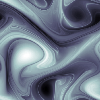
Figure 1: Snapshots of the vorticity field $\omega(x,y)$ at $t=61$ for the case $\mu(k>6)=0.1$ (upper) and at $t=65$ for the case $\mu(k>6)=0.2$ (lower) ($\mu=0.1$ for $k\leq 6$ for both cases). Light areas are regions of large positive values of the vorticity, and dark areas are regions of negative vorticity of large magnitude. The scales used in the two plots are not the same.

We note that the vorticity field for the case with a larger drag shows less fine structure and the large scale vortices tend to have shorter lifetime. At any given moment, there are typically 3 – 5 large vortex structures visible in the system. In the steady-state, vortices are continuously created and destroyed.

II Role of the finite-time Lyapunov exponent

II.1 Passive Nature of the Small-Scale Vorticity

The theory that we will use is based on the approximation that the high $k$ components of the vorticity field are passively advected by the large scale structures of the flow. This can be justified by the following argument given in Ref. Nam et al. (2000a). The Lyapunov exponent $h$ of the flow is the mean rate of exponentiation of differential displacement $\delta\vec{x}$ following the flow, where $d(\delta\vec{x})/dt=\delta\vec{x}\cdot\nabla\vec{v}$. Thus one can crudely estimate the Lyapunov exponent as

$$h\sim\langle\|\nabla\vec{v}\|^{2}\rangle^{\frac{1}{2}}\sim\sqrt{\int_{k_{f}}^{\infty}k^{2}E(k)dk}\ ,$$ (14)

where $\|\nabla\vec{v}\|^{2}=(\partial v_{x}/\partial x)^{2}+(\partial v_{y}/\partial y)^{2}+(\partial v_{x}/\partial y)^{2}+(\partial v_{y}/\partial x)^{2}$. Assuming the limit of infinite Reynolds number and power law behavior of $E(k)$ valid as $k\rightarrow\infty$, the integral in Eq. (14) diverges at the upper limit unless $\xi$ in Eq. (3) is positive. That is, the velocity field $\vec{v}$ is not differentiable ($h$ and $\nabla\vec{v}$ are undefined) unless $\xi>0$ (alternatively, if $\xi<0$ and viscosity imposes a cutoff to power law behavior of $E(k)$ at $k\sim k_{d}$, then, although $\|\nabla\vec{v}\|^{2}$ is now finite, the integral in Eq. (14) is dominated by velocity components at the shortest wavelength). From Eq. (14), for $\xi>0$, we have $h\sim k_{f}^{-\xi/2}$. This means that $h$, which characterizes small scale stretching, is determined by the largest scale flow components. Since $\xi>0$ in the case where drag is present, $\nabla\vec{v}$ is predominantly determined by the largest spatial scales. Thus the Lyapunov exponents provide information on the evolution of the distance between fluid elements whose separation is finite but small compared to $k_{f}^{-1}$. This will allow us to approximate the evolution of vorticity field components with wavenumbers in the range $k_{f}\ll k<k_{d}$ using Lyapunov exponents that result primarily from the large spatial scales $k\sim k_{f}$. That is, the vorticity field at wavenumber $k_{f}\ll k<k_{d}$ evolves via approximately passive advection by the large scale flow. (Note that for $\xi<0$ such an approach would not be applicable since the Lyapunov numbers would provide an estimate of separation evolution only for distances less that $k_{d}^{-1}$ which is outside the dissipationless power law range.)

Note that the case without drag corresponds to $\xi=0$, which is marginal in the sense that it is on the borderline of the condition for differentiability of the velocity field. In other situations of marginality (e.g., in critical phenomena), it is often found that there are logarithmic corrections to power-law scaling, and this may be thought of as the origin of Kraichnan’s logarithmic correction to the $k^{-3}$ enstrophy cascade scaling of $E(k)$.

II.2 Distribution of Finite-time Lyapunov Exponent

As mentioned earlier, the exponential divergence of nearby trajectories in a chaotic flow over a time interval $0$ to $t$ can be quantified by a finite-time Lyapunov exponent $h(t;\vec{x}_{0})$ defined in Eq. (13). In the limit $t\rightarrow\infty$, $h(t;\vec{x}_{0})$ will approach the usual infinite-time Lyapunov exponent $\bar{h}$ for almost all initial conditions $\vec{x}_{0}$ and almost all initial orientations of $\delta\vec{x}$. At finite time, the dependence of $h$ on $\vec{x}_{0}$ results in a distribution in the values of $h$ which can be characterized by the probability density function $P(h\,|\,t)$. That is, if $\vec{x}_{0}$ is chosen randomly with uniform density in the region of the fluid flow, and if the initial orientation of $\delta\vec{x}$ is arbitrarily chosen, then we can define a probability distribution $P(h\,|\,t)$ such that $P(h\,|\,t)dh$ is the probability that $h(t;\vec{x}_{0})$ lies between $h$ and $h+dh$. As $t$ increases, $P(h\,|\,t)$ will become more and more sharply peaked at $\bar{h}$ and approach a delta-function at $\bar{h}$ as $t\rightarrow\infty$.

The passive nature of the small-scale flow allows us to use the procedures described in Ref. Yuan et al. (2000) to obtain histogram approximations to $P(h\,|\,t)$. FIG. 2 shows $P(h\,|\,t)$ at different $t$ for the case of $\mu=0.2$.

Figure 2: Probability distribution function of the finite-time Lyapunov exponent $P(h\,|\,t)$ for different time $t$ for the case $\mu=0.2$.

As time increases, $P(h\,|\,t)$ becomes sharply peak around a positive value of $h$ showing that the flow is chaotic. In particular, for $t=20$, $P(h\,|\,t)$ has its peak at $\bar{h}\approx 0.20$. The function $P(h\,|\,t)$ shows similar behavior for the case $\mu=0.1$ with a peak occurring at $\bar{h}\approx 0.24$ for $t=20$. The smaller damping in the latter case apparently allows the fluid to undergo bigger stretching in a given amount of time.

Based on the argument that $h(t;\vec{x}_{0})$ can be considered as an average over many independent random realizations, $P(h\,|\,t)$ is approximated by the following asymptotic form (Ott (2002) and references therein),

$$P(h\,|\,t)\sim\sqrt{\frac{tG^{\prime\prime}(h)}{2\pi}}\,e^{-tG(h)}$$ (15)

for large $t$. Eq. (15) has been shown to be true for the generalized baker’s map Ott and Antonsen, Jr. (1989) and numerically verified for cases where there are no KAM surfaces, for example, see Ref. Városi et al. (1991). The function $G(h)$ is concave upward, $G^{\prime\prime}(h)\geq 0$. It has the minimum value zero, occurring at $h=\bar{h}$, $G^{\prime}(\bar{h})=G(\bar{h})=0$. The significance of Eq. (15) is that it expresses a function of two variables $P(h\,|\,t)$ in terms of a function of a single variable $G(h)$. Eq. (15) will be used in the development of the theory. We note that $G(h)$ is completely specified by the flow $\vec{v}(\vec{x},t)$ and hence, is dependent on the value of $\mu$.

The function $G(h)$ can be approximated at large $t$ from $P(h\,|\,t)$ using the following relation,

$$G(h)\approx K-\frac{1}{t}\ln P(h\,|\,t)\ ,$$ (16)

where $K$ is determined by the condition that the minimum of $G(h)$ equals zero. FIG. 3 shows the $G(h)$ obtained from the corresponding $P(h\,|\,t)$ shown in FIG. 2.

Figure 3: $G(h)$ (see Eq. (15)) for different time $t$ for the case $\mu(k>6)=0.2$. The inset shows $G(h)$ obtained at $t=20$ (solid line) and the quadratic approximation to $G(h)$ obtained by the method described at the end of Sec. III.2 (dashed line).

The large number $(4096^{2})$ of fluid trajectories used in the generation of each $P(h\,|\,t)$ allows us to obtain $G(h)$ for a large range of $h$. As can be seen in FIG. 3, for large enough $t$, the graphs of $G(h)$ for different $t$ more or less collapse onto each other, showing that Eq. (15) is a good approximation to $P(h\,|\,t)$ for the flows we considered. $G(h)$ shows similar behavior in the case $\mu=0.1$.

III The Exponents $\xi$ and $\zeta_{2q}$

III.1 Review of Theory

We consider the scaling of the vorticity structure functions in the limit $\nu\rightarrow 0^{+}$. The results have previously been given in Ref. Neufeld et al. (2000); Chertkov (1998), which treats finite-lifetime passive scalars Abraham (1998); Chertkov (1998); Nam et al. (1999) rather than vorticity in two-dimensional turbulence with drag, and in Ref. Boffetta et al. (2002) for two-dimensional turbulence with drag. Here, we re-derive the previous results (our derivation is different from that in Ref. Neufeld et al. (2000); Chertkov (1998) and more complete than that in Ref. Boffetta et al. (2002)).

From Eq. (2) with initial condition $\omega(\vec{x},0)=0$, we have Neufeld et al. (2000),

$$\delta_{\vec{r}}\omega(\vec{x},t) = \int_{0}^{t}\delta f_{\omega}[\vec{x}(t^{\prime})]e^{\mu(t-t^{\prime})}dt^{\prime}$$ (17)

$$\sim \int_{t-\tau(r)}^{t}\vec{r}\cdot\nabla f_{\omega}[\vec{x}(t^{\prime})]e^{(\mu-h)(t^{\prime}-t)}dt^{\prime}$$

$$+\ \int_{0}^{t-\tau(r)}\delta f_{\omega}[\vec{x}(t^{\prime})]e^{\mu(t^{\prime}-t)}dt^{\prime}\ .$$

where $\delta f_{\omega}[\vec{x}(t^{\prime})]=f_{\omega}[\vec{x}(t^{\prime})+\delta\vec{x}(t^{\prime})]-f_{\omega}[\vec{x}(t^{\prime})]$, $\vec{x}(t^{\prime})$ and $\vec{x}(t^{\prime})+\delta\vec{x}(t^{\prime})$ are the two trajectories that pass through $\vec{x}$ and $\vec{x}+\vec{r}$ at $t^{\prime}=t$; thus $\delta\vec{x}(t)\equiv\vec{r}$. Since the points $\vec{x}$ and $\vec{x}+\vec{r}$ are specified at time $t$, chaos in the flow implies that the backward evolved trajectories to times $t^{\prime}<t$ diverge exponentially from each other, $\delta\vec{x}(t^{\prime})\sim\vec{r}e^{h(t-t^{\prime})}$, until $|\delta\vec{x}(t^{\prime})|$ reaches the system size $L$, past which $|\delta\vec{x}(t^{\prime})|$ remains of order $L$. We define $\tau(r)$ such that $|\delta\vec{x}(t-\tau)|\sim L\sim re^{h\tau}$. We have linearized $\delta f_{\omega}[\vec{x}(t^{\prime})]$ for $t-\tau(r)<t^{\prime}<t$ when the two trajectories are close together. On the other hand, for $0<t^{\prime}<t-\tau(r)$, $|\delta\vec{x}(t^{\prime})|\sim L$ and $\delta f_{\omega}[\vec{x}(t^{\prime})]$ thus fluctuates with roughly constant amplitude, $\delta f_{\omega}\sim f_{\omega}$. Thus the integral from 0 to $t-\tau(r)$ in Eq. (17) is of the order of $e^{-\mu\tau}$ Boffetta et al. (2002). The integral from $t-\tau(r)$ to $t$ in Eq. (17) shows the same $\sim e^{-\mu\tau}$ behavior if $h>\mu$ but is of the order of $e^{-h\tau}$ if $h<\mu$. Hence, using the definition of $S_{2q}(r)$ and replacing the average over $\vec{x}$ by an average over $\tau$ at fixed exponentiation $\lambda=\ln(L/r)=h\tau$, we find

$$S_{2q}(r)\sim\int_{0}^{\frac{\lambda}{\mu}}\!d\tau\,R(\tau\,|\,\lambda)e^{-2q\mu\tau}+\int_{\frac{\lambda}{\mu}}^{\infty}\!d\tau\,R(\tau\,|\,\lambda)e^{-2q\lambda}\ .$$ (18)

The conditional probability density $R(\tau\,|\,\lambda)$ of $\tau$ for a fixed $\lambda$ is related to $P(h\,|\,\tau)$ by Reyl et al. (1998)

$$R(\tau\,|\,\lambda)\approx\frac{d}{d\tau}\int_{\frac{\lambda}{\tau}}^{\infty}\!dh\,P(h\,|\,\tau)\ .$$ (19)

Using the asymptotic form Eq. (15) for $P(h\,|\,\tau)$, the integral Eq. (18) is performed using the steepest descent method with $\lambda$ as the large parameter. Thus we obtain that the structure function scaling exponents, $\zeta_{2q}$ defined in Eq. (4), is given by

$$\zeta_{2q}=\displaystyle\min_{h}\{2q,H_{q}(h)\}\ ,$$ (20)

where

$$H_{q}(h)=\frac{G(h)+2q\mu}{h}\ .$$ (21)

Equations (20) and (21) yield the previous passive scalar result of Ref. Chertkov (1998) if $G(h)$ is assumed parabolic, $G(h)=(constant)(h-\bar{h})^{2}$, which is a consequence of the temporally white noise velocity field model of Ref. Chertkov (1998).

We now consider the energy density $e(\vec{k})$ which is given by

$$e(\vec{k})=\frac{1}{(2\pi)^{2}}\frac{|\tilde{v}_{x}(\vec{k})|^{2}+|\tilde{v}_{y}(\vec{k})|^{2}}{2L^{2}}\,,$$ (22)

where $\tilde{v}_{x}(\vec{k})$ and $\tilde{v}_{y}(\vec{k})$ are Fourier transforms of the $x$ and $y$ components of the velocity field $\vec{v}(x,y)$. The wavenumber energy spectrum $E(k)$ is then defined as

$$E(k)=\int d\vec{k}^{\prime}\delta(|\vec{k}^{\prime}|-k)e(\vec{k}^{\prime})\,.$$ (23)

A previous theory Nam et al. (2000a, b) relates the energy wavenumber spectrum exponent, $\xi$ defined in Eq. (3) to $G(h)$. The result is

$$\xi=\min_{h}\{H_{1}(h)\}\ .$$ (24)

Thus, $\xi$ and $\zeta_{2q}$ are related to the properties of the flow, namely the drag coefficient $\mu$ and the distribution of the finite-time Lyapunov exponent $h$.

Let $h=h_{q}^{*}$ be the value of $h$ at which $H_{q}(h)$ is minimum. We now show that $h_{q}^{*}$ increases with $q$. Letting $\beta>\alpha$, by the definition of $h_{q}^{*}$, $H^{\prime}_{\alpha}(h_{\alpha}^{*})=H^{\prime}_{\beta}(h_{\beta}^{*})=0$, it follows that $G^{\prime}(h_{\beta}^{*})-H_{\beta}(h_{\beta}^{*})=G^{\prime}(h_{\alpha}^{*})-H_{\alpha}(h_{\alpha}^{*})$. Since by Eq. (21), $H_{\beta}(h)>H_{\alpha}(h)$ for all $h$, we have $G^{\prime}(h_{\beta}^{*})>G^{\prime}(h_{\alpha}^{*})$ which implies $h_{\beta}^{*}>h_{\alpha}^{*}$ due to the fact that $G^{\prime\prime}(h)>0$ for all $h$. Moreover, putting $\alpha=0$ gives $h_{q}^{*}>\bar{h}$ for all $q$.

III.2 Comparison of Theory and Numerical Results

To apply the theory Eq. (20) and Eq. (24) to numerically determine the exponents $\zeta_{2q}$ and $\xi$ of our turbulent flow governed by Eq. (2), we first let

$$\bar{\zeta}_{2q}=\min_{h}\{H_{q}(h)\}\ .$$ (25)

Using Eq. (21), we re-write Eq. (25) as

$$\min_{h}\left\{\frac{G(h)+2q\mu}{h}-\bar{\zeta}_{2q}\right\}=0\ .$$ (26)

Since the function minimized in Eq. (26) has minimum value zero, we can multiply it by any positive function of $h$, and the minimum will still be zero. Thus for $h>0$ we can multiply the minimized function by $h$ to obtain

$$\min_{h}\{G(h)-h\bar{\zeta}_{2q}\}=-2q\mu\ .$$ (27)

Using Eq. (15) and Eq. (27), we see that steepest descent evaluation of the following integral for large $t$ yields

$$\int P(h\,|\,t)e^{h\bar{\zeta}_{2q}t}\,dh\sim e^{2q\mu t}\ .$$ (28)

Thus we define the partition function Reyl et al. (1998)

$$\Gamma(z,t)=\int e^{zh(t;\vec{x}_{0})t}\,d\vec{x}_{0}\ ,$$ (29)

in terms of which Eq. (28) becomes

$$\Gamma(\bar{\zeta}_{2q},t)\sim e^{2q\mu t}\ .$$ (30)

We numerically compute the partition function Eq. (29) using the approximation,

$$\Gamma(z,t)=\frac{1}{M}\sum_{i=1}^{M}\,e^{zh(t;\vec{x}_{0i})t}$$ (31)

employing many ($M$=$4096^{2}$) spatially uniformly distributed initial conditions $\vec{x}_{0i}$ $(i=1,2,\ldots,M)$.

For different values of $\bar{\zeta}_{2q}$, we then plot $\ln\Gamma(\bar{\zeta}_{2q},t)$ versus $t$. FIG. 4 shows samples of $\ln\Gamma(\bar{\zeta}_{2q},t)$ for the case $\mu=0.1$.

Figure 4: Log-linear plot of the partition function $\Gamma(\bar{\zeta}_{2q},t)$ for $\mu=0.1$. The dotted lines are linear fits.

As expected, for large $t$, $\ln\Gamma(\bar{\zeta}_{2q},t)$ is linear in $t$ and the slope, which can be estimated using a linear fit, gives the corresponding value of $q$ for each $\bar{\zeta}_{2q}$. FIG. 5 plots $\bar{\zeta}_{2q}$ versus $q$ obtained in this way for $\mu=0.1$ and $\mu(k>6)=0.2$ (open circles and squares) together with the corresponding sixth degree polynomial fits (solid lines).

Figure 5: $\bar{\zeta}_{2q}$ as a function of $q$ from the method of FIG. 4 for $\mu=0.1$ (circle) and $\mu(k>6)=0.2$ (square). The solid lines are sixth degree polynomial fits to circles and squares. Results using Eq. (5) of Ref. Chertkov (1998) are shown as dashed lines.

By Eq. (24) and Eq. (20), the exponents $\xi$ and $\zeta_{2q}$ can then be determined from FIG. 5 by $\xi=\bar{\zeta}_{2}$ and $\zeta_{2q}=\min\{2q,\bar{\zeta}_{2q}\}$.

It is also possible to compute $\xi$ and $\zeta_{2q}$ directly from Eq. (24) and Eq. (20) using a fourth degree polynomial fit of the numerically obtained $G(h)$. We find that the two methods give similar results, but that the method of Eq. (31) is easier to compute.

We also test the applicability of the result of Ref. Chertkov (1998), which employs a model in which the velocity field is $\delta$-correlated in time. This model may be shown to correspond to Eq. (20) and Eq. (21) with $G(h)$ parabolic, $G(h)=a(h-\bar{h})^{2}$ where $\bar{h}$ is the infinite time Lyapunov exponent. With this form of $G(h)$, an explicit analytic expression for the structure function exponents can be obtained in terms of the constant $a$ and $\bar{h}$; see Eq. (5) of Ref. Chertkov (1998). In order to apply this result to a specific flow, we need to formulate a procedure for obtaining a reasonable value of $a$ from the flow ($\bar{h}$ is well-defined and numerically accessible by standard technique). For this purpose, we note that, within the $\delta$-correlated approximation, the total exponentiation $h(t,\vec{x}_{0})t$ experienced by an infinitesimal vector originating at position $\vec{x}_{0}$ undergoes a random walk with diffusion constant $D=a/4$. Thus we obtain $a$ as one half of the long time slope of a plot of $\langle(h-\bar{h})^{2}\rangle t^{2}$ versus $t$. The inset to FIG. 3 shows as a solid curve $G(h)$ obtained using Eq. (16) (as previously described) along with the parabolic model (dashed curve) with $a$ determined by the above procedure. There appears to be a substantial difference in the important range $h>\bar{h}$ where the saddle points are located. Somewhat surprisingly, however, this does not lead to much difference in the numerical values of the structure function exponents. This is shown in FIG. 5 where the results using Eq. (5) of Ref. Chertkov (1998) are plotted as dashed curves. In fact, the difference is within the error of our numerical experiments that directly determine the values of $\zeta_{2q}$. Thus for this case the parabolic approximation provides an adequate fit to the data, although this could not be definitely predicted a priori.

III.2.1 Energy Wavenumber Spectrum

As illustrated in FIG. 5, theoretical predictions for $\xi$, denoted as $\xi_{th}$, are obtained using the method described above. The results are given in TABLE 1.

Table 1: Comparison of the values of $\xi$ obtained from numerical simulations to the theoretical results.

$\mu(k>6)$	$\xi_{th}(=\zeta_{2,th})$	$\xi_{DNS}$	$\zeta_{2,DNS}$	$\zeta_{2,E(k)}$
0.1	0.63	0.61	0.66	0.68
0.2	1.10	1.12	1.16	1.14

To verify the theoretical results, we compute the energy spectrum directly from the numerical solution of Eq. (2) on a $4096\times 4096$ grid using Eq. (23), which can be written in terms of the vorticity as

$$E(k,t)=\int\frac{d\vec{k}^{\prime}}{(2\pi L)^{2}}\,\delta(|\vec{k}^{\prime}|-k)\frac{|\tilde{\omega}(\vec{k}^{\prime},t)|^{2}}{2|\vec{k}^{\prime}|^{2}}$$ (32)

where $\tilde{\omega}(\vec{k}^{\prime},t)$ is the Fourier transform of $\omega(\vec{x},t)$. The time averaged energy spectrum $E(k)$ is obtained by averaging $E(k,t)$ at every 0.1 time unit from $t=41$ to $t=75$. FIG. 6 shows a log-log plot of $E(k)$ versus $k$ for the two

Figure 6: Energy wavenumber spectra. The dotted lines are the corresponding linear fit in the scaling range.

different values of $\mu(k>6)$ we considered. In both cases, a clear scaling range of more than a decade can be observed. We measure the scaling exponents by linearly fitting $E(k)$ in the scaling range. The results, denoted $\xi_{DNS}$, are shown in TABLE 1. Good agreement is found between the numerical and the theoretical results. These results are consistent with those of previous work in Nam et al. (2000a) and Boffetta et al. (2002) which use grids of $1024\times 1024$ and $2048\times 2048$, respectively.

III.2.2 Vorticity Structure Functions

Numerical tests of theoretical predictions of structure function exponents of finite-lifetime passive scalar fields advected by simple chaotic flows have been performed in Ref. Neufeld et al. (2000) and Boffetta et al. (2002). To test the analogous theoretical predictions, Eq. (20) and Eq. (21), in the case of two-dimensional turbulence with drag, we define the averaged structure functions of order $2q$ as

$$S_{2q}(r)=\int\frac{d\vec{r}\,^{\prime}}{2\pi r}\delta(r-|\vec{r}\,^{\prime}|)\langle\,|\delta_{\vec{r}^{\prime}}\omega|^{2q}\rangle\ .$$ (33)

The angled brackets denote average over the entire region occupied by the fluid. The angular dependence of $\langle\,|\delta_{\vec{r}^{\prime}}\omega|^{2q}\rangle$ is averaged out in Eq. (33) by the integration over $\vec{r}\,^{\prime}$. Using Eq. (33) with $\omega(\vec{x},t)$ obtained from the numerical integration of Eq. (2), we compute $S_{2q}(r)$ from $t=41$ to $t=75$ at every 1 time unit and take the average of the results obtained.

Following the scheme described above, we calculate the time-averaged structure functions for $q$ ranging from 0.0 to 2.0. FIGS. 7(a) and 8(a) show samples of the results for the cases $\mu=$0.1 and 0.2, respectively. The distance $r$ is measured in the unit of grid size.

Figure 7: For the case of $\mu=0.1$: (a) structure functions of vorticity difference, for various orders $q$ between 0.1 and 2.0; the dotted lines are linear fits in the scaling range. (b) Plot of $\zeta_{2q}/\zeta_{2}$ obtained from numerical simulations (circle) and from Eq. (20) (cross), for different values of $q$; the solid lines are polynomial fits to the circles and the crosses (cf. Eq. (54)).

Figure 8: For the case of $\mu=0.2$: (a) structure functions of vorticity difference, for various orders $q$ between 0.1 and 2.0; the dotted lines are linear fits in the scaling range. (b) Plot of $\zeta_{2q}/\zeta_{2}$ obtained from numerical simulations (circle) and from Eq. (20) (cross), for different values of $q$; the solid lines are polynomial fits to the circles and the crosses (cf. Eq. (54)).

For all values of $q$ we have studied, the structure functions show a clear scaling range that is long enough to allow an estimate of the scaling exponents, $\zeta_{2q}$. The scaling range of the structure functions in real space roughly corresponds to that of the energy spectrum in $k$-space. The values of $\zeta_{2q}$ are obtained by measuring the slope of the structure functions in the scaling range using a linear fit. Results for $\zeta_{2q}/\zeta_{2}$ are shown as circles in FIGS. 7(b) and 8(b). The measured values of $\zeta_{2}$, denoted as $\zeta_{2,DNS}$, are given in TABLE 1. We then obtain theoretical predictions to $\zeta_{2q}$ from the polynomial fit of $\bar{\zeta}_{2q}$ shown in FIG. 5, following procedures described at the beginning of this section. The results are shown as crosses in FIG. 7(b) and 8(b) for the two cases of $\mu$ we studied. The predicted values of $\zeta_{2}$, denoted as $\zeta_{2,th}$, are given in TABLE 1. The numerical and theoretical results agree reasonably well for all $q$’s. In reference to Eq. (20) we note that, for all the cases we numerically tested, we found that $\zeta_{2q}=\bar{\zeta}_{2q}<2q$ for all $q$. This is consistent with the general result that for $\mu<\bar{h}$, $\bar{\zeta}_{2q}<H_{q}(\bar{h})<2q$. We note, however, that this need not hold in general, particularly for large $\mu$.

III.3 Discussion

III.3.1 Energy Wavenumber Spectrum

The presence of drag gives a power law for the energy spectrum that falls faster than the case without drag and $\xi$ is the correction to the classical zero drag value of the scaling exponent. Note that the major contribution to the integrals involved in the theory Nam et al. (2000b) comes from the immediate neighborhood of $h=h_{1}^{*}$, where $h_{1}^{*}$ is the value of $h$ at which the minimum of $H_{1}(h)$ occurs. As $\mu\rightarrow 0$, $h_{1}^{*}\rightarrow\bar{h}$ and hence $\xi\rightarrow 0$. The scaling exponent is thus determined by the majority of fluid trajectories with stretching rate close to $\bar{h}$. On the other hand, for $\mu\neq 0$, $h_{1}^{*}>\bar{h}$. Therefore the scaling exponent is determined by a small number of fluid trajectories that experience a stretching rate $h_{1}^{*}$, that is larger than the typical stretching rate $\bar{h}$, and $h_{1}^{*}$ increases with $\mu$ ($h_{1}^{*}$ for $\mu=0.1$ and $\mu=0.2$ are 0.47 and 0.57 respectively). The reason for this, and in general $h^{*}_{q}>\bar{h}$ as we have shown in Section III.1, is that the presence of drag introduces the exponential decaying factor $e^{-\mu\tau}$ in Eq. (18) and the corresponding integral for $E(k)$ Nam et al. (2000b). Thus, for a certain fixed $k$ (or $\lambda$), the fluid trajectories that contribute most to $E(k)$ (or $S_{2q}(r)$) are those with smaller $\mu\tau$, and hence larger stretching rate $h$.

It should also be clear from the above discussion that, in order to get an accurate estimate to $\xi$, it is important to take into account the fluctuation in the finite-time Lyapunov exponent. If we were to neglect the fluctuation and take the stretching rate to be $\bar{h}$ for all trajectories, we would have overestimate $\xi$ to be $2\mu/\bar{h}$.

III.3.2 Vorticity Structure Functions

The theory predicts that when drag is present, an inertial range exists in which the vorticity structure functions $S_{2q}(r)$ exhibit power-law scaling. The scaling exponent $\zeta_{2q}$ is given by Eq. (20). In the absence of intermittency $\zeta_{2q}$ scales linearly with $q$ and $\zeta_{2q}/\zeta_{2}=q$, which is plotted as the straight dashed line in FIGS. 7(b) and 8(b). For $\mu>0$, Eq. (20) predicts that $\zeta_{2q}$ varies nonlinearly with $q$, as shown in FIGS. 7(b) and 8(b). This anomalous scaling of $S_{2q}(r)$, which indicates the presence of intermittency in the system, is verified numerically in both cases.

The anomalous scaling of $S_{2q}(r)$ is the result of the combined effect of drag and non-uniform stretching of fluid elements. If all fluid elements have the same stretching rate, say $\bar{h}$, then $e^{-\mu\tau}$ becomes a constant and thus $\zeta_{2q}$ is proportional to $2q$. On the other hand, if $\mu=0$, regardless of whether the stretching is uniform or not, $\zeta_{2q}=0$. FIGS. 7(b) and 8(b) also suggest that $S_{2q}(r)$ shows larger deviation from the simple scaling behavior, $\zeta_{2q}/\zeta_{2}=q$, as $\mu$ increases.

We remark that the statistical error in the predictions of the values of the higher order structure function scaling exponents is in general larger. This is because, as already mentioned in Section III.1, $h_{q}^{*}$ increases with $q$, hence for large $q$, $\zeta_{2q}$ depends mostly on a rare number of fluid trajectories with large $h$.

III.3.3 $S_{2}(r)$ and $E(k)$

We now focus on the second order structure function $S_{2}(r)$. With the isotropic assumption, the following relation between $S_{2}(r)$ and $E(k)$ can be obtained,

$$S_{2}(r)=4\int\!dk\,[1-J_{0}(kr)]k^{2}E(k)$$ (34)

where $J_{0}$ is the zeroth order Bessel function of the first kind. We compute $S_{2}(r)$ by Eq. (34) using the $E(k)$ shown in FIG. 6. The results are plotted as solid lines in FIG. 9,

Figure 9: Second order structure functions $S_{2}(r)$ obtained from the energy spectrum $E(k)$ using Eq. (34) (solid line with circles) and from direct numerical simulations (dotted line).

the scaling exponents, denoted as $\zeta_{2,E(k)}$, are then measured and compared with $\zeta_{2,DNS}$ in TABLE 1. The $S_{2}(r)$ obtained directly from Eq. (33) are plotted as dashed lines in the same diagram for comparison. Ignoring viscosity at the small scales and forcing at the large scales, we can assume $E(k)\sim k^{-(3+\xi)}$ for all $k$. Then it follows from Eq. (34) that, for $0<\xi<2$, $S_{2}(r)\sim r^{\zeta_{2}}$ for all $r$ and $\zeta_{2}=\xi$. This is consistent with our theory which predicts that $\zeta_{2,th}=\xi_{th}$ when $0<\zeta_{2,th}<2$. Comparing $\zeta_{2,DNS}$ to $\xi_{DNS}$, we find reasonably good agreements but we note that $\zeta_{2,DNS}$ is in general slightly larger than $\xi_{DNS}$. We shall see that this small discrepancy is a result of the dependence of $S_{2}(r)$ on the large scales of the flow.

Due to the effects of forcing and viscosity, $E(k)$ deviates from the power-law behavior at very small and very large $k$. According to Eq. (34), these deviations will affect $S_{2}(r)$. This is demonstrated in FIG. 10 in which we plot the $S_{2}(r)$ calculated by Eq. (34) using three different $E(k)$.

Figure 10: Second order structure functions $S_{2}(r)$ calculated by Eq. (34) using different $E(k)$: pure power law (cross), power law with small scales viscous cutoff (circle) and power law with large scales fluctuations (square). The inset shows the different $E(k)$ versus $k$ with corresponding labels.

The first one is a pure power law for all $k$. The second one is the same as the first one except it drops faster at large $k$ mimicking the viscous cutoff. The third one is constructed from the first one by modifying the first five modes to mimic the presence of large scale forcing. The range of $k$ used corresponds to a $1024\times 1024$ lattice. From FIG. 10, it is seen that while the viscous effect is negligible except at small $r$, the large scale forcing can have a significant effect on the general shape of $S_{2}(r)$. As a result, $S_{2}(r)$ may have a very limited scaling range even when $E(k)$ shows a reasonably long one. We believe this is generally true for structure functions of any order, making it more difficult to accurately measure $\zeta_{2q}$ than $\xi$. We are able to obtain reliable estimates of $\zeta_{2q}$, as verified by the agreement between $\zeta_{2,DNS}$ and $\xi_{DNS}$, by employing a $4096\times 4096$ lattice and the time-averaging process.

IV Probability Distribution of Vorticity Difference

IV.1 Theory

In this section, we shall derive an expression for the probability distribution function $P_{r}(\delta_{\vec{r}}\omega)$ of the vorticity difference $\delta_{\vec{r}}\omega$ in terms of the conditional probability density function $R(\tau\,|\,\lambda)$. In Section III.1, we introduced $R(\tau\,|\,\lambda)$ and deduced the scaling of $\delta_{\vec{r}}\omega$ by doing order of magnitude estimations of the integrals in Eq. (17). We now determine the distribution of $\delta_{\vec{r}}\omega$ by estimating the values of these integrals for different fluid trajectories. We shall assume the system is isotropic so that $P_{r}(\delta_{\vec{r}}\omega)$ depends on the distance $r$ only, and not on the direction of $\vec{r}$.

Referring to Eq. (17), for $t-\tau<t^{\prime}<t$, we estimate that $\vec{r}\cdot\nabla f_{\omega}[\vec{x}(t^{\prime})]\sim(r/L)f_{\omega}[\vec{x}(t^{\prime})]=e^{-\lambda}f_{\omega}[\vec{x}(t^{\prime})]$. For $0<t^{\prime}<t-\tau$, the separation between the two trajectories is of order $L$ and the values of $f_{\omega}[\vec{x}(t^{\prime})]$ along the two trajectories become uncorrelated, hence $\delta f_{\omega}[\vec{x}(t^{\prime})]\sim f_{\omega}[\vec{x}(t^{\prime})]$. Approximating $f_{\omega}[\vec{x}(t^{\prime})]$ as varying randomly, the values of the first and the second integral in Eq. (17) are respectively estimated as $[f_{\omega}/(\mu-h)](e^{-\lambda}-e^{-\mu\tau})$ and $(f_{\omega}/\mu)e^{-\mu\tau}$. This suggests that we can treat $\delta_{\vec{r}}\omega$ as a function of two random variables $\tau$ and $Z=f_{\omega}/\mu$ as follow,

$$\delta_{\vec{r}}\omega(Z,\tau)\approx Z\,\frac{e^{-\lambda}+e^{-\mu\tau}}{2}\ .$$ (35)

We then write the probability distribution function of $\delta_{\vec{r}}\omega$ as,

$$P_{r}(\delta_{\vec{r}}\omega)=\int_{0}^{\infty}P_{r}(\delta_{\vec{r}}\omega|\tau)R(\tau\,|\,\lambda)\,d\tau$$ (36)

where $P_{r}(\delta_{\vec{r}}\omega|\tau)$ is the conditional probability distribution function of $\delta_{\vec{r}}\omega$ given $\tau$. From Eq. (35) and letting $y(\tau)=(e^{-\lambda}+e^{-\mu\tau})/2$, we have,

$$P_{r}(\delta_{\vec{r}}\omega|\tau)=\frac{1}{y(\tau)}P_{Z}\left[\frac{\delta_{\vec{r}}\omega}{y(\tau)}\right]$$ (37)

where $P_{Z}$ is the probability density function of $Z$. Note that when $r=L$, $\lambda=\tau=0$, which implies $\delta_{\vec{r}}\omega|_{r=L}=Z$. Therefore, we obtain the result,

$$P_{r}(\delta_{\vec{r}}\omega)=\int_{0}^{\infty}\frac{1}{y(\tau)}P_{L}\left[\frac{\delta_{\vec{r}}\omega}{y(\tau)}\right]R(\tau\,|\,\lambda)\,d\tau\ .$$ (38)

Reference Chertkov (1998) has previously derived the probability distribution function for differences of finite lifetime passive scalars advected by a temporally white noise model velocity field. For the model used in Ref. Chertkov (1998) the difference probability distribution function at large separation $|\vec{r}|$ is Gaussian, while this is not the case for our flow. In order to obtain reasonable agreement between the theory Eq. (38) and our numerical experiments, it is important to account for the non-Gaussian behavior of the probability distribution function of the vorticity difference at large separation $|\vec{r}|$. In what follows, this will be done by using the numerically obtained probability distribution function at large $|\vec{r}|$ as an input to Eq. (38) to determine the probability distribution function at small $|\vec{r}|$.

IV.2 Comparison of Theory and Numerical Results

We first compute the probability distribution function $\bar{P}_{r}(X_{\vec{r}})$ of the standardized vorticity difference $X_{\vec{r}}$, Eq. (5), directly from the numerical solution of Eq. (2). The vorticity field $\omega(\vec{x},t)$ from $t=41$ to $t=75$ at every 1 time unit is used in this computation. The separating distance $\vec{r}$ is taken to be in the $\hat{x}$-direction and is measured in the unit of grid size. For $\mu=0.1$, the results for four different values of $r$ are shown as solid lines in FIG. 11.

Figure 11: For $\mu=0.1$, the probability distribution function $\bar{P}_{r}(X_{\vec{r}})$ of the standardized vorticity difference $X_{\vec{r}}$ obtained from direct numerical simulation (solid lines) and from Eq. (38) (dashed lines). The separating distance $\vec{r}$ is in the $\hat{x}$-direction and measured in the unit of grid size.

It is clear that the shape of $\bar{P}_{r}(X_{\vec{r}})$ changes as $r$ varies in the range $4\leq r\leq 512$, indicating the system is intermittent. $\bar{P}_{r}(X_{\vec{r}})$ develops exponential tails (e.g., $r=64$) and then stretched-exponential tails (e.g., $r=4$) as $r$ decreases. We note that $\bar{P}_{r}(X_{\vec{r}})$ for all $r\leq 4$ collapse onto each other, and similarly, all the $\bar{P}_{r}(X_{\vec{r}})$ with $r\geq 512$ have the same shape. Numerical results similar to those in FIG. 11 have also been obtained in Ref. Boffetta et al. (2002), but theory for $\bar{P}_{r}(X_{\vec{r}})$ was not presented in Ref. Boffetta et al. (2002).

To apply the theoretical result Eq. (38), we first derive an expression for $R(\tau\,|\,\lambda)$. To this end, we approximate $G(h)$ as a quadratic function of $h$,

$$G(h)\approx a(h-\bar{h})^{2}\ .$$ (39)

Using the relation Eq. (19) and the asymptotic form for $P(h\,|\,t)$, Eq. (15), we obtain

$$R(\tau\,|\,\lambda) = \frac{\lambda}{2\tau^{2}}P(h=\frac{\lambda}{\tau}\,|\,\tau)$$ (40)

$$\sim \frac{1}{2}\sqrt{\frac{a}{\pi\tau}}\left(\frac{\lambda}{\tau}-\bar{h}\right)e^{-\tau a\left(\frac{\lambda}{\tau}-\bar{h}\right)^{2}}\ .$$

To compare the predictions by Eq. (38) with numerical results, the $G(h)$ for $\mu=0.1$ is obtained numerically as described in Section II.2 and fitted to Eq. (39) in the vicinity of its minimum to obtain the parameters $a$ and $\bar{h}$. This quadratic fit is a good approximation because the integral in Eq. (38) is dominated by the region where $R(\tau\,|\,\lambda)$ is large, which roughly corresponds to the region where $P(h\,|\,t)$ is maximum. FIG. 12 shows the $R(\tau\,|\,\lambda)$ for $\mu=0.1$ obtained using

Figure 12: For $\mu=0.1$, the conditional probability density function $R(\tau\,|\,\lambda)$ given by Eq. (40) ($a=1.55$, $\bar{h}=0.26$) for different values of $\lambda$.

the quadratic approximation Eq. (39). We then take $P_{L}$ in Eq. (38) to be of the form $\exp(W)$ where $W$ is an even sixth degree polynomial fitted to the numerically computed $\ln[P_{r}(\delta_{\vec{r}}\omega)]$ for $\vec{r}=1024\hat{x}$ and $\mu=0.1$. With $R(\tau\,|\,\lambda)$ and $P_{L}$ obtained as described above, we compute $P_{r}(\delta_{\vec{r}}\omega)$, and thus $\bar{P}_{r}(X_{\vec{r}})$, for different values of $r$ using Eq. (38). The results are plotted as dashed lines in FIG. 11. The theoretical predictions agree well with the numerical results. We also find good agreements between our theory and numerical simulations when $\vec{r}$ is taken to be in the $\hat{y}$-direction. Similar results were also obtained for the case $\mu(k>6)=0.2$.

IV.3 Discussion

According to Eq. (38), $P_{r}(\delta_{\vec{r}}\omega)$ for a given $r$ can be considered as a superposition of many different probability distribution functions, each obtained by rescaling $P_{L}(\delta_{\vec{r}}\omega)$ to a different width using $y(\tau)$. The amplitude of each component is then determined by the coefficient $R(\tau\,|\,\lambda)$. Since the statistics between two points separated by distance $r\sim L$ are uncorrelated, the distribution $P_{L}(\delta_{\vec{r}}\omega)$ is virtually the one-point probability distribution of the vorticity $\omega$, which is not necessarily Gaussian and is closely related to the statistics of the source $f_{\omega}$, as implied by the definition of $Z$. Hence, Eq. (38) relates the distribution of the vorticity difference to the one-point statistics of the source.

As can be seen in FIG. 12, $R(\tau\,|\,\lambda)$ has a very sharp peak when $\lambda$ is small ($r$ is large). Thus, only a small range of values of $\tau$ contributes to the integral Eq. (38). This gives the expected result that $P_{r}(\delta_{\vec{r}}\omega)$ has similar shape as $P_{L}(\delta_{\vec{r}}\omega)$ when $r$ is large. As $\lambda$ increases ($r$ decreases), the width of $R(\tau\,|\,\lambda)$ increases. According to Eq. (38), $P_{r}(\delta_{\vec{r}}\omega)$ is now composed of a large number of rescaled $P_{L}(\delta_{\vec{r}}\omega)$ with a broad range of width. This gives rise to the broader-than-Gaussian tails in $P_{r}(\delta_{\vec{r}}\omega)$ for small $r$.

Like the anomalous scaling of the vorticity structure functions, the dependence of the shape of $P_{r}(\delta_{\vec{r}}\omega)$ on $r$ is a result of the presence of drag and the non-uniform stretching of fluid elements. If $h=\bar{h}$ for all fluid trajectories, then $R(\tau\,|\,\lambda)=\delta(\tau-\lambda/\bar{h})$, and from Eq. (38), $P_{r}(\delta_{\vec{r}}\omega)$ has the same form for all $r$, indicating a self-similar flow. On the other hand, if $\mu=0$, $y(\tau)$ becomes independent of $\tau$, which also implies $P_{r}(\delta_{\vec{r}}\omega)$ is independent of $r$. In both situations, $P_{r}(\delta_{\vec{r}}\omega)$ will have the same shape as $P_{L}(\delta_{\vec{r}}\omega)$.

We remark that while the width of the distribution $P_{r}(\delta_{\vec{r}}\omega)$ in Eq. (38) depends precisely on the choice of the value for the multiplicative constant on the right hand side of Eq. (35), our results for $\bar{P}_{r}(X_{\vec{r}})$ are independent of this value.

V Multifractal Formulation

V.1 Theory

The local viscous energy dissipation rate per unit mass $\varepsilon$ and its global average value $\langle\varepsilon\rangle$ play important roles in the phenomenology of three-dimensional turbulence Stolovitzly and Sreenivasan (1994). It is now well known that $\varepsilon$ shows intermittent spatial fluctuations which can be described by the multifractal formulation Frisch (1995). Using the measure $p^{\prime}(r)=\mathcal{E}_{r}/\mathcal{E}$, where $\mathcal{E}_{r}$ is the total dissipation in a volume of linear dimension $r$ and $\mathcal{E}$ is the total dissipation in the whole domain, the Rényi dimension spectrum $D_{q}$ and the singularity spectrum $f(\alpha)$ have been measured experimentally Chhabra et al. (1989); Meneveau and Sreenivasan (1991).

Intermittency in three-dimensional turbulence also manifests itself as anomalous scaling in the velocity structure functions $S^{\prime}_{3q}(r)$ defined as

$$S^{\prime}_{3q}(r)=\langle(\delta_{\vec{r}}v)^{3q}\rangle\sim r^{\zeta^{\prime}_{3q}}\ ,$$ (41)

where $v$ is the component of the velocity vector in the direction of $\vec{r}$ and $\delta_{\vec{r}}v=v(\vec{x}+\vec{r})-v(\vec{x})$. From Kolmogorov’s hypotheses in his 1941 paper Kolmogorov (1941), which ignore the intermittency of $\varepsilon$, one arrives at the result $\zeta^{\prime}_{3q}=q$. Experiments show that $\zeta^{\prime}_{3q}$ is a nonlinear function of $q$. This anomalous scaling of $S^{\prime}_{3q}(r)$ is believed to be related to the intermittency of $\varepsilon$. Kolmogorov’s ‘refined similarity hypothesis’ in his 1962 paper Kolmogorov (1962) gives the connection between intermittency in velocity difference and intermittency in $\varepsilon$. The refined similarity hypothesis states that at very high Reynolds numbers, there is an inertial range of $r$ in which the conditional moments of $\delta_{\vec{r}}v$ scales as follows

$$\langle(\delta_{\vec{r}}v)^{q}\ \vline\ \varepsilon_{r}\rangle\sim(r\varepsilon_{r})^{q/3}\ ,$$ (42)

where $\varepsilon_{r}$ is the average of $\varepsilon$ over a volume of linear dimension $r$. Eq. (42) implies $\langle(\delta_{\vec{r}}v)^{q}\rangle\sim\langle(r\varepsilon_{r})^{q/3}\rangle$ which gives the following relation between the $D_{q}$ based on $p^{\prime}(r)$ and $\zeta^{\prime}_{3q}$,

$$D_{q}=3+\frac{\zeta^{\prime}_{3q}-q\zeta^{\prime}_{3}}{q-1}\ .$$ (43)

Kolmogorov’s fourth-fifths law gives $\zeta^{\prime}_{3}=1$ exactly Frisch (1995). Eq. (43) can also be derived Meneveau and Sreenivasan (1991) from the relation

$$\varepsilon_{r}\sim\frac{(\delta_{\vec{r}}v)^{3}}{r}\ .$$ (44)

We note that Eq. (42) follows from Eq. (44). As shown below, there is a relation analogous to Eq. (43) for the enstrophy cascade of two-dimensional turbulence with drag.

For the enstrophy cascade regime in two-dimensional turbulence, a central quantity to the phenomenology Kraichnan (1967) in this regime is the viscous enstrophy dissipation $\eta$ given by Eq. (8), and the relevant measure is $p_{i}(\epsilon)$ defined in Eq. (9). We have already seen in Section III that in the presence of drag, the vorticity structure functions scale anomalously with scaling exponents $\zeta_{2q}$ given by Eq. (20). We now derive a relation between $\zeta_{2q}$ and the $D_{q}$ based on $p_{i}(\epsilon)$.

Consider the following quantity

$$I_{1}(q,\epsilon)=\sum_{i}p_{i}^{q}(\epsilon)$$ (45)

which by the definition of $D_{q}$, Eq. (10), scales like

$$I_{1}(q,\epsilon)\sim\epsilon^{(q-1)D_{q}}$$ (46)

for some range of $\epsilon$. Assume there exists a scaling range extending from the system scale $L\sim k_{f}^{-1}$ down to the dissipative scale $r_{d}\sim k_{d}^{-1}$ such that both the scaling relations Eq. (4) and Eq. (46) hold. At the dissipative scale, due to the action of viscosity, the vorticity field $\omega$ becomes smooth, thus we have the following relations,

$$\displaystyle\int_{\mathcal{R}(r_{d})}\!\!|\nabla\omega|^{2}d\vec{x}\ \sim\ r_{d}^{2}\,|\nabla\omega(\vec{x})|^{2}\ , \vec{x}\in\mathcal{R}(r_{d})$$ (47)

$$|\nabla\omega|\ \sim\ \displaystyle\frac{|\delta_{\vec{r}}\omega|}{r_{d}}\ , |\vec{r}|=r_{d}\ .$$ (48)

Then by putting $\epsilon=r_{d}$ in Eq. (9) and let $|\vec{r}|=r_{d}$ and $\vec{x}_{i}\in\mathcal{R}_{i}(r_{d})$, we get

$$p_{i}(r_{d})\sim\frac{|\delta_{\vec{r}}\omega(\vec{x}_{i})|^{2}}{(r_{d})^{-2}\int_{\mathcal{R}}|\delta_{\vec{r}}\omega|^{2}\,d\vec{x}}\ .$$ (49)

Substituting Eq. (49) in Eq. (45), we obtain the scaling of $I_{1}(q,\epsilon)$,

$$I_{1}(q,r_{d}) \sim \frac{\displaystyle\sum_{i}|\delta_{\vec{r}}\omega(\vec{x}_{i})|^{2q}}{\displaystyle\frac{1}{(r_{d})^{2q}}\left(\displaystyle\int_{\mathcal{R}}|\delta_{\vec{r}}\omega|^{2}\,d\vec{x}\right)^{q}}$$ (50)

$$\sim \frac{\displaystyle\left(\frac{L}{r_{d}}\right)^{2}\langle|\delta_{\vec{r}}\omega|^{2q}\rangle}{\displaystyle\left(\frac{L}{r_{d}}\right)^{2q}\langle|\delta_{\vec{r}}\omega|^{2}\rangle^{q}}$$

$$\sim (r_{d})^{2q-2+\zeta_{2q}-q\zeta_{2}}\ .$$

Comparing Eq. (46) to Eq. (50), we get the principal result of this section,

$$D_{q}=2+\frac{\zeta_{2q}-q\zeta_{2}}{q-1}$$ (51)

which can be regarded as analogous to Eq. (43).

We mention that Eq. (43) can be derived in an analogous manner using Eq. (44). From Eq. (51), in two-dimensional turbulence, the measure $p_{i}$ is multifractal when the vorticity structure functions exhibit anomalous scaling. Hence, in the presence of drag, we expect the measure based on the squared vorticity gradient $|\nabla\omega|^{2}$ to show multifractal structures.

V.2 Comparison of Theory and Numerical Results

The multifractal structure of $|\nabla\omega|^{2}$ is most readily visualized in snapshots of $|\nabla\omega|^{2}$ from our simulations. Since $|\nabla\omega|^{2}$ grows at widely varying exponential rates, only a few points would be visible if $|\nabla\omega|^{2}$ was plotted directly using a linear scale. Therefore, we plot the following quantity instead Városi et al. (1991),

$$\mathcal{M}(\vec{x})=\frac{\sum_{\vec{x}_{i}\in\Lambda_{\vec{x}}}|\nabla\omega(\vec{x}_{i})|^{2}}{\sum_{i}|\nabla\omega(\vec{x}_{i})|^{2}}\ ,$$ (52)

where the set $\Lambda_{\vec{x}}$ contains those lattice points $\vec{x}_{i}$ for which $|\nabla\omega(\vec{x}_{i})|^{2}\leq|\nabla\omega(\vec{x})|^{2}$, and we sum over all lattice points in the denominator. By definition, $0\leq\mathcal{M}(\vec{x})\leq 1$. FIG. 13 shows the results for $\mu=0.1$ and $\mu=0.2$.

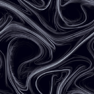
Figure 13: Snapshots of the scaled squared vorticity gradient $|\nabla\omega|^{2}$ at $t=61$ for the case $\mu=0.1$ (upper) and at $t=65$ for the case $\mu=0.2$ (lower). Light areas are regions of large values, and dark areas are regions of small values.

Filament structures can clearly be seen for both cases, showing that the measure $p_{i}$ concentrates in a very small area. This is particularly clear in the case $\mu=0.2$.

To quantify the multifractal nature of $p_{i}$, we now calculate its Rényi dimension spectrum $D_{q}$. We employ the box-counting method to estimate $D_{q}$. Using box size $\epsilon/L$ ranging from $2^{-12}$ to $2^{-1}$, we compute the instantaneous $I_{1}(q,\epsilon)$ from $t=41$ to $t=75$ at every 1 time unit using the numerical solution of Eq. (2). For $q\neq 1$, we then make log-log plot of the time-average of $[I_{1}/(q-1)]$ versus $\epsilon/L$. These are shown in FIGS. 14(a) and 15(a). For $q=1$, we take the limit $q\rightarrow 1$ in Eq. (46) to obtain $I_{2}(\epsilon)\sim\epsilon^{D_{1}}$, where

$$I_{2}(\epsilon)=\sum_{i}p_{i}(\epsilon)\log_{2}[p_{i}(\epsilon)]\ ,$$ (53)

and for $q=1$ in FIGS. 14(a) and 15(a), the time average of $I_{2}(\epsilon)$ is plotted against $\log_{2}(\epsilon/L)$. According to Eq. (46), these plots will show a linear region with slope equals $D_{q}$. All curves in FIGS. 14(a) and 15(a) show slightly undulating behavior which introduces uncertainties in the determination of $D_{q}$. The estimated $D_{q}$ at different values of $q$ are shown as circles with error bars in FIGS. 14(b) and 15(b). The error bars correspond to the variability of the $D_{q}$ observed at different moments in time.

Figure 14: For the case of $\mu=0.1$: (a) $I_{1}(q,\epsilon)$ for $q$ between 0.1 and 2.0 ($I_{2}(\epsilon)$ is plotted for $q=1.0$). The dotted lines are linear fits in the scaling region. (b) $D_{q}$ computed using numerical solution of Eq. (2) (circle with error bar) and its fourth degree polynomial fit (dotted line). $D_{q}$ predicted by the theory Eq. (51) when $\zeta_{2q}$ obtained from numerical simulations are used (square) and when $\zeta_{2q}$ calculated from Eq. (20) are used (diamond).

Figure 15: For the case of $\mu=0.2$: (a) $I_{1}(q,\epsilon)$ for $q$ between 0.1 and 2.0 ($I_{2}(\epsilon)$ is plotted for $q=1.0$). The dotted lines are linear fits in the scaling region. (b) $D_{q}$ computed using numerical solution of Eq. (2) (circle with error bar) and its fourth degree polynomial fit (dotted line). $D_{q}$ predicted by the theory Eq. (51) when $\zeta_{2q}$ obtained from numerical simulations are used (square) and when $\zeta_{2q}$ calculated from Eq. (20) are used (diamond).

The dotted lines in the figures are fourth degree polynomials fitted to the circles. We also compute $D_{q}$ using Eq. (51). To this end, we fit the curves of $\zeta_{2q}/\zeta_{2}$ versus $q$ in FIG. 7(b) and FIG. 8(b) with the following polynomial, where $d=3$ for the circles and $d=5$ for the crosses,

$$\frac{\zeta_{2q}}{\zeta_{2}}=q\left[1+\sum_{n=1}^{d}a_{n}(q-1)^{n}\right]\ .$$ (54)

By Eq. (51), $D_{q}$ is then given by

$$D_{q}=2+\zeta_{2}\sum_{n=1}^{d}a_{n}q(q-1)^{n-1}\ .$$ (55)

In FIGS. 14(b) and 15(b), we plot Eq. (55) using $\zeta_{2q}$ obtained from numerical simulations, as well as $\zeta_{2q}$ calculated from our theory. The results are shown as solid lines labeled with squares and diamonds, respectively. Despite the fact that there are discrepancies between the $D_{q}$ obtained by the various methods, they all show the same trend and clearly indicates that $p_{i}$ is multifractal (i.e., $D_{q}$ varies with $q$).

We now generate the singularity spectrum $f(\alpha)$ by Legendre transforming the $D_{q}$ curves shown in FIGS. 14(b) and 15(b). In particular, for each value of $q$, we have Halsey et al. (1986)

$$\alpha(q) = \frac{d}{dq}\left[(q-1)D_{q}\right]\ ,$$ (56)

$$f[\alpha(q)] = \alpha q-(q-1)D_{q}\ .$$ (57)

In the absence of intermittency $D_{q}$ is independent of $q$ and $f(\alpha)$ is defined only at $\alpha=D_{q}$. Thus the consistent determination of $f(\alpha)$ over some range of $\alpha$ indicates intermittency. FIG. 16 and FIG. 17 show the $f(\alpha)$ obtained for $\mu=0.1$ and $\mu=0.2$ respectively using the $D_{q}$ obtained by the three methods in FIG. 14(b) and 15(b) (circle, square and diamond symbols).

Figure 16: For the case of $\mu=0.1$: The $f(\alpha)$ curves generated by Legendre transforming the $D_{q}$ curves in FIG. 14(b) with the corresponding labels (circle, square and diamond). $f(\bar{\alpha})$ at different values of $\bar{\alpha}$ obtained by the canonical method is shown as well (cross).

Figure 17: For the case of $\mu=0.2$: The $f(\alpha)$ curves generated by Legendre transforming the $D_{q}$ curves in FIG. 15(b) with the corresponding labels (circle, square and diamond). $f(\bar{\alpha})$ at different values of $\bar{\alpha}$ obtained by the canonical method is shown as well (cross).

The results for $f(\alpha)$ are seen to agree very well with each other in spite of the difference between the $D_{q}$ determinations. Thus, we find that $f(\alpha)$ gives a more consistent measure of intermittency across different methods of determination than does $D_{q}$. We believe that the disagreement seen in FIGS. 14(b) and 15(b) between the different methods for determining $D_{q}$ is not significant in view the limited amount of scaling range available.

We can also determine $f(\alpha)$ directly from the numerical solution of Eq. (2). Following Ref. Chhabra et al. (1989), we use the canonical method developed in Ref. Chhabra and Jensen (1989) to determine $f(\alpha)$. Accordingly, we construct the normalized $q^{\mathrm{th}}$ order measures $m_{i}(q,\epsilon)$ in box $\mathcal{R}_{i}(\epsilon)$ as follow,

$$m_{i}(q,\epsilon)=\frac{p^{q}_{i}(\epsilon)}{\sum_{j}p^{q}_{j}(\epsilon)}\ .$$ (58)

Then, the mean singularity index $\bar{\alpha}$ and the corresponding $f(\bar{\alpha})$ is given by

$$\bar{\alpha}(q)=\sum_{i}m_{i}\alpha_{i} =\lim_{\epsilon\rightarrow 0}\lim_{\nu\rightarrow 0}\frac{\sum_{i}m_{i}\log p_{i}}{\log\epsilon}\ ,$$ (59)

$$f[\bar{\alpha}(q)] =\lim_{\epsilon\rightarrow 0}\lim_{\nu\rightarrow 0}\frac{\sum_{i}m_{i}\log m_{i}}{\log\epsilon}\ .$$ (60)

One of the advantages of the canonical method is the absence of finite-size effect due to logarithmic prefactors Chhabra et al. (1989). To estimate $\bar{\alpha}$, we plot the time average of the quantity $\sum_{i}m_{i}\log_{2}p_{i}$ versus $\log_{2}(\epsilon/L)$ and measure the slopes in the scaling region. Similarly, when we plot the time average of $\sum_{i}m_{i}\log_{2}m_{i}$ versus $\log_{2}(\epsilon/L)$, the slopes in the scaling range give the values of $f(\bar{\alpha})$. For the case $q=1$, $\bar{\alpha}(1)=f[\bar{\alpha}(1)]$ is obtained by measuring the slope of the curve of the time-averaged $I_{2}(1,\epsilon)$ versus $\log_{2}(\epsilon/L)$. The values of $f(\bar{\alpha})$ at different values of $\bar{\alpha}$ obtained by this scheme are shown as crosses in FIG. 16 and FIG. 17 for $\mu=0.1$ and $\mu=0.2$ respectively. They are in excellent agreement with the $f(\alpha)$ generated by Legendre transforming the $D_{q}$ curve obtained from the numerical solution of Eq. (2).

V.3 Discussion

Kolmogorov introduced the refined similarity hypothesis (RSH) Eq. (42) to take into account the spatial fluctuations of $\varepsilon$ in three-dimensional turbulence. The relation Eq. (43) is a direct consequence of the RSH. In two-dimensional turbulence, the relevant quantity is the local rate of viscous enstrophy dissipation $\eta$. We have already seen that the measure $p_{i}$ is multifractal in the presence of drag, indicating the intermittent nature of $\eta$. Following Kolmogorov’s ideas, we consider the average of $\eta$ over an area $\mathcal{R}(r)$ of linear dimension $r$:

$$\eta_{r}=\frac{\nu}{r^{2}}\int_{\mathcal{R}(r)}|\nabla\omega|^{2}\,d\vec{x}\ .$$ (61)

Analogous to the Kolmogorov’s RSH, we propose that at high Reynolds number, there is an inertial range of $r$ in which

$$\langle|\delta_{\vec{r}}\omega|^{2q}\ \vline\ \eta_{r}\rangle=C_{2q}(r^{\zeta_{2}}\eta_{r})^{q}$$ (62)

where $C_{2q}$ are constants. Eq. (62) implies $\langle|\delta_{\vec{r}}\omega|^{2q}\rangle\sim\langle(\eta_{r})^{q}\rangle r^{q\zeta_{2}}$ and hence $\langle(\eta_{r})^{q}\rangle\sim r^{\gamma_{q}}$ with

$$\gamma_{q}=\zeta_{2q}-q\zeta_{2}\ .$$ (63)

An expression analogous to Eq. (63) has been proven for Kraichnan’s model of passive scalar advection Kraichnan et al. (1995); Chertkov and Falkovich (1996). We note that Eq. (62) follows if

$$\eta_{r}\sim\frac{(\delta_{\vec{r}}\omega)^{2}}{r^{\zeta_{2}}}$$ (64)

which is the two-dimensional counterpart of Eq. (44). It is straightforward to show that the hypothesis Eq. (62) implies Eq. (51). Denoting $\eta_{r}$ in box $\mathcal{R}_{i}(r)$ by $\eta_{r}^{(i)}$, we have

$$p_{i}(r)=\frac{r^{2}}{L^{2}}\frac{\eta_{r}^{(i)}}{\langle\eta\rangle}\ .$$ (65)

Since $\sum_{i}[\eta_{r}^{(i)}]^{q}\sim r^{-2}\langle(\eta_{r})^{q}\rangle$, we get $I(q,r)\sim r^{2q-2+\gamma_{q}}$, from which Eq. (51) immediately follows.

Finally, we remark that if the measure $p_{i}$ is defined with a parameter $n$ as follow Városi et al. (1991),

$$p_{i}(\epsilon,n)=\frac{\int_{\mathcal{R}_{i}(\epsilon)}|\nabla\omega|^{n}\,d\vec{x}}{\int_{\mathcal{R}}|\nabla\omega|^{n}\,d\vec{x}}\ ,$$ (66)

then the corresponding formula for the $D_{q}$ based on this measure is

$$D_{q}=2+\frac{\zeta_{nq}-q\zeta_{n}}{q-1}\ .$$ (67)

VI Conclusion

We have studied the enstrophy cascade regime of two-dimensional turbulence with linear drag. A previous theory for the power law exponent of the energy wavenumber spectrum is verified by direct numerical computation using a $4096\times 4096$ lattice. We also calculate the vorticity structure functions numerically and show that they exhibit anomalous scaling in the presence of drag. The values of the structure function scaling exponents $\zeta_{2q}$ are measured and found to agree with the prediction by previous theory. We then compute the probability distribution function $\bar{P}_{r}(X_{\vec{r}})$ of the standardized vorticity difference $X_{\vec{r}}$ and find that $\bar{P}_{r}(X_{\vec{r}})$ develops exponential and stretched-exponential tails at small values of $r$. The theoretical expression for $\bar{P}_{r}(X_{\vec{r}})$ is shown to give predictions that agree well with the numerical results for a wide range of $r$. A measure based on the local viscous enstrophy dissipation rate $\eta$ is studied in terms of its Rényi dimension spectrum $D_{q}$ and singularity spectrum $f(\alpha)$, and is found to be multifractal. The intermittency in $\eta$ is connected to the intermittency in vorticity difference by a two-dimensional analog of the refined similarity hypothesis, and we derive a formula that relates $D_{q}$ to $\zeta_{2q}$.