Flow equations for the one-dimensional Kondo lattice model: Static and dynamic ground state properties

Abstract

The one-dimensional Kondo lattice model is investigated by means of Wegner’s flow equation method. The renormalization procedure leads to an effective Hamiltonian which describes a free one-dimensional electron gas and a Heisenberg chain. The localised spins of the effective model are coupled by the well-known RKKY interaction. They are treated within a Schwinger boson mean field theory which permits the calculation of static and dynamic correlation functions. In the regime of small interaction strength static expectation values agree well with the expected Luttinger liquid behaviour. The parameter $K_{\rho}$ of the Luttinger liquid theory is estimated and compared to recent results from density matrix renormalization group studies.

I Introduction

The fascinating subject of heavy fermion physics in rare-earth and actinide systems has been a challenge for theoretical and experimental investigations for decades fulde . The intriguing properties of these materials are far from being understood and still give us a lot of puzzles to solve. Theoretical studies of the heavy fermion materials are based on several models like the periodic Anderson model (PAM) hewson . Another generic model is the Kondo lattice model (KLM) which describes a noninteracting electron gas coupled to localised spin moments via a Heisenberg spin interaction. The Hamiltonian reads

$${\cal H}=\sum_{k\sigma}\varepsilon_{k}\;c^{\dagger}_{k\sigma}c_{k\sigma}+\frac{J}{2}\,\sum_{i\,\alpha\beta}{\bf S}_{i}\,c^{\dagger}_{i\alpha}{\boldsymbol{\sigma}}_{\alpha\beta}\,c_{i\beta},$$ (1)

where $\varepsilon_{k}=-\sum_{ij}t_{ij}\,\text{e}^{ik(R_{i}-R_{j})}$ is the dispersion relation for the electrons on the lattice, $t_{ij}$ being the hopping integrals. The parameter $J$ is the exchange integral of the local spin interaction, the so called Kondo exchange.

We want to consider here the one-dimensional case which has been the subject of numerous numerical and analytical investigations. Numerical studies were based on the Quantum Monte Carlo (QMC) method troyer_wuertz , exact diagonalization (ED) studies tsunetsugu_rmp ; tsunetsugu_prb , the density matrix renormalization group (DMRG) moukouri_caron ; caprara_rosengren ; shibata_jp ; xavier_1 ; shibata_tsunetsugu or the numerical renormalization group (NRG) method yu_white . Analytical approaches comprised the bosonisation technique honner_gulacsi ; mcculloch or the renormalization group (RG) theory pivovarov_si .

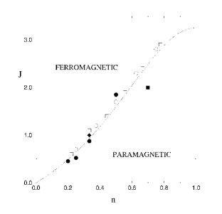
Figure 1: Phase diagram after honner_gulacsi

The phase diagram of the one-dimensional KLM as a function of the Kondo coupling $J$ and the band filling $n_{c}$ of the conduction electrons is quite accurately known. In higher dimensions the KLM is believed to show the well-known Doniach phase diagram doniach . In contrast to the latter the one-dimensional model does not exhibit a magnetically ordered phase in the parameter regime of small interaction strengths $J$. In this parameter regime the corresponding phase diagram is governed by a paramagnetic metallic phase tsunetsugu_rmp . There, the model is assumed to belong to the universality class of the so called Luttinger liquids luttinger which possess gapless charge and spin excitations resulting in an algebraic decay of the corresponding correlation functions. The asymptotic form for density-density- and spin-spin-correlations are voit

$$\left<\delta n(x)\delta n(0)\right>=\frac{K_{\rho}}{(\pi\,x)^{2}} +A_{1}\cos(2k_{F}x)\,x^{-1-K_{\rho}}\allowdisplaybreaks$$

$$+A_{2}\cos(4k_{F}x)\,x^{-4K_{\rho}}\allowdisplaybreaks$$ (2)

$$\left<{\bf S}(x)\cdot{\bf S}(0)\right>=\frac{1}{(\pi\,x)^{2}} +B_{1}\cos(2k_{F}x)\,x^{-1-K_{\rho}}.$$ (3)

The parameter $K_{\rho}$ is a model dependent constant which determines the low-energy physics. Apart from the paramagnetic metallic phase for small $J/t$ the phase diagram further comprises a ferromagnetic ordered phase for large $J$ and a spin liquid insulator phase at half-filling, $n_{c}=1$. There are two limiting cases in which the ground state has been proven to be ferromagnetic tsunetsugu_rmp . Firstly, the limit of vanishing electron density $n_{c}\to 0$, secondly the case of infinite coupling strength $J/t\to\infty$. The situation at half filling is special in the sense that it exhibits finite gaps for spin and charge excitations at any finite coupling $J$.

The KLM can be understood as an effective Hamiltonian of the above mentioned PAM. It is connected to the PAM by a Schrieffer-Wolff transformation schrieffer_wolff . This property naturally raises the question whether the localised spins in the KLM participate in the formation of the Fermi surface, or in other words: Does $k_{F}=n_{c}\pi/2$ or $k_{F}=(n_{c}+1)\pi/2$ hold? The size of the Fermi surface can be read from the positions of singularities in certain correlation functions. Recent results seemed to confirm the picture of a small Fermi surface with $k_{F}=n_{c}\pi/2$ xavier_1 . However, a more careful analysis which has recently been performed by Shibata et al. shibata_new supports a large Fermi surface.

In this paper we shall apply the analytical method of continuous unitary transformations (flow equations) proposed by Wegner wegner and Głazek/Wilson glazek_wilson to the one-dimensional KLM. It was first applied to this model in arbitrary dimensions by Stein stein . He derived an analytical expression for the RKKY interaction.

In Sec. II we shall give a short introduction into the flow equation method. In Sec. III the method will be applied to the one-dimensional KLM. By integrating out the Kondo coupling between the conduction electrons and localised spins we arrive at a decoupled system of a renormalized noninteracting one-dimensional electron gas and a renormalized spin chain. In the latter the spins interact via an effective spin exchange. Within the framework of the flow equation method it is straightforward to find expectation values and correlation functions, if the eigenvalue problem of the effective model is known. In Sec. IV we shall show how the method can be used in order to verify the expected characteristic behaviour of a Luttinger liquid. Previous investigations of the one-dimensional KLM have mainly focused on static properties like the momentum distribution or spin and charge correlation functions. In this work we shall put special emphasis on the investigation of dynamic properties and extend already existing results for the dynamics.

II Flow equation method

To begin with we would like to sketch the concept of the flow equation method which was independently developed by Wegner wegner and Głazek/Wilson glazek_wilson in 1994. Since then the method has successfully been applied to a great number of problems, e.g. the electron-phonon-problem electron_phonon , one-dimensional interacting fermion systems 1d_systeme or the spin-boson-problem spin_boson .

The basic idea of the flow equation method is the application of a continuous set of unitary transformations to a given Hamiltonian

$${\cal H}(l)={\cal U}(l)\,{\cal H}\,{\cal U}^{\dagger}(l).$$ (4)

Here $l$ means the continuous flow parameter. The purpose of this procedure is that one wishes to diagonalize or at least simplify the Hamiltonian. Thereby the parameters of the Hamiltonian become renormalized. This treatment is translated into the language of differential equations by using the expression

$$\eta(l)=\frac{d\,{\cal U}(l)}{dl}\,{\cal U}^{\dagger}(l)$$ (5)

for the antihermitean generator $\eta(l)=-\eta^{\dagger}(l)$ of the unitary transformation. The differential equation for the Hamiltonian takes the simple form

$$\frac{d\,{\cal H}(l)}{dl}=\left[\eta(l),{\cal H}(l)\right].$$ (6)

The generator has to be suitably chosen. Wegner’s approach starts from a decomposition of the Hamiltonian into an unperturbed part ${\cal H}_{0}$, whose eigenvalue problem is assumed to be known, and a perturbation ${\cal H}_{1}$. Wegner’s generator is given by

$$\eta(l)=\left[{\cal H}_{0}(l),{\cal H}(l)\right]$$ (7)

which is simply the commutator between the unperturbed part ${\cal H}_{0}(l)$ and the perturbation ${\cal H}_{1}(l)$. This generator integrates out all interaction terms except for possible degenerations wegner . It finally leads to a diagonal or block-diagonal effective Hamiltonian.

III Flow equations for the Kondo lattice model

We now turn to the derivation of the flow equations for the parameters of the Hamiltonian. With this in mind we proceed as follows. Firstly, we give the flow invariant Hamiltonian which includes new generated, effective interactions. The flow invariant Hamiltonian then leads us to the specification of the generator. Thereby we shall introduce some of the necessary approximations within our approach.

III.1 Flow equations for the Hamiltonian

The first step in deriving the flow equations is the determination of the generator $\eta(l)$. In a first step we wish to integrate out the Kondo coupling between the conduction electrons and the localised spins, so the most simple generator is

$$\eta(l)=\frac{1}{2N}\,\sum_{ikq\,\alpha\beta}\eta^{J}_{kq}(l)\,{\bf S}_{i}\cdot{\boldsymbol{\sigma}}_{\alpha\beta}\,c^{\dagger}_{k\alpha}c_{q\beta}\;\text{e}^{i(k-q)R_{i}}=:\eta^{J}(l),$$ (8)

where the coefficients $\eta^{J}_{kq}(l)$ are still unspecified. They depend on the concrete choice of the generator. Wegner’s approach starts out from the generalised form of Eq. (7). If we take only the conduction electrons to be ${\cal H}_{0}$, we obtain $\eta_{kq}(l)=(\varepsilon_{k}-\varepsilon_{q})J_{kq}(l)$ for the coefficients of the generator. The commutator between the generator (8) and the Hamiltonian (1) gives rise to new, effective interactions. Using Wegner’s approach they enter the generator and are eventually integrated out. We shall introduce a more general form of $\eta(l)$ below.

In order to see what kind of effective interactions emerge, let us commute the initial Hamiltonian (1) and the generator of Eq. (8). After some calculation we obtain the following Hamiltonian

$${\cal H}(l) =\sum_{k\sigma}\varepsilon_{k}(l):c^{\dagger}_{k\sigma}c_{k\sigma}:+\frac{1}{2N}\,\sum_{kq}\chi_{kq}(l)\,:{\bf S}_{k-q}\cdot{\bf S}_{q-k}:+E_{c}(l)\allowdisplaybreaks$$

$$+\frac{1}{2N}\,\sum_{kq\,\alpha\beta}J_{kq}(l)\,{\bf S}_{k-q}\cdot{\boldsymbol{\sigma}}_{\alpha\beta}\,:c^{\dagger}_{k\alpha}c_{q\beta}:+\frac{1}{4N^{2}}\sum_{kpq\sigma}M_{kpq}(l):{\bf S}_{k-p}\cdot{\bf S}_{p-q}:\,:c^{\dagger}_{k\sigma}c_{q\sigma}:\allowdisplaybreaks$$

$$+\frac{1}{4N^{2}}\sum_{kpq\alpha\beta}iD_{kpq}(l)\,({\bf S}_{k-p}\times{\bf S}_{p-q})\cdot{\boldsymbol{\sigma}}_{\alpha\beta}:c^{\dagger}_{k\alpha}c_{q\beta}:\allowdisplaybreaks$$

$$={\cal H}_{e}(l)+{\cal H}_{S}(l)+E_{c}(l)+{\cal H}_{J}(l)+{\cal H}_{M}(l)+{\cal H}_{D}(l),$$ (9)

where $:{\cal X}:$ denote operators resulting from a decoupling scheme which we shall discuss later.

Before we proceed let us take a closer look at equation (9). The first line represents the block diagonal part of the Hamiltonian since electron and spin operators are decoupled. It contains a complicated RKKY-like spin interaction term between the local moments. The second and third line comprise the nondiagonal or interaction part. Aside from the Kondo coupling we get interactions between the local moments which are either symmetric or antisymmetric with respect to interchange of the sites. Correspondingly, the first one couples to the electronic charge density, whereas the second one couples to the electronic spin density. We restrict ourselves to these terms because they are the most important ones in the regime of small interaction strength $J$. That way the above Hamiltonian becomes flow invariant and Eq. (9) is valid for all flow parameters $l$. For $l=0$ it represents the initial Hamiltonian (1). This implies the following initial values of the parameters

$$\varepsilon_{k}(l=0) =\varepsilon_{k}\,,\qquad J_{kq}(l=0)=J\allowdisplaybreaks$$

$$\chi_{kq}(l=0) =0\,,\qquad M_{kpq}(l=0)=0\allowdisplaybreaks$$

$$D_{kpq}(l=0) =0\,,\qquad E_{c}(l=0)=\sum_{k}\varepsilon_{k}n_{k}.$$ (10)

The prefactor of any operator term of Eq. (9) controls the strength of the respective operator. Within the framework of the flow equation method they are determined by corresponding differential equations. With the choice of the generator $\eta(l)$ we can control which of these terms are kept and which are to be vanished. Since the aim of our renormalization procedure is a blockdiagonal Hamiltonian in which electron and spin operators are decoupled, we have to remove all terms describing interactions between electron and spin operators. The generator $\eta(l)$ of the continuous unitary transformation has to be chosen appropriately.

With this in mind we can now write down the generator $\eta(l)$. Using Wegner’s approach we have to take into account the generated, effective interactions. The generator reads

$$\eta(l)=\eta^{J}(l)+\eta^{M}(l)+\eta^{D}(l) =\frac{1}{2N}\sum_{kq\alpha\beta}\eta^{J}_{kq}(l)\;{\bf S}_{k-q}\cdot{\boldsymbol{\sigma}}_{\alpha\beta}\,:c^{\dagger}_{k\alpha}c_{q\beta}:+\frac{1}{4N^{2}}\sum_{kpq\sigma}\eta^{M}_{kpq}(l):{\bf S}_{k-p}\cdot{\bf S}_{p-q}:\,:c^{\dagger}_{k\sigma}c_{q\sigma}:$$

$$+\frac{1}{4N^{2}}\sum_{kpq\alpha\beta}\eta^{D}_{kpq}(l)\;i({\bf S}_{k-p}\times{\bf S}_{p-q})\cdot{\boldsymbol{\sigma}}_{\alpha\beta}\,:c^{\dagger}_{k\alpha}c_{q\beta}:$$ (11)

and the prefactors $\eta^{J}_{kq}(l)$, $\eta^{D}_{kpq}(l)$ and $\eta^{M}_{kpq}(l)$ are determined by Eq. (7).

After the transformation, i.e. in the limit $l\to\infty$, only the first line of Eq. (9) remains. It represents the diagonal part ${\cal H}_{0}(l)$. This effective Hamiltonian can be used to easily calculate physical properties. The nondiagonal part ${\cal H}_{1}(l)$ vanishes for $l\to\infty$ and the effective Hamiltonian $\tilde{\cal H}:={\cal H}(l=\infty)$ then reads

$$\tilde{\cal H} =\sum_{k\sigma}\tilde{\varepsilon}_{k}:c^{\dagger}_{k\sigma}c_{k\sigma}:+\frac{1}{2N}\,\sum_{kq}\tilde{\chi}_{kq}\,:{\bf S}_{k-q}\cdot{\bf S}_{q-k}:+\tilde{E}_{c}$$

$$=\tilde{\cal H}_{e}+\tilde{\cal H}_{S}+\tilde{E}_{c}.$$ (12)

In the following we shall denote all renormalized variables by a tilde. As Eq. (12) tells us the effective model will consist of a one-dimensional noninteracting electron gas and a Heisenberg spin chain with renormalized parameters.

We now have all ingredients needed to derive the flow equations for the parameters of the Hamiltonian. Before doing this we want to look at the approximations that have to be done. Firstly, we neglect interactions of order ${\cal O}(J^{3})$ and higher in the Hamiltonian (9). Secondly, we decouple higher operator products in order to reduce them to those appearing in ${\cal H}(l)$. This gives rise to operator expressions of the form $:{\cal X}:$. They refer to fluctuation operators and mean either a normal order product of fermionic operators or a Hartree-Fock-decoupling scheme of spin operator products

$$:c^{\dagger}_{k\sigma}c_{k\sigma}: =c^{\dagger}_{k\sigma}c_{k\sigma}-\langle c^{\dagger}_{k\sigma}c_{k\sigma}\rangle,\allowdisplaybreaks$$ (13)

$$:{\bf S}_{k-q}\cdot{\bf S}_{q-k}: ={\bf S}_{k-q}\cdot{\bf S}_{q-k}-\langle{\bf S}_{k-q}\cdot{\bf S}_{q-k}\rangle.$$ (14)

The thermodynamic average will here be taken with respect to the effective model $\tilde{\cal H}$, Eq. (12), which describes a decoupled system of a simple Fermi gas (electrons) and a Heisenberg spin chain with long-range interactions. These expectation values are therefore $l$-independent. The decoupling leads to a formal temperature dependence of the flow equations. Here we consider only the ground state properties, i.e. $T=0$. For the sake of simplicity we introduce the abbreviation $S(k-q):=\langle{\bf S}_{k-q}\cdot{\bf S}_{q-k}\rangle$ for the spin correlation function. One may also think of other expectation values like $\langle{\bf S}_{k-q}\times{\bf S}_{q-k}\rangle$ or $\langle{\bf S}_{q}\rangle$. Since we consider the limit of small Kondo coupling $J$, the system is in the paramagnetic phase, where no symmetry is broken. Therefore these expectation values vanish.

Evaluating the commutator between the generator (11) and the Hamiltonian (9) we arrive at the flow equations for the parameters of the Hamiltonian. For the sake of clarity the $l$-dependence of all parameters is dropped. The electronic single particle energies $\varepsilon_{k}$ obey the following differential equation

$$\frac{d\varepsilon_{k}}{dl}=\frac{1}{2N}\sum_{q}S(k-q)\,\eta^{J}_{kq}\,J_{qk}.$$ (15)

Here $S(k-q)$ is the local moment’s spin correlation function which has to be evaluated with respect to the renormalized Hamiltonian $\tilde{\cal H}$. It is therefore $l$-independent. As the effective model is not known before the end of the transformation we have to solve all flow equations self-consistently.

For the paramter $\chi_{kq}$ of the effective spin interaction we obtain the following flow equation

$$\frac{d\chi_{kq}}{dl} =(n_{k}-n_{q})\,\eta^{J}_{kq}\,J_{qk}.$$ (16)

The occupation numbers $n_{k}$ which enter the above equation are again formed with respect to the effective model. The constant $E_{c}$ of ${\cal H}_{0}(l)$ follows

$$\frac{dE_{c}}{dl} =\frac{1}{N}\sum_{kq}(n_{k}-n_{q})\,S(k-q)\,\eta^{J}_{kq}\,J_{qk}.$$ (17)

We restrict the renormalization of the effective interaction terms to contributions of order ${\cal O}(J^{2})$. Therefore both coupling parameters $D_{kpq}$ and $M_{kpq}$ obey the same flow equation

$$\frac{dD_{kpq}}{dl} =\frac{1}{2}(\eta^{J}_{kp}J_{pq}+\eta^{J}_{qp}J_{kp})-(\varepsilon_{k}-\varepsilon_{q})\,\eta^{D}_{kpq}.$$ (18)

The first term is responsible for the generation of the effective coupling while the second contribution, which is always negative, ensures the vanishing at the end of the renormalization procedure. Finally for the flow equation of the Kondo coupling we find

$$\frac{dJ_{kq}}{dl} =-(\varepsilon_{k}-\varepsilon_{q})\eta^{J}_{kq}\allowdisplaybreaks$$

$$+\frac{1}{N}\sum_{p}\left(n_{p}-\frac{1}{2}\right)(\eta^{J}_{kp}J_{pq}+\eta^{J}_{qp}J_{pk})\allowdisplaybreaks$$

$$+\frac{3}{8N}\sum_{p}(\eta^{J}_{kp}D_{pkq}+\eta^{J}_{qp}D_{pqk})\allowdisplaybreaks$$

$$+\frac{3}{8N}\sum_{p}(\eta^{D}_{kqp}J_{pk}+\eta^{D}_{qkp}J_{pk})\allowdisplaybreaks$$

$$-\frac{1}{8N}\sum_{p}(\eta^{J}_{kp}D_{p,p+q-k,q}+\eta^{J}_{qp}D_{p,p+k-q,k})\allowdisplaybreaks$$

$$-\frac{1}{8N}\sum_{p}(\eta^{D}_{k,p+q-k,p}J_{pk}+\eta^{D}_{q,p+k-q,p}J_{pk}),$$ (19)

where we have taken into account correction terms up to order ${\cal O}(J^{3})$. Therefore we expect to find reasonable results only in the parameter regime of small coupling strength $J/t$. As this ratio increases further correction terms have to be included. The flow equations (15) to (19) represent a closed system of first order differential equations, whose solution can only be found by numerical integration.

III.2 Approximations for the effective model

In the preceeding subsection we have derived flow equations for the parameters of the Hamiltonian. As to solve them we still need an analytical expression for the spin correlation function $S(k-q)$. As it describes spin correlations of the effective model, we are dealing here with a one-dimensional Heisenberg chain with long-range interactions whose exact solution is not known. Hence, we have to resort to further approximations. We stress here that this is the most crucial approximation within our approach because it strongly affects all renormalized quantities. Since the spin interaction is the result of the continuous unitary transformation it is not known until the transformation is completely performed.
As our approach is only valid for small $J/t$, i.e. for the paramagnetic metallic phase with no broken symmetry, we use the Schwinger boson formalism to describe the spin system arovas_auerbach . It preserves the rotational invariance of the spin Hamiltonian. The spin operators are expressed in terms of Schwinger bosons $a_{i\sigma}$ and $a^{\dagger}_{i\sigma}$ according to

$$S^{\gamma}_{i}=\frac{1}{2}\;\sum_{\sigma\sigma^{\prime}}a^{\dagger}_{i\sigma}\,\sigma^{\gamma}_{\sigma\sigma^{\prime}}a_{i\sigma^{\prime}},$$ (20)

where $\sigma^{\gamma}_{\sigma\sigma^{\prime}}$ stands for the Pauli spin matrix. Since the occupation number for bosons is not restricted, a local constrained of the form $\sum_{\sigma}\;a^{\dagger}_{i\sigma}a_{i\sigma}=2S$ must be enforced.

We follow here the procedure of Trumper et al. trumper_manuel_gazza_ceccatto or of Ceccatto et al. ceccatto_gazza_trumper and introduce two fields

$$A_{ij} =\frac{1}{2}\;\sum_{\sigma}\sigma\,a_{i\sigma}a_{j\bar{\sigma}}=-A_{ji}$$ (21)

and

$$B_{ij} =\frac{1}{2}\;\sum_{\sigma}a^{\dagger}_{i\sigma}a_{j\sigma}=B^{\dagger}_{ji}$$ (22)

describing antiferro- and ferromagnetic correlations, respectively ($\bar{\sigma}=-\sigma$). This yields to the following Hamiltonian

$$\tilde{\cal H}_{S}=\sum_{ij}\;J_{ij}\,{\cal N}(B^{\dagger}_{ij}B_{ij})-A^{\dagger}_{ij}A_{ij}.$$ (23)

The expression ${\cal N}({\cal O})$ stands for a normal order product of boson operators. The Hamiltonian is now biquadratic with respect to the Schwinger boson operators. We use a mean field theory in order to decouple the biquadratic terms. By using the mean field parameters $\langle B_{ij}\rangle$ and $\langle A_{ij}\rangle$ and replacing the local constrained by a global one we obtain a Hamiltonian which can easily be diagonalized via a Bogolubov transformation. Introducing new boson operators $\alpha_{k\sigma}=u_{k}\,a_{k\sigma}+i\sigma v_{k}\,a^{\dagger}_{-k\bar{\sigma}}$ we obtain

$$\tilde{\cal H}_{S}=\sum_{q\sigma}\,\omega_{q}\,\alpha^{\dagger}_{q\sigma}\alpha_{q\sigma}+\frac{1}{2}\sum_{q\sigma}\omega_{q},$$ (24)

with $\omega(q)=\sqrt{(\gamma_{B}(q)-\lambda)^{2}-\gamma^{2}_{A}(q)}$ representing the energies of the elementary excitations $\alpha^{\dagger}_{q\sigma}$ of the spin system. Here the quantities $\gamma_{A}(q)=\frac{i}{2}\,\sum_{R_{ij}}J_{ij}\langle A_{ij}\rangle\,\text{e}^{iqR_{ij}}$ and $\gamma_{B}(q)=\frac{1}{2}\sum_{R_{ij}}J_{ij}\langle B_{ij}\rangle\,\text{e}^{iqR_{ij}}$ are used. The mean field parameters $\langle B_{ij}\rangle$ and $\langle A_{ij}\rangle$ and the Lagrange parameter $\lambda$ have to be determined selfconsistently by solving the corresponding saddle point equations.

Finally we find an analytic expression for the spin correlation function which for $T=0$ reads

$$S(q)_{T=0}=\frac{1}{4N}\sum_{k}\left(\cosh\left[2(\theta_{k}-\theta_{k+q})\right]-1\right),$$ (25)

with $\theta_{k}=-\frac{1}{2}\tanh^{-1}\left(\frac{\gamma_{A}(k)}{\gamma_{B}(k)-\lambda}\right)$.

Compared to methods like the Bethe ansatz for the nearest-neighbour Heisenberg chain the approximative Schwinger boson treatment discussed above has the advantage that as many interaction terms as possible can be taken into account. With the approximation for the effective model we are able to describe the one-dimensional KLM consistently within the framework of the flow equation method. Any physical quantity we are interested in can be evaluated within the present approach. Especially, we emphasise that nothing has to be put in by hand.

III.3 Expectation values and correlation functions

We now turn to the calculation of expectation values and correlation functions. In this subsection we give the essentials for the derivation of certain important expectation values and correlation functions. We shall discuss the results in Sec. IV.

The retarded Green’s function between operators $A$ and $B$ is in general defined as the following commutator or anticommutator relation

$$G_{AB}(t)=-i\theta(t)\langle\langle A(t);B\rangle\rangle=-i\theta(t)\langle[A(t),B]_{\pm}\rangle,$$ (26)

depending on the statistics under consideration. The thermodynamic average and the time-dependence have to be taken with respect to the full Hamiltonian. One can exploit the invariance of the trace under unitary transformations and obtains

$$G_{AB}(t)=-i\theta(t)\langle\langle\tilde{A}(t);\tilde{B}\rangle\rangle_{\tilde{\cal H}}.$$ (27)

Now the thermodynamic average and the time-dependence are taken with respect to the effective model. According to the transformation of the Hamiltonian we also have to transform the operators. They obey a similar flow equation as the Hamiltonian

$$\frac{dA(l)}{dl}=\left[\eta(l),A(l)\right].$$ (28)

The commutation between $\eta(l)$ of Eq. (11) and the electron operator $c_{k\sigma}$ leads to the following operator structure

$$c_{k\sigma}(l)=\alpha_{k}(l)\,c_{k\sigma} +\frac{1}{N}\sum_{q}\sigma\,\gamma_{kq}(l)\,S^{z}_{k-q}c_{q\sigma}$$

$$+\frac{1}{N}\sum_{q}\gamma_{kq}(l)\,S^{-\sigma}_{k-q}c_{q\bar{\sigma}},$$ (29)

where we have taken only the correction terms into account that couple to one local moment. The initial conditions of the parameters are $\alpha_{k}(l=0)=1$ and $\gamma_{kq}(l=0)=0$. We transform the spin operator according to

$$S^{z}_{i}(l)=\beta(l)S^{z}_{i} +\frac{1}{N}\sum_{kq\sigma}\,\zeta_{kq}(l)\;\sigma S^{\sigma}_{i}\text{e}^{i(k-q)R_{i}}\,c^{\dagger}_{k\bar{\sigma}}c_{q\sigma}$$ (30)

$$S^{\sigma}_{i}(l)=\beta(l)S^{\sigma}_{i} +\frac{1}{N}\sum_{kq\sigma^{\prime}}\,\zeta_{kq}(l)\;\sigma S^{\sigma}_{i}\,\text{e}^{i(k-q)R_{i}}\,\sigma^{\prime}\,c^{\dagger}_{k\sigma^{\prime}}c_{q\sigma^{\prime}}$$

$$+\frac{2}{N}\sum_{kq}\zeta_{kq}(l)\;\sigma\,S^{z}_{i}\,\text{e}^{i(k-q)R_{i}}\,c^{\dagger}_{k\sigma}c_{q\bar{\sigma}}.$$ (31)

Here the initial parameters are $\beta(l=0)=1$ and $\zeta_{kq}(l=0)=0$.

In order to derive the flow equations for the parameters of the operator transformations we have to use an equivalent decoupling scheme as for the Hamiltonian. We finally arrive at the following differential equations

$$\frac{d\alpha_{k}}{dl} =\frac{1}{2N}\sum_{q}S(k-q)\,\eta^{J}_{kq}\gamma_{qk}$$ (32)

$$\frac{d\gamma_{kq}}{dl} =\frac{1}{2}\,\eta^{J}_{qk}\,\alpha_{k}$$ (33)

for the parameters of the electron operator transformation and

$$\frac{d\beta}{dl} =-\frac{2}{N^{2}}\,\sum_{kq}\eta^{J}_{kq}\,\zeta_{kq}\,n_{k}(1-n_{q})$$ (34)

$$\frac{d\zeta_{kq}}{dl} =\frac{1}{2}\,\beta\,\eta^{J}_{qk}$$ (35)

for the parameters of the spin operator transformations. We notice that the spin correlation function $S(k-q)$ of the effective model enters the flow equation of $\alpha_{k}(l)$ whereas the occupation numbers $n_{k}$ govern the flow equation of $\beta(l)$. We restrict the flow equations for the correction terms to first order contributions in the Kondo coupling. Going beyond this approximation could bring us up against the violation of certain summation rules which have to be fullfilled. We can combine the above equations to obtain flow invariant expressions. The expectation values $S(k-q)$ and $n_{k}$ are taken with respect to the effective Hamiltonian and are therefore $l$-independent. We arrive at

$$\alpha^{2}_{k}(l)+\frac{1}{N}\sum_{q}S(k-q)\gamma^{2}_{kq}(l)=1$$ (36)

and

$$\beta^{2}(l)+\frac{4}{N^{2}}\sum_{kq}\zeta^{2}_{kq}(l)\,n_{k}(1-n_{q})=1,$$ (37)

which displays the unitarity of the transformation.

After determining the operator transformation we are now able to calculate static and dynamic correlation functions that characterise the ground state properties of the one-dimensional KLM. One of the most important quantities is the momentum distribution $n(k)$ which reads

$$n(k)=\langle c^{\dagger}_{k\sigma}c_{k\sigma}\rangle=\tilde{\alpha}^{2}_{k}\,n_{k}+\frac{1}{N}\sum_{q}\,\tilde{\gamma}^{2}_{kq}\,S(k-q)\,n_{q}.$$ (38)

For a Luttinger liquid we expect a continuous behaviour with respect to the momentum $k$ and a power law singularity at the Fermi momentum. The position of this singularity fixes the size of the Fermi surface.

The static correlation function of the local moments $S_{ff}(q)$ indicates the phase transition from the paramagnetic phase into the ferromagnetic phase on increasing the Kondo coupling $J$. Within our approach it is given by

$$S_{ff}(q) =\langle{\bf S}_{q}\cdot{\bf S}_{-q}\rangle$$

$$=\tilde{\beta}^{2}\,S(q)+\frac{4}{N^{2}}\,\sum_{kp}\tilde{\zeta}^{2}_{kp}\,S(k-p+q)\,n_{k}(1-n_{p}).$$ (39)

We can also evaluate the static charge correlation function $C(q)$ and the static spin correlation function $S_{cc}(q)$ of the electrons. Their rather lengthy expressions are given in the appendix.

The flow equation formalism allows us to calculate dynamic quantities. The first quantities we look at are the one-particle spectral functions $A_{\pm}(k,\omega)$ of the conduction electrons which measure occupied and empty states of the conduction electrons.

$$A_{+}(k,\omega) =\int_{-\infty}^{\infty}dt\langle c_{k\sigma}(t)\,c^{\dagger}_{k\sigma}\rangle\,\text{e}^{i\omega t}$$

$$=\tilde{\alpha}^{2}_{k}\,(1-n_{k})\,\delta(\omega-\tilde{\varepsilon}_{k})$$

$$+\frac{1}{2N^{2}}\,\sum_{qp}\,\tilde{\gamma}^{2}_{kq}\,(u_{p}\,v_{k+p-q}-v_{p}\,u_{k+p-q})^{2}$$

$$\hskip 49.79231pt\times(1-n_{q})\,\delta(\omega-\tilde{\varepsilon}_{q}-\tilde{\omega}_{p}-\tilde{\omega}_{k+p-q})\allowdisplaybreaks$$ (40)

$$A_{-}(k,\omega) =\int_{-\infty}^{\infty}dt\langle c^{\dagger}_{k\sigma}(t)\,c_{k\sigma}\rangle\,\text{e}^{i\omega t}$$

$$=\tilde{\alpha}^{2}_{k}\,n_{k}\,\delta(\omega-\tilde{\varepsilon}_{k})$$

$$+\frac{1}{2N^{2}}\,\sum_{qp}\,\tilde{\gamma}^{2}_{kq}\,(u_{p}\,v_{k+p-q}-v_{p}\,u_{k+p-q})^{2}$$

$$\hskip 71.13188pt\times n_{q}\,\delta(\omega-\tilde{\varepsilon}_{q}+\tilde{\omega}_{p}+\tilde{\omega}_{k+p-q}).$$ (41)

Here $u_{k}$ and $v_{k}$ are the coefficients of the Bogolubov transformation used to diagonalize the Schwinger boson mean field Hamiltonian (24). The spectral functions $A_{\pm}(k,\omega)$ comprise two contributions. The first term ($\sim\tilde{\alpha}^{2}$) represents a coherent quasiparticle excitation. The second term is an incoherent background. It is important to note that the elementary excitations of the spin system of the effective Hamiltonian $\tilde{\omega}_{q}$ enter the latter contribution. The electronic density of states defined by

$$\rho(\omega)=-\frac{1}{N}\sum_{k}\;\frac{1}{\pi}\;\text{Im}\,G(k,\omega),$$ (42)

with $G(k,\omega)$ being the electronic Green’s function, can also be calculated.

Another important quantity is the dynamic spin structure factor $S_{ff}(q,\omega)$ of the local moments

$$S_{ff}(q,\omega)=\int_{-\infty}^{\infty}dt\,\langle{\bf S}_{q}(t)\cdot{\bf S}_{-q}\rangle\,\text{e}^{i\omega t} =\frac{1}{2N}\,\sum_{p}\,\tilde{\beta}^{2}\,(u_{p}\,v_{p+q}-v_{p}\,u_{p+q})^{2}\,\delta(\omega-\tilde{\omega}_{p}-\tilde{\omega}_{p+q})\allowdisplaybreaks$$

$$+\frac{2}{N^{3}}\sum_{kpp^{\prime}}\tilde{\zeta}^{2}_{kp}(u_{p^{\prime}}v_{p^{\prime}+k-p+q}-v_{p^{\prime}}u_{p^{\prime}+k-p+q})^{2}\,n_{k}\,(1-n_{p})$$

$$\hskip 113.81102pt\times\delta(\omega-\tilde{\omega}_{p^{\prime}}-\tilde{\omega}_{p^{\prime}+k-p+q}+\tilde{\varepsilon}_{k}-\tilde{\varepsilon}_{p}).$$ (43)

The first line describes only the spin excitations of the effective model in terms of Schwinger bosons. The second line of Eq. (43) results from the coupling of the local moments to electronic particle-hole excitations of the effective Hamiltonian. In addition, we can also calculate the dynamic spin structur factor of the conduction electrons $S_{cc}(q,\omega)$ which is found in the appendix.

IV Results

After having derived theoretical expressions for various correlation functions from the flow equation approach we now turn to present the outcome of the numerical solution of the flow equations (15) - (19) and (32) - (35) . We start with the result for the parameters of the Hamiltonian and subsequently show our findings for static and dynamic correlation functions. We shall show to what extend the statics reflects the expected Luttinger liquid behaviour. We also clarify the possibility of the approach to describe the quantum phase transition on increasing coupling strength.

IV.1 Parameters of the Hamiltonian

In order to solve Eqs. (15) - (19) we used a Runge Kutta algorithm. The complexity of the differential equation restricted our system size to $N=120$. Remember that the spin correlation function $S(k-q)$ which enters the flow equations has to be calculated with respect to the effective model (12). Therefore the parameters of the Hamiltonian had to be determined self-consistently.

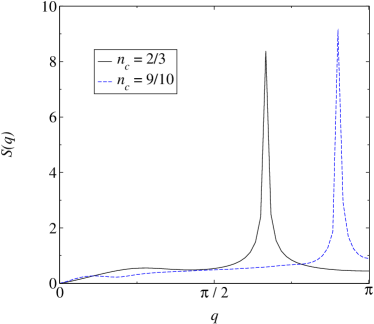
Figure 2: Spin correlation function $S(q)$ of the effective model for two different fillings $n_{c}$.

The spin correlation function $S(q)$ of the effective model plays an important role. We therefore start our discussion with $S(q)$ which is shown in Fig. 2. The main feature is the dominant peak that shows up exactly at the wave vector $q=2k_{F}^{c}=n_{c}\pi$, where $k_{F}^{c}$ is the Fermi momentum of the conduction electrons. As we shall see later the pronounced structure has severe consequences for other quantities that are related to $S(q)$. The pronounced peak is due to the special excitation spectrum of the Schwinger bosons. The other main property of $S(q)$ is the vanishing ferromagnetic component ($q=0$) which can easily be understood from Eq. (25).

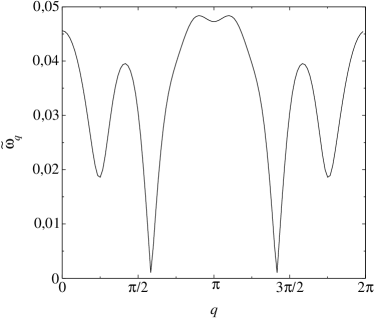
Figure 3: Elementary excitations $\tilde{\omega}_{q}$ at $n_{c}=2/3$ and $J/t=1.5$.

The elementary excitations $\tilde{\omega}_{q}$ of the spin system of $\tilde{\cal H}$ are shown in Fig. 3. They exhibit a small but finite gap at $q=k_{F}^{c}\mod\pi$. This small gap is responsible for the strong peak in $S(q)$. It manifests the rotational invariance of the ground states and is an artifact of the Schwinger boson approach as we are dealing here with half integer spins ($S=1/2$) which may have a gapless excitation spectrum. Nevertheless, within the Schwinger boson approach a vanishing gap would give rise to a ground state with broken symmetry that contradicts the assumption of a rotational invariant paramagnetic phase. However, the important point is the position of this gap. It determines the maximum of the spin correlation function which turns out to be at the expected position. Therefore we assume that a description in terms of spinons should not change these results decisively. Looking at Eq. (25) we see that always pairs of excitations enter the equation for $S(q)$ so that the maximum of the spin correlation function is found at $q=2k_{F}^{c}=n_{c}\pi$.

At this point we add that we found solutions for the saddle point equations of the SBMFT only in the parameter regime $1/2<n_{c}<1$. The case of half filling is special in the sense that there exists a gapped spin liquid phase. It remains an open question whether the present approach can also be used to describe this phase. Below $n_{c}=1/2$ the dominance of the ferromagnetic components in the RKKY coupling ${\cal J}_{ij}$ prevents a solution of the saddle point equations of the SBMFT.

Figure 4: Renormalized electronic single particle energies $\tilde{\varepsilon}_{k}$ at $n_{c}=2/3$ and different values $J/t$.

Finally we discuss the renormalized electronic single-particle energies. The dispersion relation $\tilde{\varepsilon}_{k}$ is presented in Fig. 4. We assume the unrenormalized single-particle energies to follow a tight binding dispersion $\varepsilon_{k}=-2t(\cos k-1)$, where we set the bottom of the band equal to zero and $t=1/2$. We recognise two basic features for $\tilde{\varepsilon}_{k}$. The first is a broadening of the band. The effective band width is enlarged compared with the original band width $W=4t$. The other one is a decreasing density of states at the Fermi momentum $k=k_{F}^{c}$ and at $k=\pi-k_{F}^{c}$. This property is mainly due to the dominant peak structure in the spin correlation function $S(q)$ at $q=2k_{F}^{c}$. The wave vector $q=2k_{F}^{c}$ connects the two points of the Fermi surface. Therefore the energies near the Fermi surface become more strongly renormalized than energies near the band edge. The pseudo-gap like structure at $k=k_{F}^{c}$ is thus due to the strong spin fluctuations at $q=2k_{F}^{c}$. As we are going to see this behaviour shall have consequences for the electronic density of states $\rho(\omega)$. As the Luttinger liquid theory expects $\rho(\omega)$ to vanish at $\omega=0$ a decreasing density of states in the renormalized electron spectrum is reasonable. In order to resolve the observed structures in the renormalized electron spectrum we need to examine larger systems.

IV.2 Static properties

Let us now study the static correlation functions calculated in the last section. The first quantity we want to consider is the momentum distribution function $n(k)$ which is shown in Fig. 5. We obtain meaningful results only for couplings up to $J/t\approx 1$. This signals a breakdown of the flow equation treatment. In order to get better results for larger ratios $J/t$ we need to go beyond the third order corrections in the flow equations. Looking at $n(k)$ we notice that it is smeared out around $k_{F}^{c}=n_{c}\pi/2$. However, we can not decide whether these results support the expected Luttinger liquid picture or not. The special behaviour of $n(k)$ at $k=k_{F}^{c}$ may be due to the dominant peak structure of $S(q)$. Since it is difficult to resolve the sharp peak of $S(q)$ appropriately for a finite system, we are not sure whether the artifact at $k=k_{F}^{c}$ is due to the finite system size or the approximations. Nevertheless, the shape of the momentum distribution function tends to support a small Fermi surface, because there is no feature at $k=\left(n_{c}+1\right)\pi/2$. Additionally, one may question if the effective model (12) is capable of describing a large Fermi surface. The system of conduction electrons within the effective model has a Fermi momentum $n_{c}\pi/2$. Therefore a singularity in the momentum distribution function is likely to be expected only at the point $k=k_{F}^{c}$.

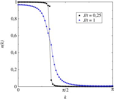
Figure 5: Moment distribution function $n(k)$ at $n_{c}=2/3$ and different values $J/t$. The lines are drawn by ommiting the point at $k=k^{c}_{F}$.

We can get further information from the charge correlation function $C(q)$. The results are depicted in Fig. 6. As we expect for small couplings $J/t$ the function $C(q)$ takes the form of a noninteracting one-dimensional electron gas with a kink at $q=2k_{F}^{c}=n_{c}\pi$. Increasing $J/t$ leads to a cusp-like behaviour of $C(q)$ at $q=2k_{F}^{c}$. In addition, the slope at $q=0$ drops with growing interaction stregth $J/t$. The results displayed in Fig. 6 agree qualitatively with the findings from numerical treatments tsunetsugu_rmp ; moukouri_caron in the examined parameter regime ($J/t\lesssim 1$). This supports the Luttinger liquid picture of our description.

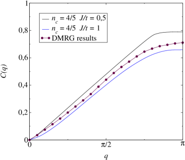
Figure 6: Charge correlation function $C(q)$ of the electrons for different values $J/t$ and band fillings $n_{c}$. Circles are drawn for comparison, taken from xavier_miranda at $J/t=1$ and $n_{c}=4/5$.

The charge correlation function gives us the possibility to derive the parameter $K_{\rho}$ of the Luttinger liquid theory. This parameter is connected to the slope of $C(q)$ at $q=0$ via the relation daul_noack

$$K_{\rho}=\pi\,\frac{\partial C(q)}{\partial q}\,\bigg{|}_{q=0}.$$ (44)

The outcome is depicted in Fig. 7 as a function of the Kondo coupling $J/t$. As we have already mentioned before the slope of $C(q)$ at $q=0$ decreases with growing coupling strength (up to the allowed value of $J/t\lesssim 1$). For vanishing interaction strength $K_{\rho}\to 1$ corresponding to a noninteracting electron gas. This can be understood from the equation for $C(q)$ given in the appendix. Due to the flow equation (33) for the parameter $\gamma_{kq}$ of the electron operator transformation all terms vanish which represent corrections to the charge correlation function of independent electrons. Our findings are in qualitative agreement with recent numerical results from DMRG calculations xavier_miranda . Xavier and Miranda find a minimum of $K_{\rho}(J)$ at $J/t\approx 1.5$. Remember that our largest possible coupling is smaller than $1.5$. Quantitatively our results are always considerably smaller than the values found in ref. xavier_miranda . Another work by Shibata et al. shibata_jp gives results for large $J/t$. In contrast to our findings and to those of Xavier and Miranda xavier_miranda these authors expect $K_{\rho}\to 0$ in the limit $J/t\to 0$.

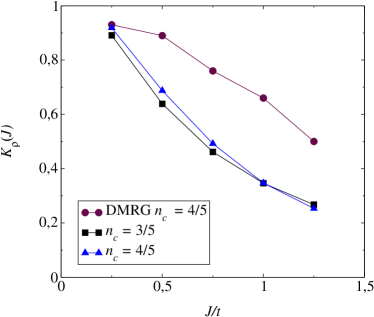
Figure 7: Parameter $K_{\rho}$ as function of $J/t$ for two different band fillings $n_{c}$. Circles are drawn for comparison, data taken from xavier_miranda for $n_{c}=4/5$.

We also considered the dependence of $K_{\rho}$ on the band filling $n_{c}$. This is depicted in Fig. 8. The lower possible value of the band filling is $n_{c}=1/2$ as we do not obtain a solution of the flow equations below this value within the present approach. At small values $J/t$ we find a monotonic decrease by lowering $n_{c}$. Again we find qualitative agreement with Xavier and Miranda xavier_miranda . As we already mentioned in the last discussion our values for $K_{\rho}$ are considerably smaller compared to the numerical data. For larger $J/t$ the behaviour deviates even qualitatively from the numerical DMRG data. Whereas in ref. xavier_miranda for all values of $J/t$ a monotonic increase was obtained on increasing $n_{c}$, we find a maximum in the function $K_{\rho}(n_{c})$.

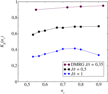
Figure 8: Parameter $K_{\rho}$ as function of the band filling $n_{c}$ for different values $J/t$. Circles are drawn for comparison, data taken from xavier_miranda for $J/t=0.35$.

The magnetic properties of the one-dimensional KLM are significant for the determination of the phase transition from the paramagnetic metallic phase into the ferromagnetic phase. The spin correlation function for the conduction electrons $S_{cc}(q)$ as well as for the local moments $S_{ff}(q)$ show a characteristic increase of the ferromagnetic component $q=0$ on approaching the quantum phase transition.

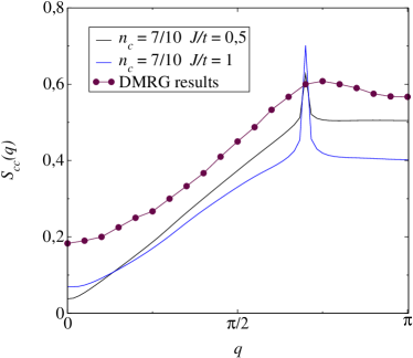
Figure 9: Spin correlation function $S_{cc}(q)$ of the electrons for different values $J/t$ and band fillings $n_{c}$. Circles are drawn for comparison, data taken from moukouri_caron for $J/t=1$ and $n_{c}=7/10$.

The spin correlation function of the electrons $S_{cc}(q)$ is shown in Fig. 9. The strong peak at $q=2k_{F}^{c}$ results from the sharp maximum of the spin correlation function $S(q)$ of the effective model. This can easily be seen from the expression of $S_{cc}(q)$ given in the appendix. Another characteristic is the finite weight of the ferromagnetic component $q=0$ which is directly connected with the occurence of the quantum phase transition. On approaching the critical $J/t$ the maximum of $S_{cc}(q)$ at $q=2k_{F}^{c}$ loses weight in favour of the ferromagnetic component. This behaviour marks the phase transition tsunetsugu_rmp . As we already mentioned the present approach is restricted to values of $J/t\lesssim 1$. These values are too small compared to the value at the transition point which is $J/t\lesssim 2.5$ for $n_{c}=2/3$ shibata_jp . Nevertheless, we observe some tendency towards the magnetic phase transition. As in the case of the charge correlation function we compare our results with numerical data from moukouri_caron . One can clearly see the qualitative agreement between the two approaches, although our findings tend to be smaller than the DMRG results. This is important if one considers the points at $q=0$. The increase of the ferromagnetic component, which signals the tendency towards the quantum phase transition, turns out to be comparably weak.

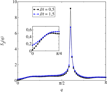
Figure 10: Spin correlation function $S_{ff}(q)$ of the local moments at $n_{c}=3/5$ and different values $J/t$

The situation we have just described is also characteristic for the spin correlation function $S_{ff}(q)$ of the local moments which is drawn in Fig. 10. For small couplings we see that the corrections to the spin correlation function of the effective model $S(q)$ are negligibly small. Even for larger values of $J/t$ we find only small corrections. The vicinity of the ferromagnetic component $q=0$ is shown in the inset. Nevertheless, the qualitative behaviour is once again in agreement with numerical results tsunetsugu_rmp though the values are somewhat larger. Again, the ferromagnetic component gets an increasing weight while the $q=2k_{F}^{c}$ component is suppressed.

IV.3 Dynamic properties

In the last section we have presented the results for static expectation values and correlation functions. We have found that our results are in qualitative agreement with numerical data for small couplings $J/t$. The flow equation method sets us in the position to calculate not only static but also dynamic correlation functions. Within our approach the dynamics of the KLM is described in terms of the effective model (12). Since $\tilde{\cal H}$ is blockdiagonal the dynamics for electrons and local spin moments seperate. The SBMFT allows us, at least approximately, to characterise the excitations of the spin system. The excitations of the KLM are determined by a noninteracting Fermi gas (conduction electrons) and the Schwinger bosons. In this section we shall add new aspects to the results obtained by shibata_tsunetsugu .

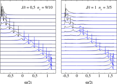
Figure 11: Dynamic correlation functions $A_{+}(k,\omega)$ (black) and $A_{-}(k,\omega)$ (blue) for $k=0$ (up) to $k=\pi$ (down).

We start with the dynamic properties of the conduction electrons. The first quantities we want to consider are the electronic spectral functions $A_{\pm}(k,\omega)$ which can be measured in XPS and inverse XPS experiments. The outcome is shown in Fig. 11. The energy is measured with respect to the Fermi-energy of the conduction electrons $\varepsilon^{c}_{F}=n_{c}\pi/2$. As we have already mentioned in the last section both functions consist of two parts. A coherent quasiparticle-like contribution embodied by the finite peak which has a weight $\tilde{\alpha}_{k}$. Its position is simply given by the renormalized single-particle energies $\tilde{\varepsilon}_{k}$. The incoherent background contains pairs of elementary excitations of the spin system of $\tilde{\cal H}$. This follows directly from Eq. (29) since within the Schwinger boson approach for the effective spin system the corrections to the spectral functions $A_{\pm}(k,\omega)$ are always connected to the creation (annihilation) of pairs of bosons. The coupling to the continuum of Schwinger boson excitations and the results for $\tilde{\gamma}_{kq}$ give rise to the two maxima around the quasiparticle-like peak.

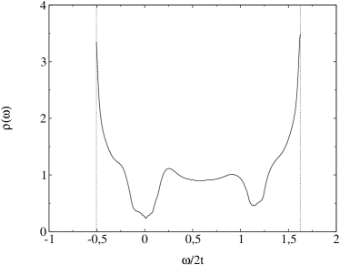
Figure 12: Elektronic density of states $\rho(\omega)$ for $J/t=1$ and $n_{c}=3/5$.

The electronic density of states $\rho(\omega)$ is an important quantity which shows a characteristic behaviour for Luttinger liquids. It is drawn in Fig. 12. Again, the energy is measured with respect to $\varepsilon^{c}_{F}=n_{c}\pi/2$. We find two minima, one in the vicinity of the Fermi level of the conduction electrons, $\omega=0$, the other above the Fermi level. This behaviour follows from the pseudogap-like behaviour of the renormalized single-particle energies $\tilde{\varepsilon}_{k}$. In contrast to our findings DMRG studies from Shibata and Tsunetsugu shibata_tsunetsugu do not yield a minimum but rather a peak structure just below $\omega=0$ indicating the development of a pseudo gap. However, their results were performed at finite temperatures. The Luttinger liquid theory predicts a density of states following $\rho(\omega)\sim|\omega|^{\alpha}$, $0<\alpha<1$ in the vicinity of $\omega=0$. As can be seen from Fig. 12 there is no real vanishing of $\rho(\omega)$ at $\omega=0$. As we are dealing here with a finite system size we are not able to resolve $\rho(\omega)$ near $\omega=0$ and to verify the expected behaviour.

Let us now turn to the magnetic properties. We want to present the results for the dynamic spin structure factors of the electrons $S_{cc}(q,\omega)$ and the local moments $S_{ff}(q,\omega)$. They describe the magnetic excitations of the coupled system and can be measured by inelastic neutron scattering experiments.

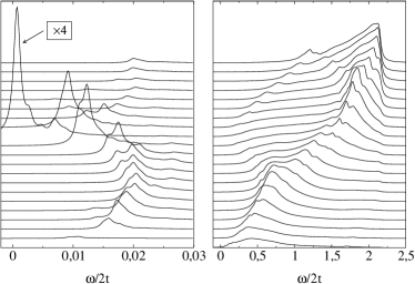
Figure 13: Dynamic spin structure factor of the electrons $S_{cc}(q,\omega)$ for $J/t=1$ and $n_{c}=3/5$, $q=0$ (bottom) and $q=\pi$ (top), Left: Low-energy part. Right: High-energy part.

We begin with the electronic dynamic spin structure factor $S_{cc}(q,\omega)$ which consists of a low- and a high-energy part. Both are discussed seperately. The low energy sector, left panel of Fig. 13, is characterised by the spin part of the effective model $\tilde{\cal{H}}_{S}$, i.e. the continuum of pair excitations of the Schwinger bosons. The dominant contribution is therefore found at $q=2k_{F}^{c}$. It is multiplied by a factor $1/4$ for a better comparison. We also see that there are regions where no excitations are possible. Furthermore, the gap in the spectrum of the elementary excitations $\tilde{\omega}_{q}$ leads to a gap in the low-energy part of $S_{cc}(q,\omega)$. The high-energy sector of $S_{cc}(q,\omega)$ is shown in the right panel of Fig. 13. The spectral weights are about 10 times smaller compared to the weights of the low-energy part. The main contribution arises from electronic particle-hole excitations of the effective model. The specific form of this contribution shows therefore the characteristics of a one-dimensional electron gas: a gapless excitation at $q=2k_{F}^{c}$ and regions between $0<q<2k_{F}^{c}$ where no excitations are possible. In addition to the terms describing pure particle-hole excitations there are also terms involving the elementary excitations $\tilde{\omega}_{q}$ of the effective spin system. They are responsible for the broadening of the structures in the high energy sector of $S_{cc}(q,\omega)$.
The DMRG calculations of Shibata et al. for $S_{cc}(\omega)=\int\frac{dq}{2\pi}S_{cc}(q,\omega)$ showed a small peak at very low energies and a larger double peak structure at higher energies shibata_tsunetsugu . We obtain a similar peak structure, but in contrast to the results of shibata_tsunetsugu the spectral weight of the low energy part is much larger than the spectral weight of the high energy part. This does not agree with the picture of an exhaustion of the electronic low-energy spin degrees of freedom due to singlet formation described by shibata_tsunetsugu .

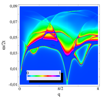
Figure 14: Low energy part of the dynamic spin structure factor $S_{ff}(q,\omega)$ of the local moments for $J/t=1.5$ and $n_{c}=3/5$. The colour function is normalised to the maximum contribution.

Finally we want to discuss the magnetic excitations of the system of local spin moments described by the dynamic spin structure factor $S_{ff}(q,\omega)$. As in the case of the electronic spin structure factor $S_{cc}(q,\omega)$ this function comprises a low- and a high-energy part. The first one is again determined by the elementary excitations $\tilde{\omega}_{q}$ of the spin part of the effective model $\tilde{{\cal H}}_{S}$. It is depicted in Fig. 14 and possesses the same features as the low-energy part of $S_{cc}(q,\omega)$. From this picture we can clearly see the influence of the low-energy spin excitations. The distinct structure at $q=2k_{F}^{c}$ gives rise to the pronounced peak in the static spin correlation function $S(q)$. Once again we point out that the energy scale of these excitations are quite small compared with the effective band width of the electrons. The DMRG results of Shibata et al. for $S_{ff}(\omega)=\int\frac{dq}{2\pi}S_{ff}(q,\omega)$ show a large peak structure at very small energies shibata_tsunetsugu . They assume that this is due to collective spin excitations of the Luttinger-liquid. In our approach the low-energy peak is the result of the continuum of elementary excitations of the effective spin system, which we described in terms of Schwinger bosons.

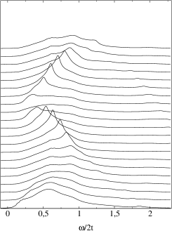
Figure 15: High energy part of the dynamic spin structure factor $S_{ff}(q,\omega)$ of the local moments at $J/t=1.5$ and $n_{c}=3/5$ for $q=0$ (bottom) and $q=\pi$ (top).

The high-energy part of $S_{ff}(q,\omega)$ is shown in Fig. 15. As in the case of $S_{cc}(q,\omega)$ it is mainly determined by particle-hole excitations of the Fermi sea. At larger couplings $J/t$ the elementary spin excitations $\tilde{\omega}_{q}$ lead to the broadening of the peak structure. Shibata et al. obtain a second peak in the high-energy sector of $S_{ff}(\omega)$ shibata_tsunetsugu . Our approach yields a similar structure in the local spin dynamics, although the spectral weight of the high-energy part is much smaller than the spectral weight of the low-energy part.
We further note that $S_{ff}(q,\omega)$ exhibits a finite gap. This is an artifact and due to the approximations that we have made for the spin operator transformation. By taking into account higher correction terms the transformed spin operator of the local spin moment couples to the spin operator of the conduction electrons. This gives rise to a gapless mode in $S_{ff}(q,\omega)$.

V conclusion

In summary, we used the method of continuous unitary transformations (flow equation method) to examine the one-dimensional KLM. The renormalization procedure was employed to integrate out the coupling between conduction electrons and local spin operators. In that way we derived an effective Hamiltonian which consists of an one-dimensional noninteracting electron gas and a Heisenberg chain interacting via an RKKY-like coupling. In order to treat the spin chain we used a Schwinger boson mean field theory (SBMFT). Thereby we were able to calculate static and dynamic correlation functions. The investigation of the electronic momentum distribution revealed a small Fermi surface. We gave arguments, referring to the effective model, why we were not able to obtain the large Fermi surface scenario in our approach. Nevertheless, the static spin and charge correlation functions of the electrons agreed qualitatively with numerical results. In addition we obtained the parameter $K_{\rho}$ of the Luttinger liquid theory and found also qualitative agreement with recent DMRG calculations. The present approach was restricted to parameter regimes $J/t\lesssim 1$. Although the quantum phase transition from the paramagnetic metallic into the ferromagnetic phase takes place at larger values, we observed some tendency to a stronger ferromagnetic component in the static spin correlation functions. The new aspect of this work was the extension of calculations for dynamic properties by means of the flow equation’s method. We showed that the electronic spectral functions comprised a coherent quasiparticle-like peak determined by the renormalized electronic dispersion relation. The coupling to the low-energy excitation of the effective spin model gave an incoherent background comprising two maxima near the quasiparticle-like peaks. Finally, we also computed the magnetic excitations of both the electrons and the local spins. The corresponding spin structure factors always consisted of a low-energy part, determined by the Schwinger boson pair excitations, and a high-energy part, mostly determined by electronic particle-hole excitations. The latter therefore showed the special features of the one-dimensional Fermi surface. The electronic spin structure factor exhibited a gapless mode at $q=2k_{F}^{c}$. Our results for the electronic spin dynamics did not agree with the exhaustion picture described by shibata_tsunetsugu . The gapless mode at $q=2k_{F}^{c}$ should also be seen in the spin structure factor of the local moments. There we argued that further corrections in the spin operator transformation would lead to a gapless mode.

Appendix A correlation functions in the flow equation approach

In this appendix we give the rather lengthy expressions for the static and dynamic correlation functions omitted in the text. These are the static charge correlation function $C(q)$ which reads

$$C(q) =\frac{1}{N}\sum_{kk^{\prime}\sigma\sigma^{\prime}}\langle c^{\dagger}_{k+q\sigma}c_{k\sigma}c^{\dagger}_{k^{\prime}-q\sigma^{\prime}}c_{k^{\prime}\sigma^{\prime}}\rangle\allowdisplaybreaks$$

$$=\frac{2}{N}\sum_{k}\,\tilde{\alpha}^{2}_{k}\,\tilde{\alpha}^{2}_{k+q}\,n_{k+q}(1-n_{k})\allowdisplaybreaks$$

$$+\frac{4}{N^{2}}\sum_{kp}\,\tilde{\alpha}_{k}\,\tilde{\alpha}_{k+q}\,\tilde{\gamma}_{p,k+q}\,\tilde{\gamma}_{p-q,k}\,S(k-p-q)\,n_{k+q}(1-n_{k})+\frac{2}{N^{2}}\sum_{kp}\,\tilde{\alpha}^{2}_{k}\,\tilde{\gamma}^{2}_{k-q,p}\,S(k-p-q)\,n_{k}(1-n_{p})\allowdisplaybreaks$$

$$+\frac{2}{N^{2}}\sum_{kp}\,\tilde{\alpha}^{2}_{k}\,\tilde{\gamma}^{2}_{k+q,p}\,S(k-p+q)\,n_{p}(1-n_{k})+\frac{4}{N^{2}}\sum_{kp}\,\tilde{\alpha}_{k}\,\tilde{\alpha}_{p}\,\tilde{\gamma}_{p+q,k}\,\tilde{\gamma}_{k-q,p}\,S(k-p-q)\,n_{k}(1-n_{p})$$ (45)

The dynamic spin structure factor $S_{cc}(q,\omega)$ of the electrons takes the form

$$S_{cc}(q,\omega) =\int_{-\infty}^{\infty}dt\,\langle{\bf s}_{q}(t)\cdot{\bf s}_{-q}\rangle\,\text{e}^{i\omega t}\allowdisplaybreaks$$

$$=\frac{3}{2N}\sum_{k}\,\tilde{\alpha}^{2}_{k}\,\tilde{\alpha}^{2}_{k+q}\,n_{k+q}(1-n_{k})\,\delta(\omega-\tilde{\varepsilon}_{k}+\tilde{\varepsilon}_{k+q})\allowdisplaybreaks$$

$$-\frac{1}{N^{2}}\sum_{kp}\,\tilde{\alpha}_{k}\,\tilde{\alpha}_{k+q}\,\tilde{\gamma}_{p-q,k}\,\tilde{\gamma}_{p,k+q}\,S(k-p-q)\,n_{k+q}(1-n_{k})\,\delta(\omega-\tilde{\varepsilon}_{k}+\tilde{\varepsilon}_{k+q})\allowdisplaybreaks$$

$$-\frac{1}{2N^{3}}\sum_{kpp^{\prime}}\,\tilde{\alpha}_{k}\,\tilde{\alpha}_{p}\,\tilde{\gamma}_{p+q,k}\,\tilde{\gamma}_{k-q,p}\,(u_{p^{\prime}}v_{p^{\prime}+k-p-q}-v_{p^{\prime}}u_{p^{\prime}+k-p-q})^{2}\,n_{k}(1-n_{p})\delta(\omega-\tilde{\omega}_{p^{\prime}}-\tilde{\omega}_{p^{\prime}+k-p-q}-\tilde{\varepsilon}_{k}+\tilde{\varepsilon}_{p})\allowdisplaybreaks$$

$$+\frac{3}{4N^{3}}\sum_{kpp^{\prime}}\tilde{\alpha}^{2}_{k}\,\tilde{\gamma}^{2}_{k+q,p}\,(u_{p^{\prime}}v_{p^{\prime}+k-p+q}-v_{p^{\prime}}u_{p^{\prime}+k-p+q})^{2}\,n_{p}(1-n_{k})\delta(\omega-\tilde{\omega}_{p^{\prime}}-\tilde{\omega}_{p^{\prime}+k-p+q}-\tilde{\varepsilon}_{p}+\tilde{\varepsilon}_{k})\allowdisplaybreaks$$

$$+\frac{3}{4N^{3}}\sum_{kpp^{\prime}}\tilde{\alpha}^{2}_{k}\,\tilde{\gamma}^{2}_{k-q,p}\,(u_{p^{\prime}}v_{p^{\prime}+k-p-q}-v_{p^{\prime}}u_{p^{\prime}+k-p-q})^{2}\,n_{k}(1-n_{p})\delta(\omega-\tilde{\omega}_{p^{\prime}}-\tilde{\omega}_{p^{\prime}+k-p-q}-\tilde{\varepsilon}_{k}+\tilde{\varepsilon}_{p})\allowdisplaybreaks$$

$$+\frac{1}{2N^{3}}\sum_{kpp^{\prime}}\,\tilde{\alpha}_{k}\,\tilde{\alpha}_{p}\,(\tilde{\gamma}_{k+q,k}\,\tilde{\gamma}_{p-q,p}+\tilde{\gamma}_{k-q,k}\,\tilde{\gamma}_{p+q,p})n_{k}\,n_{p}\,(u_{p^{\prime}}v_{p^{\prime}+q}-v_{p^{\prime}}u_{p^{\prime}+q})^{2}\,\delta(\omega-\tilde{\omega}_{p^{\prime}}-\tilde{\omega}_{p^{\prime}+q})\allowdisplaybreaks$$

$$+\frac{1}{2N^{3}}\sum_{kpp^{\prime}}\,\tilde{\alpha}_{k}\,\tilde{\alpha}_{p}\,(\tilde{\gamma}_{k-q,k}\,\tilde{\gamma}_{p-q,p}+\tilde{\gamma}_{k+q,k}\,\tilde{\gamma}_{p+q,p})n_{k}\,n_{p}\,(u_{p^{\prime}}v_{p^{\prime}+q}-v_{p^{\prime}}u_{p^{\prime}+q})^{2}\,\delta(\omega-\tilde{\omega}_{p^{\prime}}-\tilde{\omega}_{p^{\prime}+q})$$ (46)

Here, it can clearly be seen that the second and third line involves only particle hole excitations of the Fermi sea of the effective model. The last two lines represent the low energy sector of $S_{cc}(q,\omega)$ as they include only pair excitations of Schwinger bosons. On integrating over the energy $\omega$ one obtains the expression for the static spin correlation function $S_{cc}(q)$.

References

- (1) Peter Fulde Electron Correlation in Molecules and Solids, Third Enlarged Edition, Springer-Verlag, Berlin Heidelberg, 1995
- (2) A. C. Hewson The Kondo Problem to Heavy Fermions, Cambridge University Press, Cambridge, 1993
- (3) M. Troyer, D. Würtz, Phys. Rev. B 47, 2886 (1993)
- (4) Hirokazu Tsunetsugu, Manfred Sigrist, Kazuo Ueda, Rev. Mod. Phys. 69, 809 (1997) and references therein
- (5) Hirokazu Tsunetsugu, Kazuo Ueda, Manfred Sigrist, Phys. Rev. B 47, 8345 (1993)
- (6) Naokazu Shibata, Kazuo Ueda, J. Phys.: Condens. Matter 11, R1 (1999)
- (7) J.C. Xavier, E. Novais, E. Miranda, Phys. Rev. B 65, 214406 (2002)
- (8) S. Moukouri, L. Caron, Phys. Rev. B 52, R15723 (1995)
- (9) S. Caprara, A. Rosengren, Europhys. Lett. 39, 55 (1997)
- (10) N. Shibata and H. Tsunetsugu J. Phys. Soc. Jpn. 68, 3138 (1999)
- (11) Clare C. Yu, Steven R. White, Phys. Rev. Lett. 71, 3866 (1993)
- (12) Graeme Honner, Miklos Gulacsi, Phys. Rev. Lett. 78, 2180 (1997); Graeme Honner, Miklos Gulacsi, Phys. Rev. B 58, 2662 (1998)
- (13) I. P. McCulloch, A. Juozapavicius, A. Rosengren, M. Gulacsi, Phys. Rev. B 65, 052410 (2002)
- (14) Eugene Pivovarov, Qimiao Si, Phys. Rev. B 69, 115104 (2004)
- (15) S. Doniach, Physica B 91, 231 (1977)
- (16) J. M. Luttinger, Phys. Rev. 119, 1153 (1960)
- (17) J. Voit, Rep. Prog. Phys. 57, 977 (1994)
- (18) J. R. Schrieffer, P. A. Wolff, Phys. Rev. 149, 491 (1966)
- (19) N. Shibata et al. cond-mat/0503476
- (20) Franz Wegner, Ann. Physik 3, 77 (1994)
- (21) S. Głazek, K. G. Wilson, Phys. Rev. D 48, 5863 (1994)
- (22) J. Stein, Eur. Phys. J. B 12, 5 (1999)
- (23) P. Lenz, F. Wegner, Nucl. Phys. B 482 693 (1996); M. Ragwitz, F. Wegner, Eur. Phys. J. B 8, 9 (1999); A. Mielke, Ann. Physik 6, 215 (1997); A. Mielke Europhys. Lett. 40 (2), pp. 195-200 (1997);
- (24) C. Heidbrink, G. Uhrig, Phys. Rev. Lett. 88, 146401 (2002); C. Heidbrink, G. Uhrig, Eur. Phys. J. B 30, 443 (2002); S. Kehrein, Phys. Rev. Lett. 83, 4914 (1999)
- (25) G. Uhrig, Phys. Rev. B 57, R14004 (1998); C. Raas, U. Löw, G. Uhrig, Phys. Rev. B 65, 144438 (2002); S. Kehrein, A. Mielke, Ann. Physik 6 90 (1997); S. Kehrein, A. Mielke, P. Neu, Z. Phys. B 99 269 (1996)
- (26) Daniel P. Arovas, Assa Auerbach, Phys. Rev. B 38 316 (1988); Assa Auerbach, Daniel P. Arovas, Phys. Rev. Lett. 61 617 (1988)
- (27) A. E. Trumper, L. O. Manuel, C. J. Gazza, H. A. Ceccatto, Phys. Rev. Lett. 78, 2216 (1997)
- (28) H. A. Ceccatto, C. J. Gazza, A. E. Trumper, Phys. Rev. B 47, 12 329 (1993)
- (29) S. Daul, R.M. Noack, Phys. Rev. B 58, 2635 (1998)
- (30) J.C. Xavier, E. Miranda, Phys. Rev. B 70, 075110 (2004)
- (31) S. Sachdev, Phys. Rev. B 45, 12 377 (1992)