Cooperative Dynamics in a Network of Stochastic Elements with Delayed Feedback

Abstract

Networks of globally coupled, noise activated, bistable elements with connection time delays are considered. The dynamics of these systems is studied numerically using a Langevin description and analytically using (1) a Gaussian approximation as well as (2) a dichotomous model. The system demonstrates ordering phase transitions and multi-stability. That is, for a strong enough feedback it exhibits nontrivial stationary states and oscillatory states whose frequencies depend only on the mean of the time delay distribution function. Other observed dynamical phenomena include coherence resonance and, in the case of non-uniform coupling strengths, amplitude death and chaos. Furthermore, an increase of the stability of the trivial equilibrium with increasing non-uniformity of the time delays is observed.

I Introduction

Due to its relevance for a variety of scientific disciplines such as physics, chemistry, biology, economics and social sciences, the study of collective phenomena in extended stochastic systems with long range interaction has been of great interest in recent years and various techniques based on Langevin, Fokker-Planck and master equations have been conceived to explore their dynamics.

An effective and simple model for the study of noise induced collective phenomena is the globally coupled network of stochastically driven bistable elements. Indeed, the cooperative dynamics of these systems has been the subject of many studies and its relevance for critical phenomena (Dawson, 1983), spin systems (Jung et al., 1992), neural networks (Koulakov et al., 2002; Camperi and Wang, 1998; Sompolinsky, 1986), genetic regulatory networks (Gardner et al., 2000) and decision making processes in social systems (Zanette, 1997) has been pointed out.

For the sake of simplicity it has traditionally been assumed that the interactions in these networks are instantaneous. However, in recent years it has been realized that time delays due to finite transmission and processing speeds are 1) significant compared to the dynamical time scales of the system and 2) often change fundamentally its dynamical properties (Reddy et al., 1998; Nakamura et al., 1994; Bressloff and Coombes, 1998; Choi and Huberman, 1985).

Thus, in this paper the generic model of globally coupled bistable elements is extended by time delayed couplings and its collective dynamics is studied numerically and analytically.

The properties of globally coupled dynamical units, relevant for system such as arrays of lasers (Wiesenfeld et al., 1990) and Josephson junctions (Wiesenfeld and Hadley, 1989), have been explored in many studies (see also Yeung and Strogatz, 1999; Van den Broeck and Parrondo, 1994; Jung et al., 1992; Kuramoto, 1991; Shiino, 1987; Desai and Zwanzig, 1978). Desai and Zwanzig (1978), for instance, studied the synchronization of noise activated bistable oscillators with instantaneous coupling and derived from the Fokker-Planck equation for the joint probability distribution of the oscillators an exact mean field model (DZ-model) in the thermodynamic limit $N\to\infty$, where $N$ is the number of network elements. Beyond a critical coupling strength this system displays a second order phase transition to an ordered nontrivial stationary state. The effect of uniform interaction delays in a globally coupled network of phase oscillators has been explored by Yeung and Strogatz (1999), and Tsimring and Pikovsky (2001) studied the dynamics of a single noise activated bistable element with delayed feedback. Combining the properties of these two systems, Huber and Tsimring (2003) studied the properties of a globally coupled network of noisy bistable elements with uniform delays and derived a dichotomous mean field model based on the delay-differential master equation. Although for numerous systems the assumption of uniform time delays is justified (e.g. Salami et al., 2003; Paulsson and Ehrenberg, 2001), most systems have time delays distributed over an interval rather than concentrated at a point (see Atay, 2003). Thus, after a discussion of the dynamical properties of the network with uniform delays, the generalized case of distributed time delays is studied.

This paper which is an extended version of Huber and Tsimring (2003) is organized as follows: In the next Section the bistable-element-network is discussed for the case of uniform time delays. Two mean field models, namely the DZ-model (which for Gaussian processes reduces to the Gaussian approximation) and the dichotomous model, are compared with the Langevin dynamics and their scopes of application are determined. The phenomenon of coherence resonance is discussed and a complete bifurcation analysis of the trivial equilibrium is carried out using a center manifold reduction. In Sect. III the system dynamics is discussed for a discrete bimodal delay distribution. Then, in Sect. IV the model is further generalized, so that the mean field dynamics of a system with an arbitrary time delay distribution can be described. Finally, in Sect. V we introduce nonuniform coupling strengths which lead to new dynamical properties, such as amplitude death and chaos.

II Uniform delays

II.1 Langevin model

The prototypical system considered here is modeled by a set of $N$ Langevin equations, each describing the overdamped stochastically driven motion of a particle in a bistable potential $V=-x^{2}/2+x^{4}/4$, whose symmetry is distorted by the time delayed coupling to all network elements,

$$\dot{x}_{i}(t)=x_{i}(t)-x_{i}(t)^{3}+\frac{\varepsilon}{N}\sum_{j=1}^{N}x_{j}(t-\tau)+\sqrt{2D}\xi(t),$$ (1)

where $\tau$ is the time delay, $\varepsilon$ is the coupling strength of the feedback and $D$ denotes the variance of the Gaussian fluctuations $\xi(t)$, which are mutually independent and uncorrelated $\langle\xi_{i}(t)\xi_{j}(t^{\prime})\rangle=\delta_{ij}\delta(t-t^{\prime})$.

The global coupling leads to an asymmetry of the local potential; that is, a positive feedback increases the probability for an element to be in the potential well in which the majority of elements were at time $t-\tau$. The inverse holds for a negative feedback.

System (1) is explored numerically. In this paper, the numerical simulations are carried out using an Euler method. If not otherwise indicated the time-step and the number of elements are $\Delta t=0.01-0.05$ and $N=2500$.

Our interest is mainly focused on the cooperative interactions of the individual network elements, i.e., on the dynamics of the mean field $X=N^{-1}\sum_{j=1}^{N}x_{j}$. For $\varepsilon=0$, the elements are decoupled from each other. They jump from one potential well to the other randomly and independently of each other. Therefore, in this case the mean field $X=0$. For small $|\varepsilon|$, the mean field remains zero. At a certain $\varepsilon=\varepsilon_{\rm st}>0$ which depends on the noise intensity $D$, but is independent of the time delay, the system undergoes a second order (continuous) phase transition and adopts a non-zero stationary mean field.

For a negative feedback, a transition to a periodically oscillating mean field solution is observed at a certain $\varepsilon=\varepsilon_{\rm osc-}<0$. Here and for the rest of this paper a $(-/+)$ index means that the corresponding value is associated with a negative/positive feedback.

Above a certain noise level $D_{H}$ the transition at $\varepsilon_{\rm osc-}$ is second order as well. However, for $D<D_{H}$ the system exhibits a first order (discontinuous) transition associated with hysteretic behavior. The noise intensity $D_{H}$ depends on the time delay and is $D_{H}=0.07$ for $\tau=100$.

For large time delays $\tau\gg\tau_{K}$ ($\tau_{K}$ is the inverse Kramers escape rate from one well into the other (Hänggi et al., 1990; Kramers, 1940)), depending on the initial state the system adopts one of many accessible oscillatory states featuring different periods. Even for a positive feedback, besides the stationary solution several oscillatory states with periods $T\lesssim\tau$ are observed for $\varepsilon>\varepsilon_{\rm osc+}\gtrsim\varepsilon_{\rm st}$. If the feedback is negative, the system only has oscillatory nontrivial solutions. The observed periods are $T\lesssim 2\tau$ for $\varepsilon<\varepsilon_{\rm osc-}$.

The basic dynamical states accessible by the system are illustrated in Figs. 1 and 2, where the evolution of a single network element and the mean field are shown for different coupling strength.

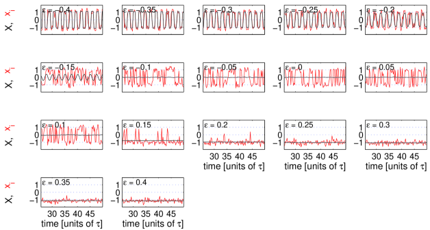
Figure 1: Dynamics of a single network oscillator $x_{i}$ and the network mean field $X$ for different coupling strength $\varepsilon$. The noise strength and the time delay is $D=0.1$ and $\tau=100$, respectively. For $\varepsilon<\varepsilon_{\rm osc}=-0.13$ the mean field adopts a state of periodic oscillations. In the range $\varepsilon_{\rm osc}<\varepsilon<\varepsilon_{\rm st}=0.11$ the trivial equilibrium is stable. Finally, for $\varepsilon>\varepsilon_{\rm st}$ the system adopts a non-zero stationary state.

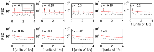
Figure 2: For $\varepsilon\leq 0$, same as in Fig. 1, but in the frequency domain.

II.2 Gaussian approximation

A mean field description for the dynamics of a globally coupled set of thermally activated bistable elements with instantaneous interactions was proposed by Desai and Zwanzig (1978). For the sake of simplicity, we refer to this mean field description as the DZ-model. This model consists of a hierarchy of equations for the cumulants of the distribution function derived from the Fokker-Planck equation for the joint probability density function of all elements. Expressed in terms of moments $M_{n}\;\{n=1\ldots\infty\}$ the hierarchy assumes the simple form,

$$\dot{M}_{n}=X(t-\tau)[4DM_{n-2}+\varepsilon M_{n-1}]+M_{n}-M_{n+2},$$ (2)

where $M_{-1}=0$ and $M_{0}=1$.

For large noise intensities, when the statistics of the individual elements are approximately Gaussian the hierarchy can be truncated (Gaussian approximation (see also Pikovsky et al., 2002)). Applying this approach to our delayed feedback system, the evolution of the mean field $X$ is, in the Gaussian approximation, described by the following set of equations,
$\displaystyle\dot{X}(t)$ $\displaystyle=$ $\displaystyle X(t)-X^{3}(t)-3X(t)V(t)+\varepsilon X(t-\tau),$ $\displaystyle\frac{1}{2}\dot{V}(t)$ $\displaystyle=$ $\displaystyle V(t)-3X^{2}(t)V(t)-3V^{2}(t)+D,$ where $V=M_{2}-M^{2}_{1}=N^{-1}\sum_{i=1}^{N}(x_{i}-X)^{2}$ is the variance.

To compare the theoretical predictions of the Gaussian approximation (II.2) with the Langevin model (1) we determine the maximum of the main peak in the power spectrum $P_{\rm peak}$ (see Fig. 2). The evolution of the peak power as a function of the coupling strength can be used to study the Hopf bifurcation which describes the transition to the oscillatory mean field regime. The pitchfork bifurcation describing the transition to the stationary mean field state is characterized by the dependence of the temporal mean of the mean field $\langle X\rangle_{t}$ on the coupling strength. Fig. 3 shows the peak power $P_{\rm peak}$ and the temporal mean $\langle X\rangle_{t}$ as a function of the coupling strength $\varepsilon$ for three different noise temperatures $D$.

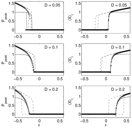
Figure 3: The peak power $P_{\rm peak}$ and the temporal mean $\langle X\rangle_{t}$ as a function of the coupling strength for the Langevin model (crosses), the Gaussian approximation (dashed line), where the double line indicates hysteretic behavior, and the dichotomous theory (solid line). The noise strengths is indicated in the upper right corner of each panel. The time delay is $\tau=100$. For $X=0$ and $D=0.05\,,0.1\,,0.2$ the Kramers times are $\tau_{K}=659.4\,,54.1\,,15.5$.

The phase diagrams of these models are shown in Fig. 4 in the $(D,\varepsilon)$-parameter plane. Fig. 3 shows that away from the transition points the Gaussian approximation correctly describes the Langevin dynamics. However, near the bifurcation points the system dynamics is strongly non-Gaussian even for strong noise. Indeed, while the Gaussian approximation predicts that both bifurcations are first order transitions (associated with hysteretic behavior) over the entire noise range considered in this study (see Fig. 4), the Langevin model produces first order transitions only for $D<0.7$.

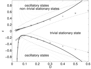
Figure 4: Phase diagram for $\tau=100$ of the Langevin model (crosses), the Gaussian approximation (dashed lines) and the dichotomous theory (solid lines and dotted lines). The solid line and the dotted line respectively depict the primary solution and the higher order solutions of Eq. (15) and (16). Phases separated by double lines indicate hysteretic behavior. For $X=0$ and $D<0.3$ the Kramers time is $\tau_{K}>10$.

The inclusion of higher order cumulant equations leads only to a slow convergence toward the true solution of the Langevin model. This is illustrated in Fig. 5. Thus, near the transition points the DZ-model does not significantly simplify the Langevin description and the critical parameters for the transition cannot be determined analytically.

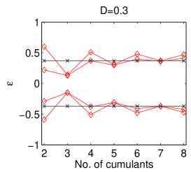
Figure 5: The critical coupling of the Hopf bifurcation $(\varepsilon_{\rm osc}^{1}<0)$ and the pitchfork bifurcation $(\varepsilon_{\rm st}>0)$, respectively. Compared are the critical couplings resulting from the Langevin model (crosses) and the predictions of the DZ-theory (diamonds) including different numbers of cumulants. For an even number of cumulants the DZ-theory predicts hystertic behavior which is not seen in the Langevin dynamics.

II.3 Dichotomous Model

In order to describe the dynamics of the system near the bifurcation points we apply a dichotomous (i.e. two-state) approximation, which is complementary to the Gaussian approximation and which is valid in the limit of small noise, when the characteristic Kramers transition time is $\tau_{K}\gg 1$, and small coupling strengths. The dichotomous theory neglects intra-well fluctuation of $x_{i}$. Thus, in the limit of small coupling, each bistable element can only take the values $s_{1,2}=\pm 1$. The collective dynamics of the entire network can then be described by the master equations for the occupation probabilities of these states $n_{1,2}$. This approach has been successfully used in studies of stochastic and coherence resonance (e.g. McNamara and Wiesenfeld, 1989; Gammaitoni et al., 1998; Jung et al., 1992; Tsimring and Pikovsky, 2001). For example, using this approach Jung et al. (1992), found nontrivial stationary mean field solutions in a globally coupled delay-free network of bistable elements.

The dynamics of a single element is determined by the hopping rates $p_{12}$ and $p_{21}$, i.e., by the probabilities to hop over the potential barrier from $s_{1}$ to $s_{2}$ and from $s_{2}$ to $s_{1}$, respectively. In a globally coupled system, $n_{1,2}$ and $p_{12,21}$ are identical for all elements and the master equations for the occupation probabilities read,

$$\dot{n}_{1} = -p_{12}n_{1}+p_{21}n_{2}$$ (4)

$$\dot{n}_{2} = \;\;\,p_{12}n_{1}-p_{21}n_{2}.$$ (5)

The hopping probabilities $p_{12,21}$ are given by Kramers’ transition rate (Kramers, 1940) for the instantaneous potential well,

$$p^{12,21}_{\rm K}=\frac{\sqrt{U^{\prime\prime}(x_{m})U^{\prime\prime}(x_{0})}}{2\pi}\exp\left(\frac{-\Delta U}{D}\right)\;,$$ (6)

where $x_{m}$ and $x_{0}$ are the positions of the potential minima and the top of the potential barrier, respectively. For our system, in the limit of small noise $D$ and coupling strength $\varepsilon$, they read (cf. Tsimring and Pikovsky, 2001),

$$p_{12,21}=\frac{\sqrt{2\mp 3\alpha_{1}}}{2\pi}\exp\left(-\frac{1\mp 4\alpha_{1}}{4D}\right),$$ (7)

where $\alpha_{1}=\varepsilon X(t-\tau)$.

As discussed above, the Langevin system either adopts a stationary or an oscillatory mean field state in the limit $t\to\infty$. Let us first consider the stationary case $\dot{n}_{1,2}=0$. Making use of the probability conservation $n_{1}+n_{2}=1$, the occupational probabilities $n_{1,2}$ are given by

$$n_{1,2}=\frac{p_{21,12}}{p_{12}+p_{21}}\;.$$ (8)

Then, in the dichotomous approximation with $s_{1,2}=\pm 1$, the mean field $X=s_{1}n_{1}+s_{2}n_{2}$ reads

$$X=n_{2}-n_{1}=\frac{p_{12}-p_{21}}{p_{12}+p_{21}}\;.$$ (9)

Substituting the hopping probabilities (7) into this equation yields the transcendental equation for the mean field magnitude

$$X=\frac{\sqrt{2-3\varepsilon X}\exp\left(\varepsilon X/D\right)-\sqrt{2+3\varepsilon X}\exp\left(-\varepsilon X/D\right)}{\sqrt{2-3\varepsilon X}\exp\left(\varepsilon X/D\right)+\sqrt{2+3\varepsilon X}\exp\left(-\varepsilon X/D\right)}$$ (10)

This equation always has a trivial solution $X=0$, but for $\varepsilon>\varepsilon_{\rm st}$ it also has a pair of nontrivial solutions $X=\pm A$. It is easy to find $A(\varepsilon)$ for a fixed $D$ numerically using (10). The critical value $\varepsilon_{\rm st}$ as a function of $D$ for the pitchfork bifurcation, indicating the transition to a nontrivial stationary state, can be found analytically by expanding the r.h.s. of Eq. (10) at small $X$. This yields the following expression

$$\varepsilon_{\rm st}=\frac{4D}{4-3D}\;.$$ (11)

Let us now turn to the general case when $X$ is allowed to be a function of time. Again, making use of the probability conservation and the expression for the dichotomous mean field $X=n_{2}-n_{1}$ we find the equation,

$$\dot{X}(t)=p_{12}-p_{21}-(p_{21}+p_{12})X(t),$$ (12)

where the hopping probabilities $p_{12,21}$ have the same functional form as in Eq. (7), but now depend on the delayed mean field $X(t-\tau)$ rather than $X(t)$.

To investigate the stability properties of the system, Eq. (12) is linearized about zero,

$$\dot{X}(t)=\frac{\sqrt{2}}{\pi}\exp(-1/4D)\left(\varepsilon\frac{4-3D}{4D}X(t-\tau)-X(t)\right)\;.$$ (13)

The characteristic equation for the complex eigenvalue $\lambda$ is found by making the ansatz $X\propto\exp(\lambda t)$. It reads,

$$\lambda=\frac{\sqrt{2}}{\pi}{\rm e}^{-1/4D}\left(\frac{\varepsilon(4-3D)}{4D}{\rm e}^{-\lambda\tau}-1\right).$$ (14)

The trivial equilibrium loses its stability and undergoes a Hopf bifurcation indicating the transition to an oscillatory mean field state when the real part of the complex eigenvalue becomes positive. Therefore, the properties of the corresponding instabilities (i.e. frequencies and coupling strengths at the bifurcation points) can be found by substituting $\lambda=\mu+{\rm i}\omega$ into Eq. (14), separating real and imaginary parts and setting $\mu=0$. This yields the following set of equations,

$$\omega\tau = -\frac{\sqrt{2}}{\pi}\exp(-1/4D)\tau\tan\omega\tau$$ (15)

$$\varepsilon_{\rm osc} = \frac{\varepsilon_{\rm st}}{\cos\omega\tau}.$$ (16)

This set of equations has a multiplicity of solutions, indicating that multi-stability occurs in the globally coupled system beyond a certain coupling strength. For finite time delays and positive coupling, besides the stationary solution, several oscillatory states with periods $T_{k}$ close to but slightly larger than $\tau/k$ exist for $\varepsilon>\varepsilon^{k}_{\rm osc+}\;\;\{k=1,2,\ldots\}$, where the transition points are ordered as follows, $0<\varepsilon_{\rm st}<\varepsilon^{1}_{\rm osc+}<\varepsilon^{2}_{\rm osc+}\ldots$ If the feedback is negative, the system has oscillatory solutions with periods $T_{l}$ close to but slightly larger than $2\tau/(2l+1)$ for $\varepsilon<\varepsilon^{l}_{\rm osc-}\;\;\{l=0,1,\ldots\}$, where $0>\varepsilon^{0}_{\rm osc-}>\varepsilon^{1}_{\rm osc-}\ldots$ In the limit of large time delays $\tau\to\infty$, the transition points $\varepsilon^{k}_{\rm osc+}\to\varepsilon_{\rm st}$ and $\varepsilon^{l}_{\rm osc-}\to\varepsilon^{0}_{\rm osc-}=-\frac{4D}{4-3D}$ with the corresponding periods being $T_{k}\to\tau/k$ and $T_{l}\to 2\tau/(2l+1)$, respectively.

In order to compare the predictions of the dichotomous model with the Langevin dynamics, the peak power $P_{\rm peak}$ and the temporal mean $\langle X\rangle_{t}$, resulting from the dichotomous theory, are also plotted in Fig. 3. The phase diagram for the dichotomous theory is shown in Fig. 4.

Fig. 3 and 4 show that the dichotomous theory agrees with the Langevin dynamics quite well for small noise in the range $D\approx 0.07-0.3$ in the neighborhood of the bifurcation points. The theory also correctly describes the bifurcation type. Indeed, the dichotomous theory predicts accurately the noise strength $D_{\rm H}$ ($=0.07$ for $\tau=100$) at which the Hopf bifurcation changes from supercritical (second order) to subcritical (first order). However, for very small $D$ the Kramers time becomes very large, and the accuracy of numerics becomes insufficient for a comparison with the theory.

II.4 Complete bifurcation analysis

A complete bifurcation analysis of the trivial solution $X=0$ of Eq. (13) in the $(D,\varepsilon,\tau)$-parameter space can be accomplished by carrying out a center manifold reduction (see e.g. Chow and Hale, 1982; Faria and Magalhães, 1995); that is, the normal form coefficients of the bifurcations in our dichotomous mean field model can be expressed in terms of the system parameters.

For a general class of delay differential equations of the form,

$$\dot{x}(t) = x(t)+\gamma_{1}x(t-\tau)+\gamma_{2}x(t)^{3}+\gamma_{3}x(t)^{2}x(t-\tau)$$ (17)

$$+\gamma_{4}x(t)x(t-\tau)^{2}+\gamma_{5}x(t-\tau)^{3},$$

such a reduction to normal forms of the pitchfork and Hopf bifurcations has been carried out in Refs. (Giannakopoulos and Zapp, 1999; Redmond et al., 2002). If we cast the equation for the mean field dynamics of our model in this form, we can use the results in Refs. (Giannakopoulos and Zapp, 1999; Redmond et al., 2002) to determine the functional dependence of the normal form coefficients on the parameters $D$, $\varepsilon$, and $\tau$. This can be achieved by a series expansion of Eq. (12) up to the third order and rescaling of time.

The normal form of the pitchfork bifurcation reads

$$\dot{z}=az+bz^{3},$$ (18)

where $z$ is a coordinate on the center manifold. The normal form coefficients are

$$a = \frac{\varepsilon-\varepsilon_{\rm st}}{\varepsilon_{\rm st}(1-\tau_{0})}$$ (19)

$$b = \frac{B_{1}-12DB_{2}}{384(1-\tau_{0})D^{3}},$$ (20)

where $B_{1}=\varepsilon^{3}(81D^{3}+108D^{2}+144D-64)$, $B_{2}=\varepsilon^{2}(9D^{2}+24D-16)$ and $\tau_{0}=-\sqrt{2}\exp(-1/4D)\tau/\pi$. Setting $a=0$ and solving Eq. (19) for $\varepsilon$ we again find the critical coupling of Eq. (11). One can show that $b<0$ for $D>0$ and $\varepsilon=\varepsilon_{\rm st}$ (i.e. $a=0$). Consequently, the pitchfork bifurcation at $\varepsilon_{\rm st}$ is always supercritical. The stability diagram resulting from center manifold reduction for the pitchfork bifurcation is shown in Fig. 6.

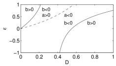
Figure 6: Stability diagram for the trivial equilibrium resulting from the analysis of the pitchfork bifurcation. The solid and the dashed lines respectively depict the b=0 and a=0 contour lines. The stability diagram for the pitchfork bifurcation is time delay independent.

The normal form of the Hopf bifurcation in polar coordinates $r$ and $\theta$ on the center manifold reads

$$\dot{r}=\mu r+\alpha r^{3}\ ,\;\;\dot{\theta}=\omega+\rho r^{2}.$$ (21)

The coefficients determining the stability of the trivial equilibrium and the order of the Hopf bifurcation are $\mu$ and $\alpha$ (Strogatz, 2000). Expressed in system parameters, they read

$$\mu = \left(\frac{\varepsilon}{\varepsilon_{\rm st}}-\frac{1}{\cos\varphi}\right)\left(\frac{1-\tau_{0}}{(1-\tau_{0})^{2}+\varphi^{2}}-\frac{\sin\varphi}{2}\right),$$ (22)

$$\alpha = \frac{B_{1}B_{3}-B_{2}(1-3\tau_{0}+2\cos^{2}\varphi)}{128([1-\tau_{0}]^{2}+\varphi^{2})D^{2}},$$ (23)

where $B_{3}=(\cos^{2}\varphi-\tau_{0})/(4D\cos\varphi)$, $\varphi=\omega_{0}\tau_{0}$ and $\omega_{0}=\tan\varphi$.

Setting $\mu=0$ and solving Eq. (22) for $\varepsilon$ yields the critical coupling as a function of the noise strength $\varepsilon_{\rm osc}(D)$ which coincides with Eq. (16). Setting the first Lyapunov coefficient $\alpha=0$, we can find $\varepsilon_{\alpha=0}(D)$. The two functions $\varepsilon_{\rm osc}(D)$ and $\varepsilon_{\alpha=0}(D)$ intersect at a noise level $D_{\rm H}$ denoting the parameter values for which the Hopf bifurcation changes from supercritical to subcritical. The stability diagram resulting from the analysis of the Hopf bifurcation is shown in Fig. 7.

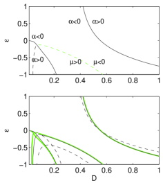
Figure 7: Primary solutions of $\mu=0$ (Eq. 22) and $\alpha=0$ (Eq. 23) in the $(\varepsilon,D)$-parameter-space. Upper panel: The boundaries $\mu=0$ (dashed line) and $\alpha=0$ (solid line) for a system with $\tau=100$. The black dashed line and the gray dashed line depicts the parameter values of the subcritical and supercritical Hopf bifurcation, respectively. The lower panel shows the same curves for a system with $\tau=10$ (dashed line), $\tau=100$ (black solid line) and $\tau=1000$ (gray solid line).

Let us now discuss the bifurcation properties in the limit of large and small time delays as well as vanishing noise and compare them with those of a single oscillator system. The critical coupling $\varepsilon_{\rm st}$ of the pitchfork bifurcation is time delay independent and goes to zero for vanishing noise. However, the critical coupling of the Hopf bifurcation depends on the time delay (see lower panel in Fig. 7). As the time delay increases, the maximum of the primary Hopf bifurcation line $\varepsilon_{\rm osc-}^{1}$ approaches the origin in the $(\varepsilon,D)$ plane meaning that oscillations may occur at an arbitrary small feedback strength for the properly tuned noise level. This should be contrasted to the dynamics of a single noise-free oscillator with time-delayed feedback that only exhibits oscillations at strong negative feedback $(\epsilon<-1)$. For very small time delays $\tau\to 0$, the critical coupling strength $\varepsilon^{l,k}_{\rm osc\mp}\to\mp\infty$.

II.5 Coherence resonance and system size effects

The system studied in this paper exhibits the phenomenon of coherence resonance (e.g. Kiss et al., 2003; Miyakawa and Isikawa, 2002; Pikovsky and Kurths, 1997; Sigeti and Horsthemke, 1989) and array-enhanced resonance (Pikovsky et al., 2002; Zhou et al., 2001).

Let us discuss this in turn. If our system adopts an oscillatory state, the double-well potentials of the elements are tilted asymmetrically, due to their coupling to the delayed mean field; that is, the potential barriers separating the two wells are periodically rising the lowering. If the period of this oscillation $T$ matches the time scale $\tau_{\rm K}$ of the noise-induced inter-well fluctuation, i.e., if the mean field oscillations synchronize with the hopping rate, we can expect that the number of elements contributing to the oscillation and consequently the order of the oscillatory state reach a maximum. In this spirit the time scale matching condition for such a synchronization, which is given through

$$2\tau_{\rm K}=T,$$ (24)

is a reasonable condition for the maximum order of the oscillatory state (Gammaitoni et al., 1998).

To quantify the order (i.e. coherence) of the oscillatory state we introduce the coherence parameter $\beta=H\omega_{\rm peak}/\Delta\omega$, where H is the height of the main spectral peak at $\omega_{\rm peak}$ and $\Delta\omega$ is its halfwidth. Using the Langevin model (1), the coherence measure $\beta$ is determined as a function of the noise strength and in Fig. 8 compared for systems of different size $N$.

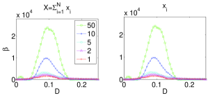
Figure 8: The coherence of the oscillatory states $\beta$ as a function of the noise strength $D$ for systems of different size $N$. The time delay and the coupling strength are $\tau=100$ and $\varepsilon=-0.2$, respectively. Left panel: The coherence of the mean field oscillations. Right panel: The coherence of a single element $x_{i}$ out of the $N$ network elements.

Clearly, the coherence curves have a maximum. The noise strength maximizing the coherence is $D_{\rm S}\approx 0.08$. This noise strength can also be derived from the time scale matching condition in Eq. (24). The Kramers time $\tau_{\rm K}=1/p$ is given through Eq. (7) and the period of the oscillations $T$ beyond the critical coupling can be determined numerically. In Fig. 9 the two time scales are plotted as function of the noise strength. The curves intersect at D=0.08 substantiating the consistency of theory and Langevin model.

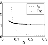
Figure 9: The Kramers time $\tau_{\rm K}$ and the half the period of the mean field oscillations (in units of the time delay) as a function of the noise strength. The parameters are $\tau=100$ and $\varepsilon=-0.2$.

The resonance curves in Fig. 8 show that the coherence of the oscillatory states increases with increasing $N$, a property which was reported for other systems and is sometimes referred to as array-enhanced resonance (Zhou et al., 2001). Interestingly, the enhancement of the temporal regularity with increasing system size is only observed for macroscopic mean field oscillations, while the inverse holds for “subcritical coherence”. That is, the coherence observed in the power spectra of subcritical mean field fluctuations (i.e., for $|\epsilon|<|\epsilon_{\rm osc\pm}|)$ decays inversely proportional to the number of elements in the network, and becomes negligible for $N>10$. This is show in Fig. 10. Qualitatively, the same dependency on the system size is found if the delayed average does not include the delayed element itself, i.e., the element $x_{i}$ is coupled to $X_{i}(t-\tau)=\sum^{N-1}_{{j=1},{j\neq i}}x_{j}$.

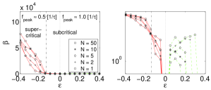
Figure 10: The coherence $\beta$ as function of the coupling strength. For $\varepsilon<0$ and $\varepsilon>0$ the spectral peak frequency is $f_{\rm peak}=\omega_{\rm peak}/2\pi\approx 0.5\;1/\tau$ and $f_{\rm peak}\approx 1.0\;1/\tau$, respectively. The dash-dotted vertical line depicts $\varepsilon^{1}_{\rm osc-}$ and consequently separates domain of the macroscopic (i.e. supercritical) mean field oscillations from the domain of subcritical coherence. The right panel shows the same as the left, but has a logarithmic scale for $\beta$, which helps to uncover the weak subcritical coherence properties.

III Two delays

III.1 Langevin model

We want to generalize the above system by introducing multiple time delays and non-uniform coupling terms. Let us carry out the generalization progressively and study first the dynamics of a bistable element network with a discrete bimodal delay distribution (i.e. with two time delays) and uniform coupling. Assuming that the time delay of the interaction between two elements is entirely determined by the “transmitting” element the system dynamics is described by the following set of Langevin equations,

$$\dot{x_{i}}=x_{i}-x_{i}^{3}+\frac{\epsilon}{2}X_{1}(t-\tau_{1})+\frac{\epsilon}{2}X_{2}(t-\tau_{2})+\sqrt{2D}\xi(t)$$ (25)

where

$$X_{1}(t)=\frac{2}{N}\sum_{j=1}^{N/2}x_{j}(t)$$ (26)

and

$$X_{2}(t)=\frac{2}{N}\sum_{j=N/2+1}^{N}x_{j}(t),$$ (27)

are the mean fields of the elements associated with time delay $\tau_{1}$ and $\tau_{2}$, respectively. Here, it is assumed that the number of oscillators is the same in both group.

III.2 Dichotomous theory

We want to use the dichotomous theory in order to study the mean field dynamics of model (25). Thus, the theory developed in Sect. II.3 has to be extended accordingly. In order to describe the collective dynamics of the two-delay system, two equations are needed, respectively describing the mean field evolution of the oscillator group associated with $\tau_{1}$ and $\tau_{2}$,

$$\dot{X}_{1,2}(t)=p_{\rm 12}-p_{\rm 21}-(p_{\rm 12}+p_{\rm 21})X_{1,2}(t).$$ (28)

The mean field of the entire system then is, $X=(X_{1}+X_{2})/2$, and the hopping probabilities are given by,

$$p_{\rm 12,21}=\frac{\sqrt{2\mp 3\alpha_{2}}}{2\pi}\exp\left(-\frac{1\mp 4\alpha_{2}}{4D}\right),$$ (29)

where $\alpha_{2}=\varepsilon\left[X_{1}(t-\tau_{1})+X_{2}(t-\tau_{2})\right]/2$. As for the model with a single (i.e. uniform) time delay, the numerical integration of the Langevin system (25) reveals pitchfork and Hopf bifurcations describing the transitions to nontrivial stationary states and oscillatory states, respectively. The critical couplings for the bifurcations can be found with a linear stability analysis of Eqs. (28) near the trivial state $X=0$. The procedure, which is analogous to the stability analysis carried out in Sect. (II.3), yields the transcendent equation for the complex eigenvalue $\lambda$,

$$\lambda=\frac{S\pm\sqrt{S^{2}-4\Delta}}{2}.$$ (30)

Here, $S$ and $\Delta$ respectively are the trace and the determinant of the Jacobian matrix

$$J=c\begin{pmatrix}g_{1}+d&g_{2}\\ g_{1}&g_{2}+d\end{pmatrix},$$ (31)

where the matrix elements are given through $c=-\sqrt{2}\exp(-1/4D)/8\pi D$, $g_{1,2}=\varepsilon(3D-4)\exp(-\lambda\tau_{1,2})$ and $d=8D$. For a positive coupling Eq. (30) has always a real eigenvalue. At a certain critical coupling

$$\varepsilon_{\rm st}=\frac{4D}{4-3D}$$ (32)

the eigenvalue becomes positive indicating the pitchfork bifurcation. This bifurcation is time delay independent and is thus identical with those found for the system with uniform time delays [cf. Eq. (11)].

For finite $\bar{\tau}=(\tau_{1}+\tau_{2})/2$ and $\varepsilon$, Eq. (30) possesses also a finite number of complex solutions. The critical couplings of the corresponding unstable modes (i.e. of the Hopf bifurcation) are given by the following set of equations,

$$\omega\bar{\tau} = -\frac{\sqrt{2}}{\pi}\exp(-1/4D)\bar{\tau}\tan\omega\bar{\tau},$$ (33)

$$\varepsilon_{\rm osc} = \frac{8D\pi\omega}{(3D-4)(\sqrt{2}\exp[-1/4D]J_{\rm s}-\pi\omega J_{\rm c})},$$ (34)

Here

$$J_{\rm s} = \frac{1}{2}(\sin\omega\tau_{1}+\sin\omega\tau_{2})\;=\;\sin\omega\bar{\tau}\cos\omega\sigma$$ (35)

$$J_{\rm c} = \frac{1}{2}(\cos\omega\tau_{1}+\cos\omega\tau_{2})\;=\;\cos\omega\bar{\tau}\cos\omega\sigma,$$ (36)

where $\sigma=|\tau_{1}-\tau_{2}|/2$. The above set of equations for the critical coupling is the two-delay analog to Eq. (15) and (16). Again, we find a multiplicity of solutions, leading to the multi-stability of the system in a certain area of the parameter space. Furthermore, Eqs. (33),(34 show that while the frequencies of the oscillatory states only depend on the mean time delay $\bar{\tau}$, the critical coupling strengths of the Hopf bifurcations depend additionally on $\sigma$.

III.3 Phase diagrams

The phase diagram and the frequencies of the unstable oscillatory modes of the two-delay system are theoretically determined using Eqs. (32)-(34) and compared with numerical findings resulting from simulations of the Langevin model (25). The phase diagram is shown in Fig. 11 for different $\sigma$. The phase diagrams including higher order solutions of Eq. (33) and (34) are presented in Fig. 12. Also, the frequencies of the corresponding unstable modes (which are $\sigma$-independent) are shown in this Figure. The Figures show that near the bifurcation points the predictions by the dichotomous theory are reasonably good for weak noise in the range $(0.07\lesssim D\lesssim 0.3)$.

Furthermore, we find that the first bifurcation of the trivial equilibrium at $\varepsilon>0$ is always a pitchfork bifurcation. The first bifurcation at $\varepsilon<0$ is a Hopf bifurcation, which for $\sigma<30$ is determined by the primary solution of Eq. (33) and (34), while for $\sigma>30$, depending on the noise intensity, the first transition may also be determined by higher order solutions associated with higher frequencies.

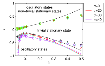
Figure 11: Phase diagram of the globally coupled two-delay network determined using the dichotomous model (solid lines) and numerical simulations of the Langevin model (markers). The phase diagram is show for different $\sigma=|\tau_{1}-\tau_{2}|/2$. The mean time delay is $\bar{\tau}=100$.

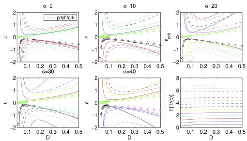
Figure 12: Upper panel and two lower left panels: Phase diagrams of our globally coupled two-delay network with $\bar{\tau}=100$ and $\sigma=0,\;10,\;20,\;30,\;40$. The green line depicts the critical coupling of the pitchfork bifurcation and the other lines depict those of the primary Hopf bifurcation as well as some higher order solutions (i.e. solutions 1-15) of Eq. 33 and 34. The markers depict the first bifurcation at $\varepsilon<0$ and $\varepsilon>0$ resulting from numerical simulations of the Langevin model (in these simulations, starting with $\varepsilon=0$, the coupling strength is increased until a bifurcation occurs). Matching colors of markers and lines mean that the bifurcation type and associated frequency are in agreement. Lower right panel: The frequencies of the corresponding unstable modes. They do not depend on $\sigma$, but slightly vary with the noise strength $D$.

IV Multiple delays

IV.1 Langevin model

In this Section we further generalize our delayed feedback system by introducing multiple time delays and study the stability properties in dependence of the statistical moments of an arbitrary time delay distribution.

The general Langevin model with many time delays reads

$$\dot{x}_{i}=x_{i}-x^{3}_{i}+\frac{\varepsilon}{N}\sum_{j=1}^{N}x_{j}(t-\tau_{ij})+\sqrt{2D}\xi(t).$$ (37)

Such general models in which the time delays depend on both the “transmitting” and the “receiving” element cannot directly be described in terms of a mean field theory. However, the system becomes mathematically tractable if we assume that the time delays only depend on the transmitting elements $j$,

$$\dot{x}_{i}=x_{i}-x^{3}_{i}+\frac{\varepsilon}{N}\sum\limits_{j=1}^{N}x_{j}(t-\tau_{j})+\sqrt{2D}\xi(t).$$ (38)

In order to check if such a simplification is justified, numerical simulations of model (37) and (38) are carried out and compared. In these simulations the distribution of the time delays is Gaussian, i.e., it is fully determined by its mean $\bar{\tau}$ and standard deviation $\sigma$. Fig. 13, comparing the critical coupling strength of the Hopf bifurcation for different $\sigma$, suggests that the above simplification is justified in order to study the stability properties of a bistable-element-network with time delays.

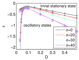
Figure 13: The critical coupling of the Hopf bifurcation as a function of the noise strength $D$ for different $\sigma$ of the Gaussian time delay distribution with $\bar{\tau=100}$. The markers and the solid lines depict the critical couplings resulting from model (37) and model (38), respectively.

This surprising result not only renders possible an analytical description of networks with distributed delays but also implies that the number of operations, which have to be carried out to study such systems numerically, can be reduced from ${\cal O}(N^{2})$ to ${\cal O}(N)$.

IV.2 Dichotomous theory

Let us now develop the dichotomous theory for the globally coupled bistable-element-network with distributed delays.

For that purpose we coarse grain system (38). The coarse graining is accomplished as follows: The range of possible time delays is divided up in $M$ intervals $I_{k}\;\{k=1,2,\ldots,M\}$. The size of the intervals $\Delta_{k}$ is chosen, so that the number of bistable oscillators associated with a delay, fitting in a particular interval, is for each interval the same $m=N/M$. In this way oscillator groups are formed whose mean field can be expressed as,

$$\Omega_{k}(t)\equiv\frac{1}{m}\sum_{\tau_{j}\in I_{k}}x_{j}(t),$$ (39)

where $I_{k}\equiv[\tau_{k},\tau_{k+1}[$, $\tau_{k}=\sum_{l=1}^{k-1}\Delta_{l}$ and $j=1\ldots N$.

Assuming that $\Delta_{k}\ll\bar{\tau}/\sigma$, where $\bar{\tau}$ and $\sigma$ are the mean and the standard deviation of the time delay distribution, Eq. (38) can then be approximated by,

$$x_{i}=x_{i}-x_{i}^{3}+\frac{\varepsilon}{M}\sum\limits_{k=1}^{M}\Omega_{k}(t-\tau_{k})+\sqrt{2D}\xi(t).$$ (40)

The master equations expressing the dynamics of system (40) in terms of occupation probabilities read,

$$\dot{n}_{1,k} = -p_{12}n_{1,k}+p_{21}n_{2,k}$$ (41)

$$\dot{n}_{2,k} = p_{12}n_{1,k}-p_{21}n_{2,k}.$$ (42)

Here the hopping probabilities are given by,

$$p_{12,21}=\frac{\sqrt{2\mp 3\alpha_{3}}}{2\pi}\exp\left(-\frac{1\mp 4\alpha_{3}}{4D}\right),$$ (43)

where $\alpha_{3}=(\varepsilon/M)\sum_{k=1}^{M}\Omega_{k}(t-\tau_{k})$.

For large oscillator groups $(m\to\infty)$, $\Omega_{k}=n_{1,k}s_{1}+n_{2,k}s_{2}=n_{2,k}-n_{1,k}$ holds. With this and the probability conservation $n_{1,k}+n_{2,k}=1$ we can find the following set of equations:

$$\dot{\Omega}_{k}(t)=p_{12}-p_{21}-(p_{21}+p_{12})\Omega_{k}(t).$$ (44)

The Jacobian matrix of this system is given through,

$$J=c\begin{pmatrix}g_{1}+d&g_{2}&\dots&g_{M}\\ g_{1}&g_{2}+d&\dots&g_{M}\\ {4}\\ g_{1}&g_{2}&\dots&g_{M}+d\\ \end{pmatrix},$$ (45)

where $c=-\sqrt{2}\exp(-1/4D)/(4M\pi D)$, $g_{k}=\varepsilon(3D-4)\exp(-\lambda\tau_{k})$ and $d=4MD$. With this Jacobian the characteristic equation, determining the stability of the trivial equilibrium $X=0$, becomes

$$(dc-\lambda)^{M-1}\left(c\left[d+\sum_{k=1}^{M}g_{k}\right]-\lambda\right)=0.$$ (46)

Setting $\lambda=0$ and solving Eq. (46) for $\varepsilon$ yields the critical coupling for the pitchfork instability,

$$\varepsilon_{\rm st}=\frac{4D}{4-3D}.$$ (47)

It is time delay independent and thus identical with that found in previous Sections of this paper.

The properties of the Hopf bifurcation (i.e. the frequencies of the unstable modes $\omega$ and the critical coupling $\varepsilon_{\rm osc}$ can be found by substituting $\lambda=\mu+{\rm i}\omega$ into Eq. (46), separating real and imaginary parts and setting $\mu=0$. This yields,

$$\omega\bar{\tau}=-\frac{\sqrt{2}}{\pi}\exp(-1/4D)\bar{\tau}\frac{I_{\rm s}}{I_{\rm c}},$$ (48)

where

$$I_{\rm s}=\frac{1}{M}\sum_{k=1}^{M}\sin\omega\tau_{k},\;\>I_{\rm c}=\frac{1}{M}\sum_{k=1}^{M}\cos\omega\tau_{k}.$$ (49)

For large systems $N\to\infty$, the number of groups $M\to\infty$ and thus

$$I_{s}=\int\limits_{0}^{\infty}P(\tau)\sin\omega\tau d\tau,\;\>I_{c}=\int\limits_{0}^{\infty}P(\tau)\cos\omega\tau d\tau,$$ (50)

where $P(\tau)$ is the time delay distribution function.

We can express the time delay distribution function in terms of cumulants $K_{n}$ (Van Kampen, 2003; Risken, 1989) and solve the integrals in (50):

$$I_{s}=\sin(g_{1})\exp({g_{2}}),\;\>I_{c}=\cos(g_{1})\exp({g_{2}}),$$ (51)

where

$$g_{1} = \sum_{m=0}^{\infty}\frac{({\rm i}\omega)^{2m+1}}{{\rm i}(2m+1)!}K_{2m+1},$$ (52)

$$g_{2} = \sum_{m=1}^{\infty}\frac{({\rm i}\omega)^{2m}}{(2m)!}K_{2m}.$$ (53)

Consequently,

$$\frac{I_{\rm s}}{I_{\rm c}}=\tan(g_{1}).$$ (54)

Since for symmetric distribution functions all odd cumulant moments except the first one $K_{1}=\bar{\tau}$ are zero, $I_{\rm s}/I_{\rm c}=\tan\omega\bar{\tau}$ holds. That is, in the case of a symmetric distribution of the time delays, the frequencies of the unstable modes in Eq. (48) depend only on the mean time delay.

Let us now determine the critical coupling of the Hopf bifurcation. For large time delays $\bar{\tau}\gg\tau_{K}$ the low-order solutions of the transcendental equation (48) yield frequencies $\omega\ll 1$. Thus the real part of equation (46) can be linearized near $\omega=0$ and the critical coupling of the Hopf bifurcation becomes,

$$\varepsilon_{\rm osc}=\frac{4D\pi\omega}{(3D-4)\left(\frac{1}{N}\sqrt{2}\exp(-1/4D)I_{\rm s}-\left[1-\frac{1}{N}\right]\pi\omega I_{\rm c}\right)}.$$ (55)

Then, for large systems $N\to\infty$ the critical coupling is,

$$\varepsilon_{\rm osc}=\frac{4D}{(4-3D)I_{\rm c}},$$ (56)

with $I_{\rm c}=3\sin(\omega\bar{\tau})\sin(5\omega\sigma/3)/(5\omega\sigma)$ and $I_{\rm c}=\cos(\omega\bar{\tau})\exp(-\omega^{2}\sigma^{2}/2)$ for uniform and Gaussian distributions, respectively.

IV.3 Phase diagrams

Eqs. (47), (48) and (56) are used to determine the phase diagram and the frequencies of the unstable oscillatory modes $f=\omega/(2\pi)$ of a bistable element network with uniformly distributed time delays . The theoretical predictions are compared with numerical simulations of the Langevin model (37). The number of bistable elements in these simulations is $N=300$. The results are shown in Figs. 14 and 15.

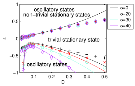
Figure 14: Phase diagram of the globally coupled bistable-element-network with uniformly distributed time delays derived from the theoretical model (solid lines) and numerical simulations of the Langevin model (markers). The phase diagram is shown for different standard deviations $\sigma$ of the delay distribution function. The mean time delay is $\bar{\tau}=100$.

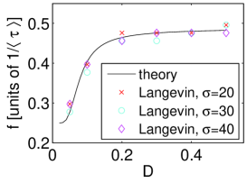
Figure 15: The frequencies of the unstable modes at the bifurcation points resulting from the Langevin model (markers) and the the dichotomous model (solid line), which are (see Eq. (48) independent of $\sigma$. For uniform and Gaussian distributions the frequencies depend only on the mean time delay (see Eq. 48 and 54).

Again, we find that near the transition points and for weak noise intensities the predictions of the dichotomous theory are reasonably good. Consequently, the Langevin models (37) and (38) are in this regime equivalent as regards the dynamical properties of the mean field.

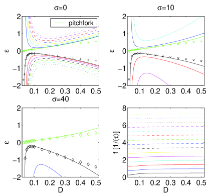
Figure 16: Same as in Fig. 12 but this time for networks with uniformly distributed time delays with $\tau=100$ and $\sigma=0,\>10,\>40$

Eqs. (48) and (56) have a multiplicity of solutions meaning that multistability is also present in our system in the limit of continuously distributed delays. The bifurcation diagrams including the higher order solutions are shown in Fig. 16. The Figure shows that unlike the two-delay system, the first transition at $\varepsilon<0$ is always determined by the primary solution associated with the frequency $f\approx 0.5\;\tau$.

The comparison of the phase diagrams for delay distribution functions of different widths $\sigma$ shows that the regions of oscillatory states in the parameter space are reduced with increasing $\sigma$. This trend was already apparent in the two-delay system, although less pronounced. These findings suggest that nonuniformity of the time delays inhibits the occurrence of Hopf bifurcations and consequently increases the stability of the trivial equilibrium.

Eventually, we like to mention that the coherence resonance phenomenon discussed in Sect. II.5 is also present in systems with multiple delays in the oscillatory domain of the phase diagram.

V Nonuniform coupling

V.1 Langevin model

The collective dynamics of the bistable-element-networks described above, is restricted to periodic oscillations and stationary states. In this Section we want to check whether the complexity of the dynamics is increased if instead of the uniform coupling, non-uniform couplings are applied. To this end, we extend the two time delay model (25) by introducing two different coupling strengths. The Langevin equations of the new model read,

$$\dot{x_{i}} =x_{i}-x_{i}^{3}+\frac{\epsilon_{1}}{2}X_{1}(t-\tau_{1})+\frac{\epsilon_{2}}{2}X_{2}(t-\tau_{2})+\sqrt{2D}\xi(t)$$ (57)

$$\dot{x_{j}} =x_{j}-x_{j}^{3}+\frac{\epsilon_{2}}{2}X_{1}(t-\tau_{1})+\frac{\epsilon_{1}}{2}X_{2}(t-\tau_{2})+\sqrt{2D}\xi(t),$$

where $i=1,\ldots,N/2$ and $j=N/2+1,\ldots,N$. The elements $x_{i}$ and $x_{j}$ belong to a group of bistable oscillators which are associated with time delay $\tau_{1}$ and $\tau_{2}$, respectively. It is assumed that the two groups are of equal size. The above set of equations describes a system in which each element couples to all the elements belonging to the same group with a coupling strength $\varepsilon_{1}$ and to all the elements of the other group with $\varepsilon_{2}$; that is, the two coupling parameters indicate the strength of the intra-group coupling $(\varepsilon_{1})$ and inter-group coupling $(\varepsilon_{2})$, respectively.

V.2 Dichotomous model

We apply the dichotomous theory to system (57) and proceed in a manner analogous to the previous sections.

The evolution of the mean field of each group of oscillators is described by

$$\dot{X}_{1,2}(t)=p^{1,2}_{12}-p^{1,2}_{21}-(p^{1,2}_{12}+p^{1,2}_{21})X_{1,2}(t).$$ (58)

Here, the hopping probabilities are,

$$p^{1}_{12,21} = \frac{\sqrt{2\mp 3\alpha_{4}}}{2\pi}\exp\left(-\frac{1\mp 4\alpha_{4}}{4D}\right),$$ (59)

$$p^{2}_{12,21} = \frac{\sqrt{2\mp 3\alpha_{5}}}{2\pi}\exp\left(-\frac{1\mp 4\alpha_{5}}{4D}\right),$$ (60)

where

$$\alpha_{4,5}=\left[\varepsilon_{1}X_{1,2}(t-\tau_{1})+\varepsilon_{2}X_{2,1}(t-\tau_{2})\right]/2.$$ (61)

Next a linear stability analysis is carried out. The linearization of Eq. 58 about the trivial equilibrium yields the Jacobian,

$$J=-c\begin{pmatrix}[3D-4]\varepsilon_{1}{\rm e}^{-\lambda\tau_{1}}+d&[3D-4]\varepsilon_{2}{\rm e}^{-\lambda\tau_{2}},\\ [3D-4]\varepsilon_{2}{\rm e}^{-\lambda\tau_{1}}&[3D-4]\varepsilon_{1}{\rm e}^{-\lambda\tau_{2}}+d\end{pmatrix},$$ (62)

where $c$ and $d$ are the same as in Eq. (31).

Substituting the trace $S$ and determinant $\Delta$ of the Jacobian matrix (62) into the characteristic equation

$$\lambda=\frac{S\pm\sqrt{S^{2}-4\Delta}}{2},$$ (63)

and keeping the intra-group coupling strength $\varepsilon_{1}$ fixed, yields the critical coupling for the pitchfork bifurcation, which can occur for positive and negative inter-group feedbacks,

$$\varepsilon^{\rm st}_{2}=\pm\left(\varepsilon_{1}+\frac{8D}{3D-4}\right).$$ (64)

In order to find the critical values for the Hopf bifurcation $\varepsilon^{\rm osc}_{2}$, we substitute $\lambda=\mu+{\rm i}\omega$ into the characteristic equation and set $\mu=0$. Then, the separation of real and imaginary part yields the two equations, $f_{\rm r}(\omega,\varepsilon_{2})=0$ and $f_{\rm i}(\omega,\varepsilon_{2})=0$, where

$$f_{\rm r}(\omega,\varepsilon_{2}) = E_{1}\varepsilon_{1}J_{s}\omega+\frac{E_{1}^{2}}{4}(\varepsilon^{2}_{1}-\varepsilon^{2}_{2})\cos(2\omega\bar{\tau})$$ (65)

$$+ E_{2}\varepsilon_{1}J_{c}+\frac{8}{\pi^{2}}\exp(-1/2D)-4\omega^{2},$$

$$f_{\rm i}(\omega,\varepsilon_{2}) = E_{1}\varepsilon_{1}J_{c}\omega+\frac{E_{1}^{2}}{4}(\varepsilon^{2}_{1}-\varepsilon^{2}_{2})\sin(2\omega\bar{\tau})$$ (66)

$$+ E_{2}\varepsilon_{1}J_{s}+\frac{8\sqrt{2}\omega}{\pi}\exp(-1/4D).$$

Here, $E_{1}=\sqrt{2}(3D-4)\exp(-1/4D)/(\pi D)$ and $E_{2}=E_{1}\sqrt{2}\exp(-1/4D)/\pi$. The terms $J_{s}$ and $J_{c}$ are given by Eq. (35) and (36), respectively.

For finite $\bar{\tau}$ and $\varepsilon_{2}$ the above set of equations has a finite number of roots $(\varepsilon^{\rm osc}_{2},\omega)$, which can be found numerically.

V.3 Phase diagram

In order to explore the dynamics of the system with two coupling strengths we carry out numerical simulations of the Langevin model (57) and compare the results with the theoretical predictions derived in the previous Section. In these simulations the strength of the intra-group coupling $\varepsilon_{1}$ and noise $D$ are chosen so that in the absence of inter-group couplings $\varepsilon_{2}=0$ the mean fields of the two oscillator groups $X_{1}$ and $X_{2}$ oscillate independently with frequencies $f_{1}\approx 1/2\tau_{1}$ and $f_{2}\approx 1/2\tau_{2}$ respectively (cf. Sect. II.3). We may then expect that for $|\varepsilon_{2}|>0$ the system reveals dynamical properties reminiscent of those of two coupled, limit-cycle oscillators, such as chaotic behavior (Woafo et al., 1996; Pastor et al., 1993; Matthews and Strogatz, 1990) and the amplitude death phenomenon (Atay, 2003; Herrero et al., 2000; Reddy et al., 1998). Fig. 17 shows time delay representations of the time series of $X_{1}(t)$ for inter-group couplings of different strength $\varepsilon_{2}$. In certain regions the system indeed shows the amplitude death phenomenon and in the range $0<|\varepsilon|<\varepsilon_{\rm chaos}$ irregular motions are observed. Numerical evidence suggests that these motions are chaotic. Indeed, the time series analysis yields broad band power spectra and positive maximum Lyapunov exponents. The determination of the Lyapunov exponents is below discussed in greater detail.

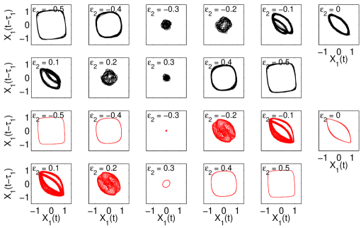
Figure 17: Time delay representations (phase portraits) of the evolution of the mean field $X_{1}$ in dependence of the inter-group coupling strength $\varepsilon_{2}$. Shown are the evolutions resulting from the Langevin model (upper two rows, Eq. 57) and the mean field model (lower two rows, Eq. 58). The parameters are: $D=0.1$, $\tau_{1}=60$, $\tau_{1}=140$, $\varepsilon_{1}=-0.4$.

The comparison of the phase portraits in Fig. 17 shows slight deviations between theoretical predictions and the Langevin dynamics (e.g. for $\varepsilon_{2}=-0.1$). These deviations stem from the elimination of the noise fluctuations in the dichotomous model and different phase shifts between the two oscillator groups $X_{1}$ and $X_{2}$. However, the predictive power of our model is confirmed in Fig. 18, where the theoretical peak power $P_{\rm peak}$ and the corresponding period $T_{\rm peak}$ in dependence of the coupling strength $\varepsilon_{1}$ are compared with those resulting from Langevin simulations.

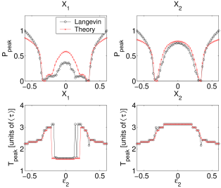
Figure 18: The peak power $P_{\rm peak}$ (upper row) and the corresponding period $T_{\rm peak}=2\pi/\omega_{\rm peak}$ (lower row) of the two oscillator groups $X_{1}$ and $X_{2}$ resulting from simulations of the theoretical mean field model (58) and the Langevin model (57), respectively. The parameters are the same as in Fig. 17.

Let us now explore the phase space of the system with nonuniform couplings in greater detail.

The phase space regions of nontrivial stationary states are determined by Eq. (64) and those where mean field oscillations and amplitude death occur, are given by the roots of Eq. (65) and (66). These roots are determined numerically. We find that the solutions of Eq. (33) are a subset of the the solutions of $f_{\rm r,i}(\omega)=0$. Thus, the corresponding critical values mark boundaries which qualitatively are equivalent to those found in previous models.

However, Eq. (65) also yields new solutions marking the boundaries between the the zones of amplitude death and the areas of nontrivial dynamics in the presence of weak inter-group couplings. Within this areas there may occur islands of chaotic dynamics. Indeed, an analysis of the mean field evolution yields positive Lyapunov exponents for $0<|\varepsilon|<\varepsilon_{\rm chaos}$.

Since intrinsically our time delay system is infinite dimensional the maximum Lyapunov exponents are here determined by an analysis of the time series resulting from Eq. (58). The analysis is carried out using tools provided by the TISEAN software package (Hegger et al., 1999; Kantz, 2004).

As stated above this process yields in some phase space regions clear evidence of positive maximum Lyapunov exponents in the range $0<\lambda\;[1/\bar{\tau}]\lesssim 0.03$.

The phase diagrams illustrating the different dynamic regions are shown in Fig. 19. The Figure shows that chaotic dynamics only occurs for strong intra-group couplings $\varepsilon_{1}\gtrsim 0.4$, i.e., when the individual oscillations of the two groups are strong enough.

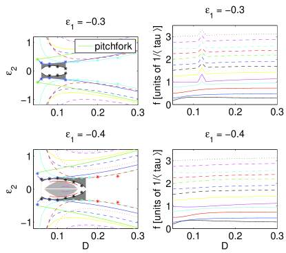
Figure 19: Same as in Fig. 12 but this time for a two time delay networks with nonuniform couplings (upper panels: $\varepsilon=-0.3$, lower panels: $\varepsilon=-0.4$). Oscillatory states as well as nontrivial stationary states occur for positive and negative inter-group couplings $\varepsilon_{2}$. Dark gray areas depict regions of amplitude death and the light gray areas mark regions of chaotic dynamics. The time delays are $\tau_{1}=60$ and $\tau_{2}=140$.

VI Summary and Conclusions

The dynamics of networks of noisy bistable elements with time-delayed couplings was studied analytically and numerically. Depending on the noise level, the systems undergo ordering transitions and demonstrate multistability; that is, for a strong enough positive feedback the systems adopt a nonzero stationary mean field state, and a variety of stable oscillatory mean field states are accessible for a positive as well as negative feedback. The coherence of the oscillatory states is maximal for a certain noise level; i.e., the systems demonstrate the coherence resonance phenomenon.

For symmetric time delay distributions the frequencies of the oscillations depend only on the mean time delay. However, the critical couplings of the corresponding Hopf bifurcations depend also on the higher order cumulants of the time delay distributions. Indeed, our findings suggest that nonuniformity of the time delays inhibits the occurrence of the Hopf bifurcations and consequently increases the stability of the trivial equilibrium. This may be important for time delay systems such as neural networks and genetic regulatory networks, since the degree of time delay nonuniformity, which is often related to the diversity in the connectivity of the underlying network, affects the accessibility of the nontrivial dynamical states.

The dichotomous theory based on delay-differential master-equations, which has been developed in this article, adequately describes the bifurcations of the trivial equilibrium in the limit of small noise and coupling strength. Furthermore, the theory allows for the application of a center manifold reduction and thus for a complete bifurcation analysis of the trivial equilibrium. Far away from the bifurcation points the mean field properties are well described by a Gaussian approximation. However, a theoretical approach for the description of the dynamics in the regime of strong noise near the transition points is still lacking.

The collective dynamics of the networks of bistable elements with uniform coupling strength is restricted to periodic oscillations and stationary states. However, our model with nonuniform coupling strengths shows that for certain coupling distributions, the system behaves like a network of coupled limit cycle oscillators and consequently, demonstrates in certain parameter-space areas the amplitude death phenomenon or exhibits a chaotic evolution of the mean field.

This paper discusses the dynamics of globally coupled systems with time delays. However, in many systems the connectivity is sparse. Since this is a particular case of systems with nonuniform coupling we may expect that this endows the system with more complex dynamical properties. This issue should be addressed in future studies.

References

- Dawson (1983) D. Dawson, J. Stat. Phys. 29, 31 (1983).
- Jung et al. (1992) P. Jung, U. Behn, E. Pantazelou, and F. Moss, Phys. Rev. A 46, R1709 (1992).
- Koulakov et al. (2002) A. Koulakov, S. Raghavachari, A. Kepecs, and J. Lisman, Nat. Neurosci. 5, 775 (2002).
- Camperi and Wang (1998) M. Camperi and X. Wang, J. Comp. Neurosci. 5, 383 (1998).
- Sompolinsky (1986) H. Sompolinsky, Phys. Rev. A 34, 2571 (1986).
- Gardner et al. (2000) T. Gardner, C. Cantor, and J. Collins, Nature 403, 339 (2000).
- Zanette (1997) D. H. Zanette, Phys. Rev. E 55, 5315 (1997).
- Reddy et al. (1998) D. Reddy, A. Sen, and G. Johnston, Phys. Rev. Lett. 80, 5109 (1998).
- Nakamura et al. (1994) Y. Nakamura, F. Tominaga, and T. Munakata, Phys. Rev. E 49, 4849 (1994).
- Bressloff and Coombes (1998) P. C. Bressloff and S. Coombes, Phys. Rev. Lett. 80, 4815 (1998).
- Choi and Huberman (1985) M. Y. Choi and B. A. Huberman, Phys. Rev. B 31, 2862 (1985).
- Wiesenfeld et al. (1990) K. Wiesenfeld, C. Bracikowski, G. James, and R. Roy, Phys. Rev. Lett. 65, 1749 (1990).
- Wiesenfeld and Hadley (1989) K. Wiesenfeld and P. Hadley, Phys. Rev. Lett. 62, 1335 (1989).
- Yeung and Strogatz (1999) M. K. S. Yeung and S. H. Strogatz, Phys. Rev. Lett. 82, 648 (1999).
- Van den Broeck and Parrondo (1994) C. Van den Broeck and J. Parrondo, Phys. Rev. E 49, 2639 (1994).
- Kuramoto (1991) Y. Kuramoto, Chemical Oscillations, Waves and Turbulence (Springer, Berlin, 1991).
- Shiino (1987) M. Shiino, Phys. Rev. A 36, 2393 (1987).
- Desai and Zwanzig (1978) R. C. Desai and R. Zwanzig, J. Stat. Phys. 19, 1 (1978).
- Tsimring and Pikovsky (2001) L. S. Tsimring and A. Pikovsky, Phys. Rev. Lett. 87, 250602 (2001).
- Huber and Tsimring (2003) D. Huber and L. S. Tsimring, Phys. Rev. Lett. 91, 260601 (2003).
- Salami et al. (2003) M. Salami, C. Itami, T. Tsumoto, and F. Kimura, PNAS 100, 6174 (2003).
- Paulsson and Ehrenberg (2001) J. Paulsson and M. Ehrenberg, Q. Rev. Biophys. 34, 1 (2001).
- Atay (2003) F. Atay, Phys. Rev. Lett. 91, 094101 (2003).
- Hänggi et al. (1990) P. Hänggi, P. Talkner, and M. Borkovec, Rev. Mod. Phys. 62, 251 (1990).
- Kramers (1940) H. Kramers, Physica (Utrecht) 7, 284 (1940).
- Pikovsky et al. (2002) A. Pikovsky, A. Zaikin, and M. A. de La Casa, Phys. Rev. Lett. 88, 050601 (2002).
- McNamara and Wiesenfeld (1989) B. McNamara and K. Wiesenfeld, Phys. Rev. A 39, 4854 (1989).
- Gammaitoni et al. (1998) L. Gammaitoni, P. Hänggi, P. Jung, and F. Marchesoni, Rev. Mod. Phys. 70, 223 (1998).
- Chow and Hale (1982) S. N. Chow and J. K. Hale, Methods of Bifurcation Theory (Springer, New York, 1982).
- Faria and Magalhães (1995) T. Faria and L. T. Magalhães, J . Diff. Eq. 122, 181 (1995).
- Giannakopoulos and Zapp (1999) F. Giannakopoulos and A. Zapp, J. Math. Anal. Appl. 237, 425 (1999).
- Redmond et al. (2002) B. F. Redmond, V. G. LeBlanc, and A. Longtin, Physica D 166, 131 (2002).
- Strogatz (2000) S. H. Strogatz, Nonlinear Dynamics and Chaos (Westview Press, Cambridge, 2000).
- Kiss et al. (2003) I. Z. Kiss, J. L. Hudson, G. J. Escalera Santos, and P. Parmananda, Phys. Rev. E 67, 035201 (2003).
- Miyakawa and Isikawa (2002) K. Miyakawa and H. Isikawa, Phys. Rev. E 66, 046204 (2002).
- Pikovsky and Kurths (1997) A. S. Pikovsky and J. Kurths, Phys. Rev. Lett. 78, 775 (1997).
- Sigeti and Horsthemke (1989) D. Sigeti and W. Horsthemke, J. Stat. Phys. 54, 1217 (1989).
- Zhou et al. (2001) C. Zhou, J. Kurths, and B. Hu, Phys. Rev. Lett. 87, 98101 (2001).
- Van Kampen (2003) N. Van Kampen, Stochastic Processes in Physics and Chemistry (Elesiver Scinece B.V., Amsterdam, The Netherlands, 2003).
- Risken (1989) H. Risken, The Fokker-Planck Equation (Springer, Berlin Heidelberg, 1989).
- Woafo et al. (1996) P. Woafo, J. C. Chedjou, and H. B. Fotsin, Phys. Rev. E 54, 5929 (1996).
- Pastor et al. (1993) I. Pastor, V. M. Pérez-García, F. Encinas, and J. M. Guerra, Phys. Rev. E 48, 171 (1993).
- Matthews and Strogatz (1990) P. C. Matthews and S. H. Strogatz, Phys. Rev. Lett. 65, 1701 (1990).
- Herrero et al. (2000) R. Herrero, M. Figueras, J. Rius, F. Pi, and G. Orriols, Phys. Rev. Lett. 84, 5312 (2000).
- Hegger et al. (1999) R. Hegger, H. Kantz, and T. Schreiber, Chaos 9, 413 (1999).
- Kantz (2004) H. Kantz, Nonlinear Time Series Analysis (Cambridge University Press, Cambridge, 2004).