Lineshape of harmonic generation by metal nanoparticles
and metallic photonic crystal slabs

Abstract

We study the linear and nonlinear-optical lineshapes of metal nanoparticles (theory) and metallic photonic crystal slabs (experiment and theory). For metal nanoparticle ensembles, we show analytically and numerically that femtosecond second- or third-harmonic-generation (THG) experiments together with linear extinction measurements generally do not allow to determine the homogeneous linewidth. This is in contrast to claims of previous work in which we identify a technical mistake. For metallic photonic crystal slabs, we introduce a simple classical model of two coupled Lorentz oscillators, corresponding to the plasmon and waveguide modes. This model describes very well the key experimental features of linear optics, particularly the Fano-like lineshapes. The derived nonlinear-optical THG spectra are shown to depend on the underlying source of the optical nonlinearity. We present corresponding THG experiments with metallic photonic crystal slabs. In contrast to previous work, we spectrally resolve the interferometric THG signal, and we additionally obtain a higher temporal resolution by using 5 fs laser pulses. In the THG spectra, the distinct spectral components exhibit strongly different behaviors versus time delay. The measured spectra agree well with the model calculations.
(Submitted to Phys. Rev. B on February 28, 2005; published in Phys. Rev. B 72, 115113 on September 15, 2005; resubmitted to arXiv on )
©2005 The American Physical Society

I Introduction

The linear-optical properties of metallic photonic crystal slabs (MPCSs) have recently attracted considerable attention because they can be viewed as a simple model system of two coupled oscillators: (i) a Lorentz oscillator electronic resonance couples to (ii) an electromagnetic resonance. (i) The electronic resonance comes about from charges which accumulate at the surface of the metal nanostructures when exposed to the electric field of the incident light. These charges induce a depolarization field that can either counteract or enhance the external electric field, depending on the permittivity of the metal, hence depending on the frequency of light. The resulting resonance at the transition point is the well-known particle plasmon or Mie resonance.KreibigBook (ii) The electromagnetic resonance is the Bragg resonance of the periodic arrangement with lattice constant $a$. Importantly, an appreciable coupling between these two oscillators requires an additional slab waveguide, e.g., underneath the metal nanoparticles. Therefore, the physics of metallic photonic crystal slabs is distinct from that of usual metallic gratings, which have been discussed extensively many years ago.NeviereBook Tailoring the waveguide parameters allows one to control the coupling strength, since the coupling arises from the spatial overlap of the plasmon- and waveguide-mode fields.

Two-dimensional MPCSs were first discussed in Ref. LindenPRL01, employing gold nanoparticles on a dielectric waveguide. Later,ChristPRL03 gold nanowires showed even more pronounced effects. In the latter structures, the coupling of the incident light to the particle plasmon resonance can conveniently be switched on and off via the polarization. If the electric field vector is oriented perpendicular to the nanowires (TM polarization), a pronounced depolarization field arises, giving rise to a strong optical resonance. In contrast, if the electric field vector is along the wire axis (TE polarization), the depolarization factor is zero and one rather gets a Drude-type response of the metal.

More recently, nonlinear-optical experiments on MPCSs have been presented.ZentgrafPRL04 These were interpreted along the lines of similar experimentsLamprechtAPB99 performed on metal nanoparticle ensembles on a substrate surface without a slab waveguide. Thus, our initial motivation was to continue with experiments along these lines and obtain additional information from nonlinear-optical experiments.

This paper contains both theory and experiments and is organized as follows. In Sec. II we start by discussing the nonlinear optics of metal nanoparticle ensembles with inhomogeneously broadened plasmon resonances. We derive rigorous analytic results for excitation with $\delta$ pulses and Lorentzian inhomogeneous broadening. Furthermore, we present numerical results for a Gaussian inhomogeneous broadening and finite-duration optical pulses. For second- (SHG) and third-harmonic generation (THG), we find that the interferometric nonlinear response exclusively depends on the total linear-optical linewidth of the particle plasmon, i.e., one cannot obtain any information on the relative contributions of homogeneous and inhomogeneous broadening, respectively. This finding is in striking disagreement with the claim of Ref. LamprechtAPB99, that interferometric SHG together with linear-optical measurements can differentiate between homogeneous and inhomogeneous broadening. Reference LamprechtAPB99, has been the basis of much if not most of the work that followed in this field.LamprechtPRL00 ; LamprechtPRL99 ; AusseneggPRB03 ; TraegerPRL00 ; TraegerAPB99 ; ZentgrafPRL04 ; WeidaJOSAB00 The discrepancy is traced back to a simple technical mistake in that work,LamprechtAPB99 where the authors have not properly differentiated between the contributions of second-harmonic generation on the one hand and optical rectification on the other hand. Indeed, optical rectification (OR), self-phase modulation (SPM), or four-wave mixing (FWM) would allow for such a differentiation. Next, in Sec. III, we discuss the linear-optical properties of two coupled oscillators (representing the particle plasmon and waveguide resonance). In contrast to frequent belief, the optical response of two coupled classical damped Lorentzian oscillators does not correspond to that of two new effective Lorentzian oscillators. Generally, one rather gets Fano-like lineshapes in the linear-optical spectra. In Sec. IV we discuss the nonlinear-optical signals from two coupled oscillators. We show that signatures of interferometric THG depend on the source of nonlinearity. Our theoretical analysis thus yields additional insights compared to the discussion in Ref. ZentgrafPRL04, . The parameters of the presented numerical calculations are chosen to allow for a direct comparison with our experimental results, which are presented in Sec. V. Compared with previous work, our experiments are distinct in two aspects, (a) and (b). (a) First, we use 5 fs optical pulses, which are within the range of the anticipated particle plasmon decay times of $0.7-9\,\rm fs$.FeldmannPRL02 Previous work used pulses of 13 fs duration and longer.LamprechtAPB99 ; ZentgrafPRL04 (b) As usual in “time-resolved spectroscopy,” indirect information on the temporal behavior is obtained by exciting the sample with a pair of time-delayed pulses, e.g., in pump-probe or transient four-wave mixing experiments. It is known that additional information can often be obtained by spectrally resolving the probe beam or the diffracted beam. In analogy, one anticipates that spectrally resolving the third-harmonic signal, generated by the sample, versus the time delay of two exciting pulses, gives additional insight. Indeed, our experiments reveal that different spectral components of the third-harmonic signal can exhibit substantially different temporal dynamics – information that would obviously not be available from a spectrally integrated experiment. The comparison of our experimental data with theory allows us to determine the dominant source of the underlying optical nonlinearity. Finally, we conclude in Sec. VI.

II Nonlinear optics of ensembles of Lorentzian oscillators

To probe metal nanoparticles with diameters in the 10–200 nm range by linear- or nonlinear-optical techniques, one often averages over several thousands of these particles in order to obtain an acceptable signal strength. Depending on the fabrication method (e.g., lithographic patterning,CraigheadAPL84 Volmer-Weber growth VolmerZPC26 ), a distribution in particle size and shape results, leading to a distribution of plasmon-resonance frequencies.KreibigBook Ensemble linear-optical experiments alone cannot distinguish this inhomogeneous contribution from the homogeneous linewidth (resulting from an expected plasmon decay time $\tau$ of a few femtoseconds). Therefore, e.g., a combination of linear and nonlinear methods has to be used to extract both homogeneous and inhomogeneous contributions. Nevertheless, not all nonlinear methods allow for this determination.

We begin by discussing analytic results for the limit of $\delta$ pulses and Lorentzian inhomogeneous broadening, and continue with numerical simulations for finite Gaussian inhomogeneous broadening and pulses of finite duration.

II.1 Analytic calculations

Following along the lines of Ref. LamprechtAPB99, , we start by describing the particle plasmon by an oscillating particle with charge $q$, mass $m$, and displacement $x(t)$, driven by an electric field $E(t)$ via

$$\ddot{x}+2\gamma\dot{x}+\Omega_{0}^{2}x+(\xi x^{2}+\eta x^{3}+...)=\frac{q}{m}E(t)\,.$$ (1)

For the interferometric experiments to be described, $E(t)$ corresponds to a pair of copropagating pulses with time delay $T$. In linear optics, i.e., for $\xi=\eta=...=0$, this leads to a Lorentz oscillator resonance at the damped eigenfrequency $\Omega=\sqrt{\Omega_{0}^{2}-\gamma^{2}}$ with a half width at half maximum (HWHM) $\gamma=1/T_{2}=1/(2\tau)$, the homogeneous linewidth. $T_{2}$ is the dephasing time. To first order in the laser electric field, the polarization $P^{(1)}\propto x^{(1)}(t)$ is given by

$$x^{(1)}(t)\propto\Omega^{-1}\,\int_{-\infty}^{t}dt^{\prime}\ \textrm{e}^{-\gamma(t-t^{\prime})}\ \sin[\Omega(t-t^{\prime})]\,E(t^{\prime})\,.$$ (2)

Upon excitation with resonant pulses, the Fourier transform of $P^{(1)}(t)$ contains frequency components around $\pm\Omega$. To second order in the laser electric field, $-\xi(x^{(1)}(t))^{2}$ is the driving term for the second-order displacement $x^{(2)}(t)$. Provided that this driving term is off-resonant with respect to $\Omega$, we obtain the second-order polarization $P^{(2)}(t)\propto x^{(2)}(t)$ with

$$x^{(2)}(t)\propto[x^{(1)}(t)]^{2}\,.$$ (3)

The Fourier transform of this expression contains frequency components around $\pm 2\Omega$, i.e., optical second-harmonic generation, and components around zero frequency, i.e., optical rectification. Furthermore, Ref. LamprechtAPB99, argued (see also formulae in Refs. LamprechtAPB97, ; TraegerAPB99, ) that the signal $S$ measured by a slow detector is given by the integral of the nonlinear intensity over time, i.e.,

$$S^{(2)}_{\rm SHG\,+\,OR}(T)\propto\int_{-\infty}^{\infty}dt\ [P^{(2)}(t)]^{2}\,.$$ (4)

It is crucial to note that this expression comprises both SHG and OR. This, however, is in contrast to what is actually measured in a second-order interferometric autocorrelation (IAC) setup, where one selectively detects the SHG by means of a photomultiplier tube behind optical filters, which suppress contributions other than SHG.remark

For reasons of simplicity and to allow for analytic results, we first discuss excitation with a pair of $\delta$ pulses, i.e.,

$$E(t)=\tilde{E}_{0}\,[\delta(t)+\delta(t-T)]\,.$$ (5)

It is clear from the symmetry that the nonlinear signals only depend on $|T|$. Thus, we only consider $T\geq 0$ in what follows. For a single homogeneously broadened oscillator we obtain

$$P^{(1)}(t) \propto \Omega^{-1}\{\Theta(t)\,\textrm{e}^{-\gamma t}\sin(\Omega t)$$ (6)

$$+\Theta(t-T)\,\textrm{e}^{-\gamma(t-T)}\sin[\Omega(t-T)]\}\,.$$

This leads to the second-order polarization

$$P^{(2)}(t)$$

$$\propto \Omega^{-2}(\Theta(t)\,\textrm{e}^{-2\gamma t}[1-\cos(2\Omega t)]$$

$$+\Theta(t-T)\,\textrm{e}^{-2\gamma(t-T)}\{1-\cos[2\Omega(t-T)]\}$$

$$+2\Theta(t-T)\,\textrm{e}^{-\gamma(2t-T)}\{\cos(\Omega T)-\cos[\Omega(2t-T)]\})\,.$$

Let us now consider an inhomogeneously broadened ensemble of oscillators with fixed damping $\gamma$ and a Lorentzian distribution of eigenfrequencies $\Omega$ with distribution function

$$\rho(\Omega)=\frac{\Gamma/\pi}{(\Omega-\overline{\Omega})^{2}+\Gamma^{2}}\,,$$ (8)

which is centered around frequency $\overline{\Omega}$. The HWHM of this inhomogeneous distribution is $\Gamma$. To work out the convolution, we approximate the prefactor $1/\Omega^{2}$ in Eq. (II.1) by $1/\overline{\Omega}^{2}$. This approximation is justified in the limit $\Gamma\ll\overline{\Omega}$, which is usually well satisfied for lithographically fabricated particles. These two steps together lead to

$$P^{(2)}_{\rm inhom}(t) \propto \int_{-\infty}^{\infty}d\Omega\,\rho(\Omega)P^{(2)}(t)$$

$$\propto +\Theta(t)\,\textrm{e}^{-2\gamma t}$$

$$+\Theta(t-T)\,\textrm{e}^{-2\gamma(t-T)}$$

$$+2\Theta(t-T)\,\textrm{e}^{-\gamma(2t-T)-\Gamma T}\cos(\overline{\Omega}T)$$

$$-\Theta(t)\,\textrm{e}^{-2(\gamma+\Gamma)t}\cos(2\overline{\Omega}t)$$

$$-\Theta(t-T)\,\textrm{e}^{-2(\gamma+\Gamma)(t-T)}\cos[2\overline{\Omega}(t-T)]$$

$$-2\Theta(t-T)\,\textrm{e}^{-(\gamma+\Gamma)(2t-T)}\cos[\overline{\Omega}(2t-T)]\,.$$

The first three lines correspond to OR, the last three lines to SHG. Note that the latter solely depends on the total width $\gamma+\Gamma$. In linear optics, the width of the inhomogeneous ensemble results from the convolution of a Lorentzian with homogeneous width $\gamma$ with a Lorentzian of inhomogeneous width $\Gamma$. This leads to a total width of the resonance in linear optics of $\gamma+\Gamma$. Thus, both the linear response and the correctly calculated SHG depend in the very same manner on the homogeneous and inhomogeneous linewidth, and a distinction is strictly not possible.

In contrast, the contribution from OR does not simply depend on $\gamma+\Gamma$, potentially allowing for a distinction between homogeneous and inhomogeneous linewidths. By erroneously including OR in the calculated interferometric “SHG signal,” one can seemingly separate the homogeneous and inhomogeneous contributions to the linewidth.

We have performed an analogous calculation for the third-order nonlinear-optical response. For third-harmonic generation and $T\geq 0$, we find that the ensemble THG polarization is

$$P^{(3)}_{\rm THG,\,inhom}(t)$$ (10)

$$\propto -\Theta(t)\,\textrm{e}^{-3(\gamma+\Gamma)t}\cos(3\overline{\Omega}t)$$

$$-\Theta(t-T)\,\textrm{e}^{-3(\gamma+\Gamma)(t-T)}\cos[3\overline{\Omega}(t-T)]$$

$$-3\Theta(t-T)\,\textrm{e}^{-(\gamma+\Gamma)(3t-T)}\cos[\overline{\Omega}(3t-T)]$$

$$-3\Theta(t-T)\,\textrm{e}^{-(\gamma+\Gamma)(3t-2T)}\cos[\overline{\Omega}(3t-2T)]\,.$$

The THG again only depends on $\gamma+\Gamma$, and no information on the homogeneous linewidth $\gamma$ can be obtained. However, self-phase modulation would provide such information. In a non-copropagating geometry, the latter would give rise to a diffracted four-wave-mixing signal. Corresponding calculations have been presented in Ref. WegenerPRA90, .

Broadly speaking, nonlinear-optical signals of the type $\omega+\omega$ (SHG) or $\omega+\omega+\omega$ (THG), etc. do not allow one to distinguish between homogeneous and inhomogeneous contributions to the linewidth, whereas signals of the type $\omega-\omega$ (OR) or $\omega+\omega-\omega$ (SPM or FWM), etc. do allow for such distinction. The “-” sign in OR, SPM, FWM, etc., effectively reverses the time axis in analogy to phase conjugation. For example in FWM, the “-” sign leads to the well-known photon-echo response.WegenerPRA90 At this point, a decay of the ensemble polarization due to inhomogeneous broadening (just interference) can be reversed, whereas damping due to homogeneous broadening (a dissipative process) cannot be reversed.

II.2 Numerical calculations

The presented analytical calculations for $\delta$ pulses are appropriate if the (complex) laser electric field spectrum exhibits negligible variation on the scale of the homogeneous linewidth $\gamma$. For longer pulses, we have performed numerical simulations. As described above, the correct way to calculate the SHG contribution is to spectrally filter the second-order response of the oscillator ensemble. To obtain the final IAC signal as a function of the time delay $T$, the square modulus of this filtered second-order polarization has to be integrated with respect to frequency. To allow for a direct comparison with the results of Ref. LamprechtAPB99, , we also use sech²-shaped 15 fs pulses with a center wavelength of 780 nm, resonantly exciting the ensemble. The latter has a Gaussian distribution of resonances and is discretized in steps of 1 nm.

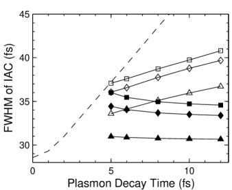
Figure 1: Recalculated data of Fig. 2 of Ref. LamprechtAPB99, . The dashed line describes the simulated FWHM of the second-order interferometric autocorrelation (IAC) from a single resonant Lorentz oscillator (the particle plasmon) versus plasmon decay time $\tau=T_{2}/2$. The solid lines represent ensembles of oscillators with eigenfrequencies following a Gaussian distribution, for which the width is determined by fixing the total extinction linewidth $\Delta\lambda$ (squares, $\Delta\lambda$=70 nm; diamonds, $\Delta\lambda$=80 nm; triangles, $\Delta\lambda$=125 nm). The autocorrelation width is indicated by the full symbols for considering only the contribution of SHG. Corresponding results for (erroneously) including SHG and OR are shown by the open symbols.

Figure 1 shows the resulting full width at half maximum (FWHM) of the interferometric autocorrelation as a function of the plasmon decay time $\tau$. The full symbols correspond to the correct calculation, whereas the open symbols erroneously comprise the OR contribution and qualitatively reproduce the results of Ref. LamprechtAPB99, (see their Fig. 2). For each of the curves in our Fig. 1, the total linewidth of the linear-optical spectrum is fixed. The squares, diamonds, and triangles correspond to a fixed extinction linewidth (FWHM) of $\Delta\lambda=70$, $80$, and $125\,\rm nm$, respectively (see parameters of Fig. 2 of Ref. LamprechtAPB99, ). The dashed curve corresponds to a single (homogeneously broadened) oscillator for reference. The correct results and those including the OR contribution differ strongly – as in our analytical calculations. In particular, the slopes of the correct curves in our Fig. 1 are very nearly zero (within typical experimental error bars of 1 fs), while the incorrect simulations have a small positive slope. Thus, using the correct curves one cannot infer the plasmon decay time from measured interferometric autocorrelations, whereas the incorrect curves erroneously suggest this possibility.LamprechtAPB99 We conclude that, under inhomogeneous conditions, the homogeneous linewidth cannot be determined by analyzing linewidths from linear optics and SHG (or THG) measurements. Consequently, we will refrain from making any quantitative statements about plasmon decay times from now on.

We note in passing that the IAC acquires artificial “wings” LamprechtAPB99 if the OR contribution is erroneously included. Indeed, such wings are visible in Fig. 1a of Ref. LamprechtAPB99, . They disappear in the correct calculation (not shown).

III Linear optics of two coupled Lorentzian oscillators

In this section, we discuss the linear-optical properties of two coupled Lorentz oscillators. As already mentioned in the introduction, this system can serve as a simple model for metallic photonic crystal slabs. The results of this Sec. can be compared with the linear-optical experiments (Sec. V) and, furthermore, are the basis for our discussion of the nonlinear-optical properties in Sec. IV.

Generalizing Eq. (1) to two coupled, oscillating particles of equal mass $m$ leads to

$$\ddot{x}_{\rm pl}\!+\!2\gamma_{\rm pl}\dot{x}_{\rm pl}\!+\!\Omega_{\rm pl}^{2}x_{\rm pl}\!+\!({\rm NL})_{\rm pl}\!-\!\Omega_{\rm c}^{2}x_{\rm wg} = \frac{q_{\rm pl}}{m}E(t)\,,$$

$$\ddot{x}_{\rm wg}\!+\!2\gamma_{\rm wg}\dot{x}_{\rm wg}\!+\!\Omega_{\rm wg}^{2}x_{\rm wg}\!+\!({\rm NL})_{\rm wg}\!-\!\Omega_{\rm c}^{2}x_{\rm pl} = \frac{q_{\rm wg}}{m}E(t)\,.$$

Here, $x_{\rm pl}(t)$ and $x_{\rm wg}(t)$ are the displacements representing the plasmon and waveguide oscillations, respectively. The resonance frequencies, (homogeneous) half widths at half maximum, and oscillator strengths of the uncoupled system are denoted by $\Omega_{j}$, $\gamma_{j}$, and $q_{j}$ (${j}={\rm pl,wg}$), respectively. $\Omega_{\rm c}^{2}$ represents the coupling strength between the oscillators. The nonlinear terms (denoted by $\rm NL$) are discussed in Sec. IV and ignored here.

In order to make the resulting formulas transparent, we immediately discuss a few parameters in terms of their experimentally relevant values. Since the uncoupled waveguide resonance is extremely sharp SharonJOSAA97 as compared to the plasmon width, we set the waveguide damping $\gamma_{\rm wg}=0$. In the following, we derive formulas for an arbitrary waveguide oscillator strength $q_{\rm wg}$; however, most aspects can already be understood in the simpler case $q_{\rm wg}=0$. For typical sample parameters, $|q_{\rm wg}|\ll|q_{\rm pl}|$, i.e., the area under the extinction curve of the (uncoupled) waveguide mode is much smaller than that of the plasmon.

In the frequency domain, Eqs. (11) can easily be solved analytically. For monochromatic excitation, i.e., for $E(t)=\tilde{E}_{0}\,e^{-i\omega t}+{\rm c.c.}$, this leads to the first-order displacements $x^{(1)}_{j}(t)=\tilde{x}^{(1)}_{j}(\omega)\,e^{-i\omega t}+{\rm c.c.}$ and the polarizations $\tilde{P}^{(1)}_{j}(\omega)=N\,q_{j}\,\tilde{x}^{(1)}_{j}(\omega)$. $N$ is the density of the oscillators. Note that in the case $q_{\rm wg}=0$, only $\tilde{x}^{(1)}_{\rm pl}(\omega)$ contributes to the polarization. The total linear polarization becomes

$$\tilde{P}^{(1)}(\omega)=\frac{N}{m}\,\frac{q_{\rm pl}^{2}(-\omega^{2}+\Omega_{\rm wg}^{2})+2q_{\rm pl}q_{\rm wg}\Omega_{\rm c}^{2}+q_{\rm wg}^{2}(-\omega^{2}-2i\omega\gamma_{\rm pl}+\Omega_{\rm pl}^{2})}{(-\omega^{2}-2i\omega\gamma_{\rm pl}+\Omega_{\rm pl}^{2})(-\omega^{2}+\Omega_{\rm wg}^{2})-\Omega_{\rm c}^{4}}\,\tilde{E}_{0}\,.$$ (12)

The linear susceptibility $\tilde{\chi}^{(1)}(\omega)=\tilde{P}^{(1)}(\omega)/(\varepsilon_{0}\tilde{E}_{0})$ and the absorption coefficient

$$\alpha(\omega)=(\omega/c_{0})\,\mathrm{Im}[\tilde{\chi}^{(1)}(\omega)]=\alpha_{\rm pl}\,\frac{4\gamma_{\rm pl}^{2}\omega^{2}[\omega^{2}-\Omega_{\rm wg}^{2}-(q_{\rm wg}/q_{\rm pl})\Omega_{\rm c}^{2}]^{2}}{[(\omega^{2}-\Omega_{\rm pl}^{2})(\omega^{2}-\Omega_{\rm wg}^{2})-\Omega_{\rm c}^{4}]^{2}\,+\,4\gamma_{\rm pl}^{2}\omega^{2}(\omega^{2}-\Omega_{\rm wg}^{2})^{2}}$$ (13)

immediately follow. $\varepsilon_{0}$ is the vacuum permittivity, $c_{0}$ the vacuum speed of light, and $\alpha_{\rm pl}=Nq_{\rm pl}^{2}/(2m\varepsilon_{0}c_{0}\gamma_{\rm pl})$ the maximum absorption coefficient of the uncoupled plasmon oscillation.

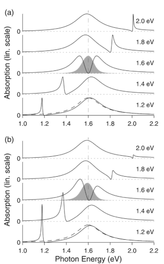
Figure 2: Optical absorption spectra according to Eq. (13) (solid lines). One observes an anticrossing behavior when varying the waveguide resonance frequency $\Omega_{\rm wg}$ with respect to the fixed plasmon resonance frequency $\Omega_{\rm pl}$. Note the highly asymmetric, Fano-like lineshape of the peaks. All curves are displayed on the same scale. $q_{\rm wg}/q_{\rm pl}$ equals 0 in (a) and $+0.1$ in (b). Common parameters are $\hbar\Omega_{\rm pl}=1.6\,\rm eV$, $\hbar\Omega_{\rm wg}$ as denoted for each curve, $\gamma_{\rm pl}=1/(2\tau)$, $\tau=2.5\,\rm fs$, and $\hbar\Omega_{\rm c}=0.5\,\rm eV$. The dashed lines represent the pure plasmonic absorption in the absence of coupling, i.e., for $\hbar\Omega_{\rm c}=0$. The gray areas shown for $\Omega_{\rm wg}=1.6\,\rm eV$ depict the square modulus of the waveguide amplitude, $|\tilde{x}^{(1)}_{\rm wg}|^{2}$, each exhibiting a single peak. In (a), the square modulus of the plasmon amplitude, $|\tilde{x}^{(1)}_{\rm pl}|^{2}$, is roughly proportional to the corresponding absorption spectrum. The vertical line is a guide to the eye.

Examples of absorption spectra are shown in Fig. 2(a) for $q_{\rm wg}/q_{\rm pl}=0$ and Fig. 2(b) for $q_{\rm wg}/q_{\rm pl}=+0.1$. One obtains the anticipated anticrossing behavior. For $q_{\rm wg}=0$, absorption maxima appear at the spectral positions

$$\Omega_{\rm a,b}^{2}=\left(\Omega_{\rm pl}^{2}+\Omega_{\rm wg}^{2}\right)/2\ \pm\ \left[\left(\Omega_{\rm pl}^{2}-\Omega_{\rm wg}^{2}\right)^{2}/4+\Omega_{\rm c}^{4}\right]^{1/2}\,.$$ (14)

These positions coincide with the normal mode frequencies of the coupled, but undamped system. For small $\Omega_{\rm c}$ and for $\Omega_{\rm pl}=\Omega_{\rm wg}$, the corresponding Rabi splitting is given by $\Omega_{\rm c}^{2}/\Omega_{\rm pl}$. Hence, the two oscillators can be considered as “resonant” if $|\Omega_{\rm pl}-\Omega_{\rm wg}|\ll\Omega_{\rm c}^{2}/\widehat{\Omega}$ with $\widehat{\Omega}=(\Omega_{\rm pl}+\Omega_{\rm wg})/2$, and as “nonresonant” otherwise. In contrast to frequent belief, the lineshapes in Fig. 2 do not correspond to the sum of two effective Lorentz oscillators. One rather gets a highly asymmetric, Fano-like lineshape. Usually, a Fano resonance results from the coherent interaction of a discrete quantum mechanical state with a continuum of states.FanoPR61 ; Marburg In our purely classical model, a single sharp oscillator coherently interacts with a strongly broadened second oscillator. The latter replaces the continuum. One result of the Fano-like interaction is that one obtains zero absorption between the two absorption maxima. The position of this zero appears at the root of the numerator of (13), i.e., at or near the spectral position of the (uncoupled) waveguide mode $\Omega_{\rm wg}$. Intuitively, this minimum is a result of destructive interference, which effectively suppresses the response of the two absorption “channels,” of which the polarizations have a phase difference near $\pi$. This phase difference will also be important in nonlinear optics (see Sec. IV). When $q_{\rm wg}$ is changed from zero to a nonzero value, the positions of the absorption extrema shift slightly, and the two peaks exhibit different heights as an additional characteristic. A reduced absorption of the more waveguide-like channel results, e.g., in the case $q_{\rm wg}/q_{\rm pl}>0$ and $\Omega_{\rm pl}<\Omega_{\rm wg}$ [see top curves in Fig. 2(b)].

We note that, e.g., for $q_{\rm wg}=0$, the total absorption (13) can be rewritten as a sum of two “Lorentzians,” but with strongly frequency-dependent dampings. In the time domain, these frequency-dependent dampings correspond to a non-Markovian (and non-exponential) decay. For $\Omega_{\rm a}<\Omega_{\rm wg}<\Omega_{\rm b}$, one solution can be described by oscillator a with constant resonance frequency $\Omega_{\rm a}$ and frequency-dependent damping

$$\gamma_{\rm a}(\omega)$$

$$= \left\{\begin{array}[]{r@{,\ \ }l}\frac{\gamma_{\rm pl}\alpha_{\rm pl}}{2\alpha(\omega)}\left(1+\left[1-\frac{\alpha^{2}(\omega)\left(\omega^{2}-\Omega_{\rm a}^{2}\right)^{2}}{\alpha_{\rm pl}^{2}\gamma_{\rm pl}^{2}\omega^{2}}\right]^{1/2}\right)&\omega<\Omega_{\rm wg}\\ \infty&\omega\geq\Omega_{\rm wg}\\ \end{array}\right.$$ (17)

and an analogous expression for the oscillator b.

IV Nonlinear optics of two coupled Lorentzian oscillators

In this section, we discuss the nonlinear-optical properties of two coupled Lorentz oscillators in terms of third-harmonic generation. We consider an inversion-symmetric medium, hence all second-order nonlinear terms in Eqs. (11) are zero. At first sight, one might only expect third-order nonlinear terms like $({\rm NL})_{\rm pl}\propto x_{\rm pl}^{3}$ or $({\rm NL})_{\rm wg}\propto x_{\rm wg}^{3}$ in Eqs. (11). Mathematically, the most general form is given by the terms

$$\eta_{j,k}[x_{\rm pl}(t)]^{3-k}[x_{\rm wg}(t)]^{k}$$ (19)

appearing in the differential equation for $x_{j}(t)$, respectively (${j}={\rm pl,wg};k=0,1,2,3$). Here, we are only interested in THG, which is off-resonant. In a perturbational approach the THG contributions to the third-order displacements are given by

$$x^{(3)}_{j}(t)\propto\sum_{k=0}^{3}\eta_{j,k}[x^{(1)}_{\rm pl}(t)]^{3-k}[x^{(1)}_{\rm wg}(t)]^{k}\,.$$ (20)

The eight parameters $\eta_{j,k}$ can be reduced to four, i.e., $\eta_{k}=\sum_{j}q_{j}\eta_{j,k}$ with $k=0,1,2,3$, because the optical polarization is given by the weighted sum of the displacements. This immediately leads to the following general form for the THG contribution to the third-order polarization

$$P^{(3)}(t)\propto\sum_{k=0}^{3}\eta_{k}[x^{(1)}_{\rm pl}(t)]^{3-k}[x^{(1)}_{\rm wg}(t)]^{k}\,.$$ (21)

We note in passing that this form is generally different from the ansatz $P^{(3)}(t)\propto[P^{(1)}(t)]^{3}$ (in analogy to Ref. ZentgrafPRL04, ), which leads to $\eta_{k}\propto{3\choose k}\,q_{\rm pl}^{3-k}q_{\rm wg}^{k}$.

For the numerical computation of THG spectra, we start off in the time domain. $E(t)$ is chosen OurPulses to resemble the 5 fs laser pulses of the experiments (5 fs Gaussian pulses deliver qualitatively similar results for all conditions discussed below). Furthermore, we fix $\Omega_{\rm pl}=1.67\,\rm eV$, $\Omega_{\rm wg}=1.56\,\rm eV$, $\Omega_{\rm c}=0.66\,\rm eV$, $\tau=1.06\,\rm fs$, and $q_{\rm wg}/q_{\rm pl}=+0.085$. These parameters correspond to sample A in Sec. V, which can be considered as “resonant” according to the definition given in Sec. III. Integration of Eqs. (11) yields the first-order displacements $x^{(1)}_{j}(t)$ and, with (21), the third-order polarization. The square modulus of its filtered Fourier transform delivers the THG intensity spectrum. Spectra are calculated as a function of the spectrometer photon energy and the time delay between the two excitation pulses, $T$.

We first discuss the case $\eta_{k}\propto\delta_{k,0}$ ($\delta_{k,l}$ is the Kronecker symbol). The corresponding data set is shown in Fig. 3(a). A cut at $T=0$ (not shown) reveals four broad but clearly distinct spectral peaks in the THG spectrum. The appearance of four peaks can easily be understood in the frequency domain, since the third-order polarization for this case is proportional to the twofold convolution of the displacement $\tilde{x}^{(1)}_{\rm pl}(\omega)$ with itself, this displacement containing two peaks [see, e.g., Fig. 2(a)]. The relative weights of the four peaks can be estimated employing the time domain. Assuming $\delta$ pulses, $q_{\rm wg}=0$, and neglecting damping, the two effective oscillators (see previous section) have comparable amplitude, and the general form of the THG polarization is proportional to    

$$[\cos(\Omega_{\rm a}t)+\cos(\Omega_{\rm b}t)]^{3} \propto ...$$ (22)

$$+\cos(3\Omega_{\rm a}t)$$

$$+3\cos[(2\Omega_{\rm a}+\Omega_{\rm b})t]$$

$$+3\cos[(\Omega_{\rm a}+2\Omega_{\rm b})t]$$

$$+\cos(3\Omega_{\rm b}t)\,.$$

This contains terms at three times the normal mode frequencies $\Omega_{\rm a}$ and $\Omega_{\rm b}$ as well as spectral mixing products. The relative amplitudes 1:3:3:1 of the frequency components $3\Omega_{\rm a}$, $2\Omega_{\rm a}+\Omega_{\rm b}$, $\Omega_{\rm a}+2\Omega_{\rm b}$, and $3\Omega_{\rm b}$ lead to the intensity ratios 1:9:9:1. This means that the two central frequency components are more prominent, in agreement with the numerical findings in Fig. 3(a).

The pronounced dips between the four spectral peaks are closely related to the Fano-like lineshapes discussed in Sec. III. In linear optics, the phase relation between the two effective oscillators (absorption “channels”) leads to destructive interference, and hence to zero absorption in the dip. The same destructive interference is also responsible for the deep dips in the THG spectra.

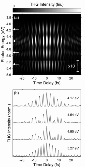
Figure 3: (a) Optical THG intensity derived from the coupled nonlinear oscillators. The THG intensity is shown on a saturated gray scale, versus spectrometer photon energy and time delay $T$ between the two excitation pulses. At $T=0$, the THG spectrum exhibits four distinct peaks (the high-energy peak is amplified by a factor of 10 for the sake of clarity). The four peaks exhibit different temporal behaviors. Corresponding cuts at the spectral peak positions indicated by the white arrows in (a) are shown in (b). For better comparison, the curves are normalized to the same maximum and are vertically displaced. Obviously, the first and fourth curves both have a smoothly decaying (upper) envelope, while only the second and third curves show an envelope resulting from a beating. The nonlinearity parameters used are $\eta_{k}\propto\delta_{k,0}$. The other parameters are quoted in the text. Compare with the corresponding experiment (Fig. 8 below).

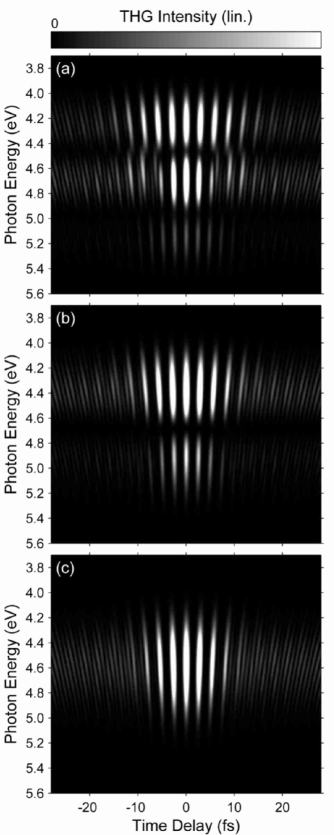
Figure 4: As Fig. 3(a), but for different nonlinearity parameters. The shown THG contributions result from a nonzero value of (a) $\eta_{1}$, (b) $\eta_{2}$, and (c) $\eta_{3}$ while keeping the other nonlinearity parameters zero. At $T=0$, the number of spectral peaks is three, two, and one, respectively. (a), (b), and (c) are displayed on individual gray scales.

The behavior of the THG intensity as a function of time delay $T$ differs among the four spectral peaks. Corresponding cuts at the spectral peak positions indicated by the white arrows in Fig. 3(a) are shown in Fig. 3(b). The curves exhibit the usual oscillations with the respective fundamental and harmonic frequencies, enclosed in the (upper) envelope of interest. The first and fourth curves clearly show a smoothly decaying envelope for increasing $|T|$. In contrast, the envelopes of the central two curves (which are associated with the spectral mixing products) reveal a beating. In spectrally integrated measurements,ZentgrafPRL04 this distinction is not possible.

So far, we have only discussed the case $\eta_{k}\propto\delta_{k,0}$. Next, we calculate corresponding THG spectra for different nonlinearity parameters (Fig. 4). In each part of this figure, all nonlinear parameters are zero except for a single one. The parts (a), (b), and (c) result from a nonzero value of $\eta_{1}$, $\eta_{2}$, and $\eta_{3}$, showing three peaks, two peaks, and one peak, respectively. In the frequency domain this can again be understood by the corresponding convolutions. Remember that $\tilde{x}^{(1)}_{\rm pl}(\omega)$ contains two peaks for the values chosen here, whereas $\tilde{x}^{(1)}_{\rm wg}(\omega)$ only contains one peak (refer to gray areas in Fig. 2).

In general, all parameters $\eta_{k}$ can have nonzero values simultaneously. When adding up the nonlinear contributions to the polarization, interference can result in a THG intensity with amplified or suppressed spectral peaks and dips, spectrally shifted peak positions, or even with new peaks or dips which are not present at all in Figs. 3(a) and 4. We will not go into a detailed analysis. We only note that for $\eta_{0}\gg\eta_{1}>\eta_{2}=\eta_{3}=0$, the tendency is to suppress the high-energy peaks compared to the case $\eta_{0}\neq 0$ and $\eta_{1}=\eta_{2}=\eta_{3}=0$.

The key feature of the calculations presented so far is that the THG spectra depend on the underlying source of the nonlinearity, i.e., they depend on which of the coefficients $\eta_{k}$ is nonzero. In other words, observing four, three, two, or just one peak in experimental THG spectra allows one to learn something about the system by comparison with theory. This, however, is only possible for a certain regime of coupling between the two oscillators, which we shall refer to as the regime of “moderate coupling.” Obviously, for very small coupling strengths, i.e., for small values of $\Omega_{\rm c}$, the four spectral peaks in the THG spectrum of the case $\eta_{k}=\delta_{k,0}$ (discussed above) merge into a single peak. In the other limit, i.e., for large values of $\Omega_{\rm c}$, also $\tilde{x}^{(1)}_{\rm wg}(\omega)$ exhibits several peaks (unlike the gray areas in Fig. 2), which can, for example, lead to several spectral peaks in the THG spectrum for the case $\eta_{k}=\delta_{k,3}$ as well. By numerical calculations for the “resonant” case (i.e., $\Omega_{\rm pl}=\Omega_{\rm wg}=\widehat{\Omega}$), for $q_{\rm wg}=0$, and assuming $\delta$ pulses, we can specify the regime of “moderate coupling” by the condition $0.15<\Omega_{c}^{2}/(2\gamma\widehat{\Omega})<1.35$. Thus, if one wants to learn something from the comparison of experiment and theory, the coupling parameter of a sample has to be tailored correspondingly.

V Experiments

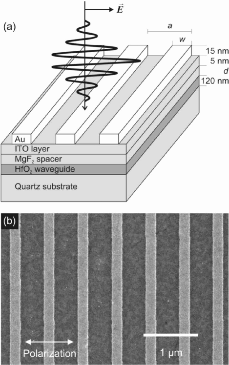
Figure 5: (a) Scheme showing gold nanowires on top of a set of dielectric layers forming the slab waveguide. HfO₂ is used as a high-index material, while MgF₂ serves as a low-index spacer. The polarization of the normally incident white light or laser pulses is perpendicular to the wires (TM polarization) for the experiments shown in Figs. 6, 8, and 9. Samples with different lattice constant $a$, wire width $w$, and spacer thickness $d$ are investigated. (b) Scanning electron micrograph of the gold nanowires (light gray) on top of the waveguide (dark gray).

The system of interest, a metallic photonic crystal slab, is schematically shown in Fig. 5(a). The coupling strength $\Omega_{\rm c}^{2}$ between the particle plasmon resonance and the Bragg resonance (waveguide mode) can conveniently be tailored by the spacer thickness $d$. It is clear that an increasing spacer thickness leads to decreasing coupling. We experimentally find that when choosing $d=30\,\rm nm$, the samples are within the regime of “moderate coupling” defined in the previous section, with a normalized coupling strength of $\Omega_{c}^{2}/(2\gamma\widehat{\Omega})=0.43$ for sample A and $0.28$ for sample B (see below). These two selected samples are presented in the following as examples for the “resonant” and “nonresonant” cases, respectively (see definition in Sec. III).

V.1 Sample fabrication and linear-optical experiments

First, the dielectric layers shown in Fig. 5(a) are deposited in a high-vacuum chamber at pressures around $10^{-6}\,\rm mbar$ via electron-beam evaporation. We use hafnium dioxide (HfO₂) as the high-index material ($n=1.95$) forming the core of the slab waveguide between the quartz substrate ($n=1.46$) and the magnesium fluoride spacer layer (MgF₂, $n=1.38$). These dielectrics have been chosen for their transparency in the total spectral range of interest as well as for minimum THG generation from the dielectric layers (as we investigated in independent experiments). The 5-nm-thin indium tin oxide layer (ITO, $n=1.9$) is necessary to avoid charging effects in the electron-beam writing process. Next, a photoresist layer is spun onto the sample, exposed by means of electron-beam lithography, and developed. Finally, a 15-nm-thin gold film is evaporated and the metal on the remaining photoresist areas is lifted-off. Each of the resulting gold nanowire arrays covers a total area of $(60\,\rm\mu m)^{2}$. The electron micrograph in Fig. 5(b) shows an enlarged view of a typical sample, revealing the high quality of the resulting structures. Typically, we fabricate entire sets of arrays on one glass substrate. In such a set, e.g., the lattice constant $a$ is varied from 500 to 650 nm in steps of 25 nm, and the nominal wire width from around 120 to around 220 nm in steps of 20 nm. In this fashion, we fabricate and investigate a total of 42 nanowire arrays on each substrate.

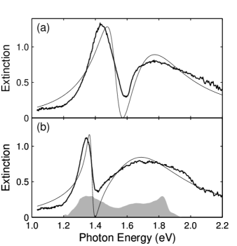
Figure 6: Extinction of the selected samples (a) A and (b) B. The thick curves show the extinction measured with a white-light source, referenced to the substrate without gold structures. The thin lines are absorption spectra derived from the model of coupled Lorentz oscillators, Eq. (13), obtained by a nonlinear least-squares fit to the corresponding experimental data. The gray area in (b) depicts the electric field spectrum (square root of the measured intensity spectrum) of the laser pulses used for the nonlinear-optical experiments.

To connect to theory, the measured extinction spectra (negative logarithm of the intensity transmittance, referenced to the substrate without gold structures) for TM polarization and for normal incidence are compared with Eq. (13) derived in Sec. III (see Fig. 6). In these experiments we use a white-light source focused with a numerical aperture (NA) of about 0.025. Using a yet smaller NA tends to make the extinction dip even more pronounced. A careful discussion of this aspect can be found in Ref. ChristPRB04, . We find a good qualitative agreement of our simple theoretical model and the experiments. From a least-squares fit of the theory to the experiment (see Fig. 6) we obtain all relevant parameters, leaving only the nonlinear coefficients $\eta_{k}$ as free parameters for the nonlinear-optical experiments to come. The experimental parameters of sample A (B) are: $a=550\,\rm nm$, $w=185\pm 5\,\rm nm$ ($a=625\,\rm nm$, $w=195\pm 5\,\rm nm$). The fit parameters of sample A (B) are: $\hbar\Omega_{\rm pl}=1.67\,\rm eV$, $\hbar\Omega_{\rm wg}=1.56\,\rm eV$, $\hbar\Omega_{\rm c}=0.66\,\rm eV$, $\tau=1.06\,\rm fs$, and $q_{\rm wg}/q_{\rm pl}=+0.085$ ($\hbar\Omega_{\rm pl}=1.65\,\rm eV$, $\hbar\Omega_{\rm wg}=1.39\,\rm eV$, $\hbar\Omega_{\rm c}=0.54\,\rm eV$, $\tau=0.97\,\rm fs$, and $q_{\rm wg}/q_{\rm pl}=+0.049$), where $\tau=1/(2\gamma)$. The additional fit parameter $\alpha_{\rm pl}$, together with the coefficients $\eta_{k}$, determines the absolute strength of the THG signals. Sample A is resonant, i.e., $\hbar|\Omega_{\rm pl}-\Omega_{\rm wg}|=0.11\,{\rm eV}<0.27\,{\rm eV}=\hbar\Omega_{\rm c}^{2}/\widehat{\Omega}$, while sample B is nonresonant, i.e., $\hbar|\Omega_{\rm pl}-\Omega_{\rm wg}|=0.26\,{\rm eV}>0.19\,{\rm eV}=\hbar\Omega_{\rm c}^{2}/\widehat{\Omega}$ (see discussion in previous section).

V.2 Nonlinear-optical experiments

In our THG experiments, we use 5 fs laser pulses derived from a laser system closely similar to the one described in Ref. MorgnerOL99, ($81\,\rm MHz$ repetition frequency). The pulses are sent into a Michelson interferometer, which is actively stabilized by means of the “Pancharatnam screw.”WehnerOL97 The linearly polarized pulses emerging from the interferometer are focused onto the samples (normal incidence and TM polarization) by a spherical mirror with a focal length of $f=100\,\rm mm$. To estimate the intensities in the spot and to determine the effective NA, we have measured the spot size and the Rayleigh length by a knife-edge method in the horizontal (vertical) direction. The determined spot radius of $12.5\,(12.3)\,\rm\mu m$ is significantly smaller than the size of the nanowire arrays and leads to a pulse intensity around $I=3.9\times 10^{10}\,\rm W/cm^{2}$ and a laser fluence of $200\,\rm\mu J/cm^{2}$ used in the experiments described below (for an average power of 80 mW in front of the sample). We will argue later that this fluence is still within the third-order perturbational limit. The corresponding Rayleigh lengths of $490\,(560)\,\mu$m lead to an effective NA of 0.025 (0.022).

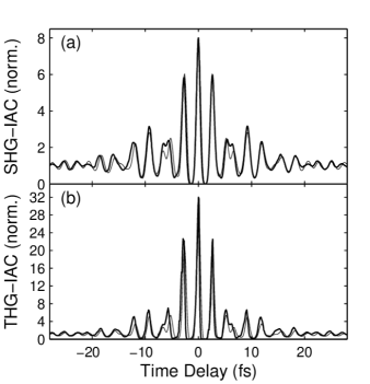
Figure 7: Characterization of the $5\,\rm fs$ laser pulses. (a) Second-order interferometric autocorrelation (SHG-IAC) measured directly (thick line) and calculated (thin line) from the measured pulse spectrum under the assumption of a flat spectral phase. (b) Third-order interferometric autocorrelation (THG-IAC) measured directly (thick line) and calculated (thin line) in analogy to (a).

In Fig. 7 we depict the characterization of the laser pulses. The thick curve in (a) shows the usual second-order autocorrelation obtained from a very thin $\beta$-barium-borate SHG crystal. The thin line is the autocorrelation as calculated from the measured laser spectrum [see gray area in Fig. 6(b)] under the assumption of a spectrally flat phase. The good agreement indicates that the residual chirp on the 5 fs pulses is of minor importance. The thick curve in Fig. 7(b) shows the third-order autocorrelation function measured via THG from the surface of a thick sapphire plate. The thin curve in (b) is the corresponding calculated response under the same assumptions as in (a). Again, the agreement is very good. Notably, the envelope of the THG signal has decayed by a factor of 4 for time delays of just two cycles of light. These curves in (b) can be considered as the apparatus function and have to be compared with the measurements to be discussed in what follows. The achieved ratio of 32:1 between the THG signal at zero time delay and large time delays, respectively, indicates good alignment of the interferometer.

In the THG experiments, the emission from the samples in the forward direction is collected by another spherical mirror (focal length $f=100\,\rm mm$), spectrally prefiltered by means of four fused-silica Brewster-angle prisms to suppress the overwhelming fundamental laser light and spectrally resolved using a 0.5-m-focal-length grating spectrometer (with a grating blazed at 250 nm wavelength) connected to a uv-sensitive, back-illuminated, liquid-nitrogen-cooled charge-coupled-device camera.

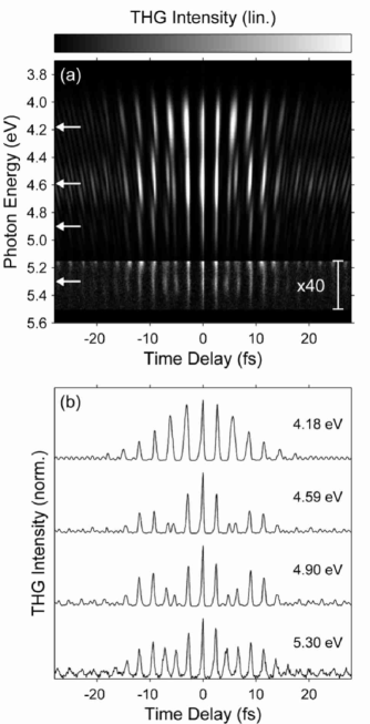
Figure 8: (a) Measured THG intensity from sample A. The THG intensity is shown on a saturated gray scale, versus spectrometer photon energy and interferometric time delay. Near time delay $T=0$, the THG spectrum exhibits four peaks (the weak high-energy peak is amplified by a factor of 40 to become visible). The four peaks exhibit a different temporal behavior. Corresponding cuts at the spectral peak positions indicated by the white arrows in (a) are shown in (b). For better comparison, the curves are normalized to the same maximum and are vertically displaced. The appearance and absence of beating is discussed in the text. Compare with the corresponding theory (Fig. 3).

Figure 8 shows a typical data set of sample A, containing 600 individual spectra obtained in a total of about 8 min acquisition time. Here, the THG signal is plotted on a linear gray scale as a function of spectrometer photon energy and time delay. The exact same representation has already been employed in the theory Sec. (see Figs. 3 and 4). Indeed, the linear-optical parameters of Figs. 3 and 4 correspond to those of sample A [compare linear spectra in Fig. 6(a)]. Obviously, the measured nonlinear-optical spectra are much closer to those in Fig. 3 than to any of Fig. 4. In particular, four peaks occur in the spectra at zero time delay. Also, the dependencies of the different spectral cuts versus time delay in Fig. 8(b) closely resemble those in Fig. 3(b). Again, the envelopes of the first and fourth cuts show hardly any beating, whereas the envelopes of the second and third cuts reveal a pronounced beating behavior [note that the very weak fourth peak in Fig. 8(a) spectrally overlaps with the wing of the third peak, resulting in a small residual beating]. This comparison allows us to conclude that the nonlinear model where only $\eta_{0}$ is nonzero is the appropriate one. This means that the nonlinearity predominantly originates from the particle plasmon – which is not a priori clear. This finding is consistent with the experimental finding that the nonlinear signal decreases by a factor of 19 (and the multi-peak features disappear) when going from the TM polarization used so far to the TE polarization. It is also consistent with the fact that the THG signals drop by a factor of about 20 when going from the gold nanowire arrays to areas of the glass substrate where only the dielectric layers are present.

It is important for our interpretation that the experiments are performed in the third-order perturbation regime – which is also assumed in the theoretical analysis. Higher-order contributions would obviously modify the ratio of 32:1 between the THG signal at zero time delay and that at large time delays. In the experiments, the ratio of 32:1 is reached within experimental uncertainty: From analyzing the upper (lower) envelope of spectrally integrated data like those shown in Fig. 8 but for time delays up to $\pm 60\,\rm fs$, we derive a ratio of 24:1 (35:1). The actual ratio – which refers to a comparison between zero and infinite time delay – must lie between these two ratios.

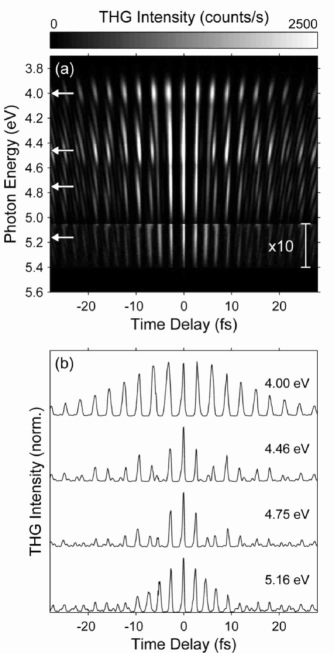
Figure 9: (a) Measured optical THG intensity from sample B. Near $T=0$, the THG spectrum clearly exhibits four peaks (the high-energy peak is amplified by a factor of 10). Normalized cuts at the spectral peak positions indicated by the white arrows in (a) are shown in (b). Note the much slower, smooth decay of the envelope of the cut at $4.00\,\rm eV$ as compared to the cut at $5.16\,\rm eV$, and the beating, which only occurs in the other two curves.

In Fig. 9, we show the data set for the “nonresonant” sample B. As for sample A, four spectral peaks are visible in the THG spectra. In contrast, however, the peaks in Fig. 9(a) have rather different spectral widths, as expected from the fact that the two effective extinction peaks [see Fig. 6(b)] exhibit rather different spectral widths and our discussion of Sec. IV. The different spectral widths in Fig. 9(a) correspond to strongly different decay times of the envelopes in Fig. 9(b). Again, only the envelopes of the first and fourth cuts show a smooth decay, whereas the envelopes of the second and third cuts exhibit a pronounced beating.

VI Conclusions

We have investigated the linear- and nonlinear-optical lineshapes of metal nanoparticles and metallic photonic crystal slabs.

For particle ensembles, we have shown analytically and numerically that the comparison of time-resolved femtosecond second- or third-harmonic-generation experiments and extinction measurements does not allow one to distinguish between homogeneous and inhomogeneous contributions to the linewidth. Optical-rectification or four-wave-mixing experiments would provide such information.

For metallic photonic crystal slabs, we have demonstrated that the model of two coupled Lorentz oscillators describes very well the key experimental features of linear optics. In particular, Fano-like lineshapes appear in the absorption spectra. With regard to nonlinear optics, we have shown that – within the regime of “moderate coupling” – the nonlinear-optical third-harmonic-generation spectra provide information on the underlying source of the optical nonlinearity. Furthermore, the calculated nonlinear spectra reveal a beating in the spectral mixing products of the two peaks from linear optics, but not in the third harmonics of the latter peaks.

Our corresponding experiments on third-harmonic generation of metallic photonic crystal slabs go beyond previous work regarding improved temporal resolution and the fact that we spectrally resolve the interferometric third-harmonic signal. The spectra reveal a distinct behavior of the various spectral components versus time delay. Some spectral components exhibit a beating, others do not. Furthermore, the decay times of the envelopes strongly depend on the spectral component. The measured spectra agree qualitatively very well with the predictions of the simple theoretical model. The comparison allows us to identify the particle plasmon oscillation as the main source of nonlinearity.

- (1) U. Kreibig and M. Vollmer, Optical Properties of Metal Clusters (Springer-Verlag, Berlin, 1995).
- (2) M. Nevière, in Electromagnetic Theory of Gratings, edited by R. Petit (Springer-Verlag, Berlin, 1980), Chap. 5, pp. .
- (3) S. Linden, J. Kuhl, and H. Giessen, Phys. Rev. Lett. 86, 4688 (2001).
- (4) A. Christ, S. G. Tikhodeev, N. A. Gippius, J. Kuhl, and H. Giessen, Phys. Rev. Lett. 91, 183901 (2003).
- (5) T. Zentgraf, A. Christ, J. Kuhl, and H. Giessen, Phys. Rev. Lett. 93, 243901 (2004).
- (6) B. Lamprecht, J. R. Krenn, A. Leitner, and F. R. Aussenegg, Appl. Phys. B: Lasers Opt. 69, 223 (1999).
- (7) B. Lamprecht, G. Schider, R. T. Lechner, H. Ditlbacher, J. R. Krenn, A. Leitner, and F. R. Aussenegg, Phys. Rev. Lett. 84, 4721 (2000).
- (8) B. Lamprecht, J. R. Krenn, A. Leitner, and F. R. Aussenegg, Phys. Rev. Lett. 83, 4421 (1999).
- (9) G. Schider, J. R. Krenn, A. Hohenau, H. Ditlbacher, A. Leitner, F. R. Aussenegg, W. L. Schaich, I. Puscasu, B. Monacelli, and G. Boreman, Phys. Rev. B 68, 155427 (2003).
- (10) T. Vartanyan, M. Simon, and F. Träger, Appl. Phys. B: Lasers Opt. 68, 425 (1999).
- (11) F. Stietz, J. Bosbach, T. Wenzel, T. Vartanyan, A. Goldmann, and F. Träger, Phys. Rev. Lett. 84, 5644 (2000).
- (12) M. J. Weida, S. Ogawa, H. Nagano, and H. Petek, J. Opt. Soc. Am. B 17, 1443 (2000).
- (13) C. Sönnichsen, T. Franzl, T. Wilk, G. von Plessen, J. Feldmann, O. Wilson, and P. Mulvaney, Phys. Rev. Lett. 88, 077402 (2002).
- (14) H. G. Craighead and G. A. Niklasson, Appl. Phys. Lett. 44, 1134 (1984).
- (15) M. Volmer and A. Weber, Z. Phys. Chem. (Leipzig) 119, 277 (1926).
- (16) B. Lamprecht, A. Leitner, and F. R. Aussenegg, Appl. Phys. B: Lasers Opt. 64, 269 (1997).
- (17) The same problem associated with Eq. (4) can arise for a conventional interferometric autocorrelation of laser pulses (Ref. DielsBook ), where one has . There, however, the IAC remains unaffected, provided that the negative-frequency part of the laser spectrum has negligible overlap with the positive-frequency part.
- (18) Jean–Claude Diels and Wolfgang Rudolph, Ultrashort Laser Pulse Phenomena (Academic Press, London, 1996), Chap. 8.
- (19) M. Wegener, D. S. Chemla, S. Schmitt -Rink, and W. Schäfer, Phys. Rev. A 42, 5675 (1990).
- (20) A. Sharon, D. Rosenblatt, and A. A. Friesem, J. Opt. Soc. Am. A 14, 2985 (1997).
- (21) U. Fano, Phys. Rev. 124, 1866 (1961).
- (22) H. Giessen, S. Linden, A. Christ, J. Kuhl, D. Nau, T. Meier, P. Thomas, and S. W. Koch, in International Quantum Electronics Conference (IQEC), IFC5, San Francisco, 2004.
- (23) Fitting the square root of the measured laser spectrum (spectral intensity) with a sum of three Gaussians, we model the electric field spectrum with , where , , , , , , , and (compare with gray area in Fig. 6). In the time domain, this corresponds to .
- (24) A. Christ, T. Zentgraf, J. Kuhl, S. G. Tikhodeev, N. A. Gippius, and H. Giessen, Phys. Rev. B 70, 125113 (2004).
- (25) U. Morgner, F. X. Kärtner, S. H. Cho, Y. Chen, H. A. Haus, J. G. Fujimoto, E. P. Ippen, V. Scheuer, G. Angelow, and T. Tschudi, Opt. Lett. 24, 411 (1999).
- (26) M. U. Wehner, M. H. Ulm, and M. Wegener, Opt. Lett. 22, 1455 (1997).