Hydrodynamic induced deformation and orientation of a microscopic elastic filament

Abstract

We describe simulations of a microscopic elastic filament immersed in a fluid and subject to a uniform external force. Our method accounts for the hydrodynamic coupling between the flow generated by the filament and the friction force it experiences. While models that neglect this coupling predict a drift in a straight configuration, our findings are very different. Notably, a force with a component perpendicular to the filament axis induces bending and perpendicular alignment. Moreover, with increasing force we observe four shape regimes, ranging from slight distortion to a state of tumbling motion that lacks a steady state. We also identify the appearance of marginally stable structures. Both the instability of these shapes and the observed alignment can be explained by the combined action of induced bending and non-local hydrodynamic interactions. Most of these effects should be experimentally relevant for stiff micro-filaments, such as microtubules.

Semi-flexible polymers and filaments are important components of biological systems. All cytoskeletal filaments, used by cells for transport, morphology and force generation, fall into this category How01 . So do their assemblies, cilia and flagella, used to generate propulsion Grey1955 ; Lowe2003 . Recent developments in experimental techniques allow the controlled synthesis, manipulation and direct visualization of both real Goldstein ; chu ; Stracke2002 and model filaments Gast2004 of this type. Consequently, there is renewed interest in the theory and simulation of both their static and dynamic properties, the structure and dynamics of DNA in flows chu for example. If one is interested in dynamics, as we are here, one must consider that these filaments are normally suspended in a fluid. On the micron scale, inertia is generally negligible; any motion takes place in an environment effectively a billion times stickier than we experience in our daily lives Purcell . The dynamic response is determined by both elastic and fluid forces. Analytically, this is a non-trivial nonlinear problem. Nonetheless, at the linearized level the case of an elastic filament waved at one end has been solved Goldstein , and the predictions compared successfully with micro-manipulation experiments on an actin filament. The fluid was accounted for by introducing friction coefficients for parallel and perpendicular filament motion, independent of both the location along the filament and its configuration. Such an approximation is termed resistive force theory Grey1955 and is satisfactory for several problems. Given experimentally observed flagella waveforms it gives good predictions for the swimming speed of spermatozoa Lowe2003 . It also predicts the buckling instability Shelley2001 observed in sheared suspensions of filaments.

However, resistive force theory is an approximation. In reality, a moving filament sets up spatially varying flow fields in the fluid that couple back to the motion of the filament itself. To see why this coupling need not be trivial, suppose we approximate a filament of length $L$ as a set of $n$ beads separated by a fixed distance $b=L/(n-1)$, in the spirit of the “shish kebab” model Doi of a cylinder. A bead moving with velocity ${\bf v}$ experiences a hydrodynamic frictional force ${\bf F}_{\rm H}=-\gamma_{0}({\bf v}-{\bf v}_{\rm H})$, where $\gamma_{0}$ is a bead friction coefficient and ${\bf v}_{\rm H}$ is the velocity of the fluid at the location of the bead. Writing ${\bf v}_{\rm H}$ in terms of the flow fields of the other beads gives the hydrodynamic force on bead $i$

$${\bf F}_{i{\rm H}}=-\gamma_{0}{\bf v}_{i}+\frac{\gamma_{0}}{8\pi\eta}\sum_{j\neq i}\left[\frac{{\bf F}_{j}}{r_{ij}}+{\bf F}_{j}\cdot\frac{{\bf r}_{ij}{\bf r}_{ij}}{{r_{ij}}^{3}}\right]\,$$ (1)

where ${\bf r}_{ij}$ is the vector connecting beads $i$ and $j$, ${\bf F}_{j}$ the non-hydrodynamic force acting on bead $j$ and $\eta$ the viscosity of the fluid oseen . Consider now a filament subject to a uniform external force density $\tilde{F}^{\rm x}$ directed perpendicular to the axis of the rod (all forces and velocities are in the plane defined by the rod and the external force). If $b<<L$ equation (1) gives

$$F_{{\rm H}}(s)=-\gamma_{0}\left[v(s)-\frac{\tilde{F}^{\rm x}}{8\pi\eta}\ln{\frac{s(L-s)}{b^{2}}}\right]$$ (2)

where $s\in[0,L]$ is the distance along the filament. The second term in the bracket is due to the non-local flow created by the rest of the beads. For a rigid body, the velocity is a constant, while the hydrodynamic friction force is greater towards the ends of the rod than in the middle. Thus, one expects a flexible filament to bend. In this letter, we examine this problem numerically and show that this spatially varying interaction between the filament and the fluid substantially enriches the dynamic behavior of the system. Notably, the simulations predict hydrodynamic induced distortion and orientation that should be observable experimentally.

We describe results from a simple numerical model that takes into account the interaction of the filament with its surrounding fluid more realistically than the resistive force approximation. The position-dependent frictional forces are calculated explicitly from the flow fields generated by the filament and will generally be configuration dependent and non-uniform. The semiflexible filament is treated as a curve, with its instantaneous configuration specified by a position vector ${\bf r}(s)$. The length is fixed and the elastic energy characterized by a Hamiltonian $H=\kappa\int_{0}^{L}C(s)^{2}ds/2$ Christopher , where $C(s)=|\partial^{2}{\bf r}/\partial s^{2}|$ is the local curvature and $\kappa$ the stiffness. Numerically, the filament is modeled as a set of rigidly connected beads. The force acting on a bead is the sum of the external, tension, bending and hydrodynamic force. We calculate the latter from eq. (1), with ${\bf F}_{j}$ being the sum of all non-hydrodynamic forces acting on bead $j$. We can use eq. (2) to calculate the friction coefficients of a rigid filament modeled to this degree of approximation, yielding the friction coefficient $\gamma^{\perp}$ for motion perpendicular to the rod $\gamma^{\perp}={4\pi\eta L}/{\ln{\left(L/b\right)}}$, in the limit $b<<L$ gammaperp . If the bead spacing is interpreted as the cylinder radius this result is the same as the exact slender body hydrodynamic theory for a cylinder limitation . An advantage of our approach is that, despite its simplicity, with increasing number of beads it approaches the correct result for a slender body, including the non-local nature of the hydrodynamic forces. It is accurate for very slender filaments and most of the biofilaments we are interested in satisfy this condition. Although a mathematically more sophisticated approach to treat the slender limit exists shelley2 , it does not account for the fact that the hydrodynamic force for a filament under a uniform field need not be uniform. As the force on a particle due its hydrodynamic interaction with its neighbors depends only on the external force and the instantaneous configuration of the filament, the simple implicit method described in ref. Lowe2003 suffices to integrate the equations of motion. These are solved subject to the condition that filament inertial effects are irrelevant (the motion is overdamped, consistent with neglecting the fluid inertia).

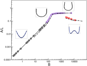
Figure 1: Bending amplitude $A$, as a function of the the dimensionless force $B$, for a filament with $L/b=30$ (solid line) and $L/b=100$ (dashed line). The insets are the corresponding shapes (the external force acts in the downward direction).

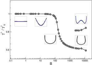
Figure 2: The perpendicular friction coefficient, $\gamma^{\perp}$, relative to its value in the stiff limit $\gamma^{\perp}_{0}$, as a function of the dimensionless force $B$.

We first consider the motion of a filament under the action of a uniform field $\tilde{F}^{\rm x}$, acting perpendicular to the axis of an initially straight filament. The filament’s shape evolves in time until a steady state is reached, where it drifts at a constant velocity with a fixed shape. That is, the bending, external and tension forces are balanced by the configuration dependent fluid force at every point along the filament. This steady state is a function of a dimensionless force $B=L^{3}\tilde{F}^{\rm x}/\kappa$. When $B<<1$, we expect the filament to behave as a rigid rod. With increasing $B$, significant bending will be required to balance any non-uniformity in the hydrodynamic force. Typical shapes we observe for the steady state over a range of values of $B$ are shown inset in Fig. 1. In the steady state the filament is bent, indicating that the higher frictional force towards the end of the filament has to be balanced by a bending force. In the figure we plot a characteristic transverse distortion, $A$, defined as the distance between the uppermost and lowermost point of the filament along the direction of the applied force. We can identify four distinct regimes. For forces corresponding to small values of $B$ $(B<50)$, the degree of distortion is small and increasing in proportion to $B$. This is the linear regime, where the bending can be understood as one of the lowest elastic modes Goldstein ; check excited in response to the applied force (coming both from the external field and hydrodynamic interactions). For $B>100$ the coupling between hydrodynamic and elastic forces is clearly non-linear, as evidenced by the rounded “U” shape of the filament in this regime. The bending amplitude saturates and, with increasing $B$, the filament “U” shape becomes increasingly rounded. In this regime we also see that the friction coefficient starts to markedly decrease, as shown in Fig. 2. This is because the progressive alignment of the filament with the applied force leads to an increasing fraction of parallel motion (see Fig. 1), characterized by a lower friction. The perpendicular friction coefficient is always greater than the parallel friction coefficient (not shown) but, for large $B$, appears to approach it parallel . Thus, in this limit the filament approaches hydrodynamically isotropic behavior. For even higher values of $B$, $(B>2000$), we see yet different behavior. The filament initially adopts a new “W” shape, that, incidentally, has a more uniform hydrodynamic force density (and hence is closer to resistive force theory) and a lower distortion (shown by the lower data points in the figure) than its final state. The W configuration is marginally stable; for any initial perturbation, after a transient time the W configuration rotates with the same handedness as the original perturbation and finally adopts a highly distorted but stable “horse shoe” shape (the upper data points shown in Fig. 1). At still higher $B$ ($>4000$), we observe a regime (not shown) where following the formation of the “W” the filament again rotates but never adopts a new stable state. Rather, it exhibits a periodic zig-zagging motion indicating that above some critical value of $B$ there is no dynamically stable steady state that the filament can reach movies .

Now we consider a filament that is initially straight but with its axis tilted with respect to the force. If the hydrodynamic friction along the rod is uniform, the filament will remain straight and maintain the same orientation. It will move at the constant velocity for which the friction and external forces balance each other dhont . Because the parallel and perpendicular friction coefficient differ, this will generally be at an angle to the external force. A truly rigid rod, even with non-local hydrodynamic interactions, must also move at constant speed maintaining its initial orientation, as is the case for any rigid object. However, as shown in Fig. 3, we find that if the initial configuration is rotated anti-clockwise with respect to the external force, as the rod translates it rotates clockwise until its ends are again aligned perpendicular to the force. During the rotation the filament exhibits a transient drift motion in a direction inclined to the force but in the steady state, unlike a rigid rod, the drift is along the applied force direction. We recover identically the case discussed above.

The orientation angle as a function of time - after a time during which bending is established - decays exponentially thesis . The characteristic time for this decay, $\tau_{\rm H}$, relative to the time a rigid rod takes to translate its length ($\tau_{\rm T}=\gamma^{\perp}/\tilde{F}^{\rm x}$) is plotted as a function of $B$ in Fig. 3.

This effect is related to the flexibility, because a truly rigid rod cannot display this behavior. Why should a flexible filament behave so differently? As long as the rod is not aligned parallel to the applied force, there is a component of the force perpendicular to the filament inducing bending. Taking the situation illustrated in Fig. 3, the bending will slightly align the tangent to the filament at the right hand end parallel to the applied force and the tangent at the left hand end perpendicular. The local friction coefficient is higher perpendicular to the filament than parallel. So, even if the two ends move with the same velocity, the drag force on the right hand end will be slightly lower that that on the left. Thus, a torque tends to rotate the filament clockwise, as we observe (see Fig. 3). A simple semi-quantitative analysis indicates that in the linear regime, where the degree of bending is proportional to $B$, the torque generated is proportional to $B$. One therefore expects that the time it takes the filament to reorient scales as $1/B$, as shown in Fig. 3. Note that this simple argument only invokes the non-local hydrodynamics to generate the bending that breaks the symmetry between the two ends. Arguing along the same lines, resistive force level hydrodynamics predicts rotation of a bent filament. It fails because it does not include the mechanism that generates the bending.

This analysis has some interesting consequences. It appears that any degree of elasticity will induce the rotation of the filament. Hence, the completely rigid limit is singular, in the sense that the absence of orientation is because the reorientation time becomes indefinitely long as the rigidity increases. It also implies that the motion of a flexible filament aligned parallel to the force will be unstable. A small perturbation of the angle from the parallel, with a certain handedness, generates a torque with the same handedness. The perturbation will be amplified and the filament will rotate until the dynamically stable perpendicularly aligned “U” state is reached. This reasoning also explains why the “W” shape is marginally stable. By symmetry, the two outer “U” sections cannot contribute any net torque. However, the central convex section will display an instability with respect to any perturbation from the perpendicular, consistent with our observation that the “W” configuration eventually rotates to form a horse shoe.

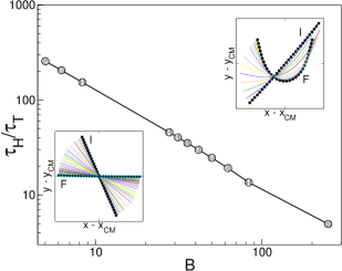
Figure 3: Log-log plot of the characteristic hydrodynamic re-orientation time relative to the translational time, $\tau_{\rm H}$, as a function of the dimensionless force $B$. Inset are the corresponding motions for two characteristic values of B, viewed in the center of mass frame of reference, the initial and final states being $I$ and $F$ respectively (the external force acts in the downward direction).

Could this behavior be relevant in practice? Appreciable bending requires $B>>1$ while hydrodynamic induced rotation should occur for any value of $B$ (although for small $B$ the reorientation time will be long). In the case of biofilaments, a gravitational field only gives low values of $B$. Microtubules have a stiffness of $\kappa\sim 50pN\mu m^{2}$ Jans_Dog04 , so for a typical length ($10\mu m$) we estimate that $B<10^{-3}$. Accelerations three orders of magnitude greater than gravity are needed to reach even $B\sim 1$ (which can be achieved in a centrifuge). However, bio-filaments are commonly charged, and hence will react to applied electric fields. If we concentrate on microtubules, they are negatively charged with an effective charge density $\tilde{q}$ of approximately $200e/\mu m$ Stracke2002 , where $e$ is the elementary charge. The strongest electric fields for which microtubules are stable, reported in ref Stracke2002 , are of order $10^{4}V/m$, corresponding to a force density of $0.3pN/\mu m$. For a microtubule of length $L\sim 5\mu m$ (as used in the experiments reported in Stracke2002 ) one then finds $B\sim 1$. However, since $B\propto L^{3}$ for longer microtubules of $L\sim 30\mu m$, we have $B\sim 200$. It is therefore possible to apply forces that should induce observable bending. A further condition to observe the orientational behavior we describe is that the hydrodynamic orientational time $\tau_{\rm H}$ is shorter than any other relaxation time in the problem. For example, we have thus far ignored rotational diffusion. It will tend to randomize the orientation on a characteristic time scale $\tau_{D}\sim\gamma^{\perp}L^{2}/kT$. From Fig. 3 we see that $\tau_{\rm H}\sim\gamma^{\perp}/(\tilde{F}^{\rm x}B)$, so $\tau_{\rm H}/\tau_{D}\sim L/(B^{2}\lambda$), where $\lambda(=\kappa/kT)$ is the persistence length. One can therefore neglect diffusion if $L/(B^{2}\lambda)<<1$. For a stiff filament, $L/\lambda<<1$ (for a $10\mu m$ microtubule this ratio is $10^{-2}$), so this condition is automatically satisfied if $B\geq 1$. In addition, microtubules have an electric dipole. This will lead to a torque tending to align them parallel to the electric field while they translate and bend. The ratio of the dipole re-orientation time $\tau_{\rm d}$ to the translational time is $\tau_{\rm d}/\tau_{\rm T}=\tilde{q}L^{2}/d$, where $d$ is the electric dipole. Experimental results indicate that $d\sim eL$  Stracke2002 . Hence the ratio is $\tau_{\rm d}/\tau_{\rm T}\sim 200L/\lambda_{\rm d}$ with the length $\lambda_{\rm d}=1\mu m$. So for a microtubule with $L>1\mu m$ the dipolar re-orientation should be negligible compared to hydrodynamic orientation.

An analysis along these lines suggests that for actin and DNA it is possible to achieve $B>>1$. However, the condition that the hydrodynamic orientation time is shorter than all other time-scales is not easily satisfied. There will be a competition between the effects we describe here, acting to distort and align the filament, and thermal effects, acting to randomize the orientation and maintain the equilibrium structure. Finally, the situation with carbon nanotubes is more flexible, given the greater control of physical properties of these objects nanotubes . It may be possible to reach the $B>>1$ regime where the instability sets in.

In this letter we have shown how the non-local nature of the hydrodynamic interactions affects the dynamics of inextensible elastic filaments subject to a uniform external field. The method captures all the relevant configurational couplings. Although the hydrodynamic treatment is only exact for an infinitely slender rod, it is computationally simple compared to other techniques shelley2 ; sd . The non-uniform, configuration-dependent friction the fluid exerts on the filament induces distortion and a corresponding increase in mobility. In the dynamic steady state, the degree of bending depends on the stiffness of the filament, a fact that could be used experimentally to determine $\kappa$. There is a crossover from the linear regime to a plateau value for the degree of distortion, reminiscent of other pattern-forming systems. Our numerical results suggest that at still higher degrees of forcing there exist long-lived marginally stable states and that eventually the filament behaves in an unsteady but hydrodynamically isotropic manner. The fact that fluid friction induces bending means that a flexible rod aligns perpendicular to an applied force. This is not expected if one neglects either the flexibility of the filament or the non-local hydrodynamics. It does, however, offer a novel route by which one may manipulate the orientations of filaments experimentally.

- (1) J. Howard, “Mechanics of Motor Proteins and the Cytoskeleton”. Sinauer Press MA (USA) (2001).
- (2) J. Grey and G. Hancock, J. Exp. Biol. 32, 802 (1955).
- (3) C.P. Lowe, Phil. Trans. R. Soc. Lond. B358 , 1543 (2003).
- (4) C.H. Wiggins, D. Riveline, A. Ott and R.E. Goldstein, Biophys. J. 74, 1043 (1998).
- (5) C.M. Schroeder, H.P. Babcock, E.S.G. Shaqfeh and S. Chu, Science 301, 1515 (2003).
- (6) R. Stracke, K.J. Böhm, L. Wollweber, J.A. Tuszynski and E. Unger, Biophys. Res. Commun. 293, 602 (2002).
- (7) C. Goubault, P. Joy, J. Baudry, E. Bertrand, M. Fermigier and J. Bibette, Phys. Rev. Lett. 91 (2003) 260802; S.L. Biswal and A.P. Gast, Phys. Rev. E69, 041406 (2004).
- (8) M.E. Purcell, Am.J.Phys. 45, 3-11 (1977).)
- (9) L. E. Becker and M. J. Shelley, Phys. Rev. Lett. 87, 198301 (2001)
- (10) M. Doi and S.E. Edwards, “The dynamics of polymer solutions”, Cambridge University Press (1986).
- (11) By using the Oseen tensor we disregard the beads’ size and consider them hydrodynamically as points of force.
- (12) M. Cosentino Lagomarsino, F. Capuani and C.P. Lowe, J. Theor. Biol. 224, 215 (2003).
- (13) The friction coefficient is defined as the ratio of the total external force acting on a straight filament to an imposed uniform drift velocity. Using the same definition, the parallel friction coefficient is , again consistent with slender body theory.
- (14) Our model cannot represent cylindrical filaments with a given aspect ratio using a variable number of beads. This requires an explicit filament/fluid interface which is computationally much more demanding.
- (15) A.-K. Tornberg and M.J. Shelley, J. Comput. Phys. 196, 8 (2004).
- (16) We verified that for small amplitudes the elastic modes can be projected onto the known elastic eigenmodes of the filament.
- (17) The parallel friction coefficient is computed from a straight configuration parallel to the field, before any instability occurs.
- (18) Animations of the simulations can be viewed at http://www.science.uva.nl/macromol/filament.php
- (19) J.K.G. Dhont, An Introduction to Dynamics of Colloids (Studies in Interface Science) (Elsevier, 1996)
- (20) M. Cosentino Lagomarsino, Ph.D. Thesis, Amsterdam (2004).
- (21) M.E. Janson and M. Dogterom, Biophys J. 87 2723 (2004).
- (22) S. Lin-Gibson, J.A. Pathak, E.A. Grulke, H. Wang and E.K. Hobbie, Phys. Rev. Lett. 92, 048302 (2004).
- (23) R. Kutteh, J. Chem. Phys. 119, 9280 (2003).