The field theory of symmetrical layered electrolytic systems and the thermal Casimir effect

Abstract

We present a general extension of a field-theoretic approach developed in earlier papers to the calculation of the free energy of symmetrically layered electrolytic systems which is based on the Sine-Gordon field theory for the Coulomb gas. The method is to construct the partition function in terms of the Feynman evolution kernel in the Euclidean time variable associated with the coordinate normal to the surfaces defining the layered structure. The theory is applicable to cylindrical systems and its development is motivated by the possibility that a static van der Waals or thermal Casimir force could provide an attractive force stabilising a dielectric tube formed from a lipid bilayer, an example of which are t-tubules occurring in certain muscle cells. In this context, we apply the theory to the calculation of the thermal Casimir effect for a dielectric tube of radius $R$ and thickness $\delta$ formed from such a membrane in water. In a grand canonical approach we find that the leading contribution to the Casimir energy behaves like $-k_{B}TL\kappa_{C}/R$ which gives rise to an attractive force which tends to contract the tube radius. We find that $\kappa_{C}\sim 0.3$ for the case of typical lipid membrane t-tubules. We conclude that except in the case of a very soft membrane this force is insufficient to stabilise such tubes against the bending stress which tend to increase the radius. We briefly discuss the role of lipid membrane reservoir implicit in the approach and whether its nature in biological systems may possibly lead to a stabilising mechanism for such lipid tubes.

1 Introduction

In an recent short communication we reported on a calculation which investigated the the possibility that a static van der Waals or thermal Casimir force could provide an attractive force across a tube formed from a lipid bilayer, so leading to its stabilisation. In this paper we give the details of the general theory of symmetrically layered electrolytic systems which underlies that calculation, and explain the details of the calculation applying the theory to cylindrical geometry and to a model for the lipid bilayer tube. Whilst the motivation for developing the theory presented below is the analysis of the the Casimir force in the context of a dielectric tube immersed in water, the theory is applicable to any sufficiently symmetrical system consisting of layer containing electrolyte. The Coulomb properties of such systems are described by a Sine-Gordon field theory and a full analysis in the case of flat layers has been done with the approach which is generalised in this paper. In particular, it allows for the perturbation series for the thermal Casimir force to be developed in terms of the dimensionless coupling $g=l_{B}/l_{D}$ where $l_{B}$ and $l_{D}$ are the Bjerrum and Debye lengths, respectively.

The behaviour of systems composed of layer of varying dielectric constants was first studied by Lifshitz and coworkers [1] and has been subsequently revisited by a number of authors [2, 3, 4]. The formalism developed is an elegant way of taking into account van der Waals forces in a continuum theory. Two types of van der Waals forces are accounted for in theses theories, firstly zero frequency van der Waals forces whose nature is purely classical and secondly the frequency dependent ones due to temporal dipole fluctuations. In terms of thermal field theory the former correspond to the zero frequency Matsubara frequency and the latter to the non zero frequencies. In order to calculate these latter terms we require information about the frequency dependence of the dielectric constants, where as the former only requires the static dielectric permittivity. The quantum Casimir effect corresponding to the modification of the ground state energy of the electromagnetic field has been intensively studied in the case of idealised boundary conditions in a variety of geometries including spheres and cylinders [5]. The thermal Casimir effect investigated here has a similar mathematical structure though the corresponding effective spatial dimension is one less in the calculations. The temperature dependence of the full Casimir in a simplified model of a solid dielectric cylinder (and sphere) has been recently examined using a heat kernel coefficient expansion [6]. In our analysis of the diffuse limits we make use of summation theorems for Bessel functions which were introduced for the study of the Casimir energy for cylinders with light-velocity conserving boundary conditions [7]. In this paper we will calculate only the zero frequency contribution, also known as the thermal Casimir effect. The thermal Casimir effect may also be calculated in the presence of electrolyte and the technique we develop here for electrolytic systems within the Debye Hückel approximation is valid in the domain of weak electrolyte concentrations. There is an extensive literature on the thermal Casimir effect for systems of layered geometries, both without added electrolyte and within the Debye Hückel approximation [2, 3, 4]. Recently the calculation of the thermal Casimir force for layered films at the first order of perturbation theory about the Debye Hückel theory was carried out [8], suggesting the possibility of strong non perturbative effects.

In section 2 we discuss the model for the lipid bilayer tube and review the outcome of the calculation applied to this model; in section 3 we present the general theory for calculating the free energy of a general symmetrically layered electrolytic system; in section 5 we apply the general theory to dielectric layers with cylindrical geometry; in section 6 we present the calculation of the Casimir force for the particular case of a dielectric tube of thickness $\delta$ and radius $R$ immersed in water; in section 7 we evaluate the Casimir force for physically reasonable values of $\delta,R$ and in section 8 we present some conclusions.

2 The lipid tubule

The behaviour of lipid bilayers is of crucial importance in biophysics. Lipid bilayers in water exhibit a huge variety of geometries and structures and in the context of cell biology even more varied structures are exhibited. In order to understand where biological mechanisms such as molecular motors and cytoskeletal structures are determinant in the stability of biological structures, one must first understand the role of the basic physical interactions in systems that contain only lipid bilayers, i.e. model membrane systems. There has been much study of lipid bilayer shape and elasticity using standard continuum mechanics [9, 10]. This basic approach is also complemented by more microscopic studies based on lipid structure and lipid-lipid interaction models, this approach is of course ultimately necessary to fully understand the physics of bilayers. The bilayer is composed of two layers of lipid each layer having the hydrophilic lipid head at the surface where it is in contact with water, the interior is composed of the lipid’s hydrocarbon tails. This layer geometry is stable due to the hydrophobic nature of the hydrocarbon tails. Given this non-homogeneous structure one can immediately see that a simple continuum elastic sheet type model may have difficulty in predicting the mechanical properties of bilayers.

In certain muscle cells, structures known as t-tubules are found. These are basically cylindrical tubes whose surface is composed of a lipid bilayer. Similar structures may also be mechanically drawn off bilayer vesicles. The stability of these tubular structures requires an explanation. The basic continuum theory[9, 10] predicts that the free energy of a tube of length $L$ and radius $R$ is

$$F_{B}(L,R)=\frac{k_{B}TL\kappa_{B}}{R}\;,$$ (1)

where the above expression is strictly speaking the excess free energy with respect to a flat membrane of the same area $A=2\pi RL$ and the subscript $B$ refers to mechanical bending. Various experimental and theoretical estimates for $\kappa_{B}$ can be found in the literature [10, 11] and they lie between $3$ and $30$. Note that our definition of $\kappa_{B}$ differs from that used traditionally in the literature $\kappa^{\prime}_{B}$ by a factor of $\pi$, $\kappa_{B}=\pi\kappa^{\prime}_{B}$. The values of $\kappa_{B}$ depend of course on the composition of the bilayer and on the experimental protocol used to measure it. One crucial element in both theoretical and experimental determinations of $\kappa_{B}$ is whether the tube is attached to a reservoir of lipid or not, i.e. whether the statistical ensemble is grand canonical or grand canonical. Clearly if there is no reservoir then any increase in the surface area of the tube will lead to a less dense lipid surface concentration, in this case water may be able to become in contact with the internal layer composed of the hydrophobic heads and thus a significant increase in free energy. If upon, changing the area of the tube, lipids can flow into the tube to maintain the local optimal packing then the free energy cost will be substantially different. This bending free energy is positive and hence the preferred thermodynamic state is the flat one. Mechanical models for membranes vary in their predictions for the dependence of $\kappa_{B}$ on the membrane thickness $\delta$. The models most compatible with the available experimental data predict that

$$\kappa_{B}=K_{A}\delta^{2}/\alpha$$ (2)

where $\alpha$ depends on the precise model and is generically $O(10)$ and $K_{A}$ is the area compression modulus [10, 12]. Experimental fits of $\kappa_{B}$ with respect to the membrane thickness are compatible with

$$\kappa_{B}=K_{A}(\delta-\delta_{0})^{2}/\alpha$$ (3)

where $\delta_{0}\approx 1$nm is an offset necessary to fit the data. We note that when lipid tubes are drawn from a vesicle the mechanically applied tension can of course overcome this free energy barrier. A natural question motivated by the fact we see these structures in cells is whether there are any other mechanisms that could lead to their formation and explain their stability. A possible explanation is that electrostatic effects involving surface charges and ions (salt) in the surrounding medium could play a role[13, 14, 15] . Certain experiments [14] however revealed a relative insensitivity of some system to the concentration of salt. There are however other systems where the salt concentration does appear important in determining the stability of the tubules [16], in these systems the lipid head groups are highly charged. Another explanation has been put forward in terms of the geometry of the lipid, notably the tail having a structure such that there is a preferred orientation of the tails next to each other, giving rise to a chirality which allows the stabilisation of the tubes [17, 18, 19, 20, 21].. This explanation would however depend on a more or less mono-disperse lipid bilayer in order to permit this liquid crystal like phase. Cell membranes are composed of a wide variety of lipid types and addition have proteins present and so it is possible that another mechanism is responsible for the stability of these structures

We adopt a continuum model where the lipid bilayer is modelled as a layer of thickness $\delta\approx 5-10\mbox{(nm)}$ and of dielectric constant $\epsilon^{\prime}\approx 2\epsilon_{0}$. The surrounding water is also treated as a dielectric continuum of dielectric constant $\epsilon\approx 80\epsilon_{0}$. We shall also adopt a model where the lipid tube is fixed at each end to a flat lipid reservoir and thus work in the grand canonical ensemble; this is shown schematically in Fig. 1.

In this paper we find that the thermal Casimir effect gives a contribution to the excess free energy above the flat plane of

$$F_{C}(L,R)=-\frac{k_{B}TL\kappa_{C}}{R}$$ (4)

with

$$\kappa_{C}~{}=~{}\frac{\Delta^{2}}{64}\left[3\log\left(\frac{\pi\delta}{a}\right)+6\log 2+3\gamma_{E}-4\right]+\Delta^{4}B(\Delta)\;,$$ (5)

where $a$ is a microscopic cut-off corresponding to the molecular/ lipid size below which the continuum picture of the dielectric medium breaks down. We note that the sign of $F_{C}$ has exactly the same functional form as the bending free energy $F_{B}$ but is of opposite sign, meaning that this force tends to collapse the tube and thus helps to stabilise the system against the bending energy. We shall show later that with reasonable physical parameters $\kappa_{C}\approx 0.5-1.0$. Thus the Casimir attraction is not able to overcome the repulsion due bending as it is predicted by current theories and data. However this result is important for several reasons:

• We show that the Casimir attraction tends to stabilise the tube structure.

• The presence of the microscopic cut off in $\kappa_{C}$ shows that the physics is ultimately dominated by the short scale or ultra-violet physics. This means that weak electrolyte concentrations will have little effect on the system as seen in experiments given that there are no strong surface charges.

• We see that $F_{C}$ and $F_{B}$ have the same functional form at large $R$ and that the behaviour of $\kappa_{C}$ is regulated by the microscopic physics. This means that our calculation can be interpreted as a renormalisation of $\kappa_{B}$ due to the thermal Casimir effect.

• Further attractive,or tube stabilising, interactions may be generated by the high frequency Matsubara modes.

3 The Schrödinger kernel for separable systems

The mathematical tool that allows us to derive the free energy for electrolytic systems with symmetrical layered films is the functional Schrödinger kernel which evolves the Sine-Gordon scalar field from some in initial surface to a final surface. Our method is applicable when the Laplacian is separable in the natural coordinates describing the surfaces bounding the layers of the system. In the surface between the bounding layers the electrostatic and chemical properties of the system are uniform i.e. the dielectric constants and electrolyte concentrations are constant. It is in this sense that we describe such a system as symmetrical. In this case, in $D$-dimensions, the coordinates can be denoted by $({\bf x},\sigma)$ where ${\bf x}$ is a list of $(D-1)$ coordinates for surfaces $\sigma=\mbox{constant}$. The $i$-th surface of an $N$-layer system is described by $\sigma=\sigma_{i}$, where the $\sigma_{i}$ are constants with $\sigma_{i+1}>\sigma_{i},~{}0\leq i\leq N$ with $\sigma_{0}$ and $\sigma_{N}$ being respectively the minimum and maximum values in the range of $\sigma$. The local electrochemical properties of the system thus depend solely on the coordinate $\sigma$. Our example in this paper will be that of coaxial cylinders in $D=3$, where ${\bf x}=(\theta,\phi)$ and $\sigma=r$, the radius. However, the theory is more general than for cylindrical or spherical coordinates, and so we lay the theory out below in a general notation but refer to the cylindrical case for clarity where appropriate. The dynamics of the field $\phi({\bf x},\sigma)$ are defined by its evolution in the Euclidean time coordinate $t,~{}-\infty<t<\infty$ which is given in terms of $\sigma$. The volume measure is $dv=J(\sigma)d\sigma d{\bf x}$ and the Euclidean time $t(\sigma)$ is defined by

$$t(\sigma_{2})-t(\sigma_{1})~{}=~{}\int_{\sigma_{1}}^{\sigma_{2}}\;\frac{d\sigma}{J(\sigma)}\;.$$ (6)

For example, in the cylindrical geometry $\sigma=r,~{}t=\log\sigma$ and in the planar case $t=\sigma=z$.

To derive the general form for the kernel it is convenient to express the contribution from one layer of the system to the total free energy in dimensionless variables. In a previous paper [8] we derived an expression for the grand partition function of a layered system in a dimensionless form, and in the present context the effective action is the Sine-Gordon field theory which defines the kernel and is written as

$${\cal S}=-{1\over 8\pi}\int_{V_{12}}dv\>\left(\nabla\phi\right)^{2}+{Z(g)\over 4\pi g}\int_{V_{12}}dv\>\;\hbox{cos}(\sqrt{g}\phi),$$ (7)

where the region defining the layer is bounded by two neighbouring surfaces $S_{1}$ and $S_{2}$ defined, respectively, by $\sigma=\sigma_{1},~{}\sigma=\sigma_{2},~{}\sigma_{1}<\sigma_{2}$, and has volume $V_{12}$. All lengths are measured in terms of the Debye length, $l_{D}=1/m$, where $m=\sqrt{2\rho e^{2}\beta/\epsilon}$ is the Debye mass, $\rho$ is the ion density of the bulk reservoir to which the electrolyte solution within the layer is connected, and $\epsilon$ is the dielectric constant in the layer. The other fundamental length in the theory is the Bjerrum length, $l_{B}=e^{2}\beta/4\pi\epsilon$, and the dimensionless coupling constant is given by $g=l_{B}/l_{D}$. The dimensionful field is given in terms of $\phi$ by the rescaling

$$\phi~{}\longrightarrow~{}\frac{e\beta}{\sqrt{g}}\phi~{}.$$ (8)

The renormalisation constant $Z(g)$ is associated with the ion chemical potential $\mu$ conjugate to $\rho$, and removes the divergences due to the unphysical charge self-interactions. In Eq. (7), $\mu$ has been substituted by the reservoir density $\rho$ using the relation

$$\mu~{}=~{}Z(g)\rho\;,~{}~{}~{}~{}~{}~{}Z(g)~{}=~{}\frac{1}{\langle\;\hbox{cos}(\sqrt{g}\phi)\rangle_{B}}\;,$$ (9)

where the above subscript $B$ indicates that expectation value is for an infinite bulk system.

The total partition function is constructed as a convolution of the kernels of the layers in sequence, and to carry this out the dimensionful description must be restored. For multiple layers the action is a sum of similar terms each associated with a layer of the system bounded by an inner and an outer surface. In particular, the innermost and outermost surfaces are at $\sigma_{0}$ and $\sigma_{N}$ corresponding to $t=-\infty$ and $t=\infty$, respectively. It was shown in [4, 22] that for planar interfaces the Schrödinger kernels which are bounded by one or the other of these surfaces are given in terms of the ground-state wave-function of the appropriate free Hamiltonian, and that this is sufficient to ensure that the overall charge neutrality constraint is respected. In the more general case, where the interfaces are non-planar (cylindrical, for example), the Hamiltonian depends explicitly on the Euclidean time $t$ and so there is no interpretation in terms of stationary eigenstates. However, in the limit $t\to\pm\infty$ the relevant kernels are separable in the boundary fields, and this leads to the same result.

The action $S$ in Eq. (7) can be decomposed as

$${\cal S}={Z(g)\over 4\pi g}V+{\cal S}^{(0)}+\Delta{\cal S}\;,$$ (10)

where $V$ is the volume of the layer and the first term is the ideal contribution. The term ${\cal S}^{(0)}$ is the action for a free or Gaussian field theory and is given by

$${\cal S}^{(0)}=-{1\over 8\pi}\int_{V}dv\>\left[\left(\nabla\phi\right)^{2}+\phi^{2}\right]\;.$$ (11)

The interacting part of ${\cal S}$ is expressed as a perturbation

$$\Delta{\cal S}={1\over 4\pi g}\int_{V}dv\>\left[Z(g)\left(\;\hbox{cos}(\sqrt{g}\phi)-1\right)+{g\phi^{2}\over 2}\right]\;,$$ (12)

and the action ${\cal S}_{B}$ for the equivalent bulk system is given by

$${\cal S}_{B}=-{1\over 8\pi}\int_{B}dv\>\left(\nabla\phi\right)^{2}+{Z(g)\over 4\pi g}\int_{B}\ dv\>\;\hbox{cos}(\sqrt{g}\phi)\;,$$ (13)

which may be decomposed in the same manner as for $S$.

The Schrödinger kernel for the layer is defined by

$${\hat{K}}(\phi_{2}({\bf x}),\sigma_{2};\phi_{1}({\bf x}),\sigma_{1})~{}=~{}\int_{\phi_{1}}^{\phi_{2}}\;{\cal D}\phi\;e^{S(\phi)}\;,$$ (14)

where $\phi_{i}({\bf x})=\phi({\bf x},\sigma_{i}),~{}i=1,2$, are the boundary values of the field $\phi({\bf x},\sigma)$ on the bounding surfaces $S_{i}$, respectively.

In this section we concentrate on the calculation of ${\hat{K}}^{(0)}(\phi_{2}({\bf x}),\sigma_{2};\phi_{1}({\bf x}),\sigma_{1})$ defined by

$${\hat{K}}^{(0)}(\phi_{2}({\bf x}),\sigma_{2};\phi_{1}({\bf x}),\sigma_{1})~{}=~{}\int_{\phi_{1}}^{\phi_{2}}\;{\cal D}\phi\;e^{S^{(0)}(\phi)}\;.$$ (15)

The explicit evaluation of ${\hat{K}}^{(0)}$ for the specified geometry gives the Casimir-effect contribution from the layer to the free energy $\Omega=-k_{B}T\log\Xi$, where $\Xi$ is the grand partition function for the system, and forms the basis for a perturbative expansion of $\Omega$ in terms of the interaction coupling strength $g$. For an $N$-layer system the grand partition function for the free theory, $\Xi^{(0)}$, is given by the convolution over layers as

$$\Xi^{(0)}~{}=~{}\int\;\prod_{i=0}^{N}{\cal D}\phi_{i}\;{\hat{K}}^{(0)}_{i}(\phi_{i+1}({\bf x}),\phi_{i}({\bf x}),\sigma_{i+1},\sigma_{i})\;,$$ (16)

where $t(\sigma_{0})=-\infty,t(\sigma_{N})=\infty$, and where the ${\hat{K}}^{(0)}_{i}$ are re-expressed in terms of the original, dimensionful, boundary fields so that their values match correctly on the common interface separating successive layers. The Casimir free energy is then given by

$$F_{C}~{}=~{}\Omega^{(0)}-\Omega^{(0)}_{B}\;.$$ (17)

Here $\Omega^{(0)}_{B}$ is the equivalent bulk contribution of an independent set of pure bulk systems having the same volume and properties as the layers composing the system. In this way the generalised force corresponding to the position of any interface is a disjoining pressure.

We shall now show how to explicitly compute ${\hat{K}}^{(0)}(\phi_{2},\sigma_{2};\phi_{1},\sigma_{1})$ in its dimensionless form. The volume measure in Eq. (15) is $dv=J(\sigma)d\sigma d{\bf x}$ where $J(\sigma)$ is the Jacobian of the measure. Since the functional integral defining ${\hat{K}}^{(0)}$ is Gaussian in form we explicitly find the classical field $\phi_{c}$ which minimises the action by solving the linear field equation

$$-(\nabla\cdot J(\sigma)\nabla)\phi_{c}~{}+~{}J(\sigma)\phi_{c}~{}=~{}0\;,$$ (18)

with boundary constraints

$$\phi_{c}({\bf x},\sigma_{1})~{}=~{}\phi_{1}({\bf x}),~{}~{}~{}~{}\phi_{c}({\bf x},\sigma_{2})~{}=~{}\phi_{2}({\bf x})\;.$$ (19)

We assume that the operator $\nabla\cdot J(\sigma)\nabla$ is separable which allows us to write this field equation as

$$-\frac{d}{d\sigma}J(\sigma)\frac{d}{d\sigma}\phi_{c}~{}-~{}J(\sigma)(\nabla^{2}_{\bf x}+1)\phi_{c}~{}=~{}0\;,$$ (20)

where $\nabla^{2}_{{\bf x}}$ is self-adjoint and may depend on $\sigma$ but not on derivatives with respect to $\sigma$. The orthonormal eigenfunctions of $-\nabla^{2}_{\bf x}$ are denoted $X({\bf s},{\bf x})$ with eigenvalue are $\lambda({\bf s},\sigma)$:

$$-\nabla^{2}_{\bf x}X({\bf s},{\bf x})~{}=~{}\lambda({\bf s},\sigma)X({\bf s},{\bf x})\;,$$ (21)

where ${\bf s}$ is a set of $D-1$ quantum numbers. The classical field $\phi_{c}({\bf x},\sigma)$ is expanded on the complete set of functions $\{X\}$ as

$$\phi_{c}({\bf x},\sigma)~{}=~{}\sum_{\bf s}\;T({\bf s},\sigma)X({\bf s},{\bf x})\;,$$ (22)

where $T({\bf s},\sigma)$ satisfies the ordinary differential equation

$$\left[-\frac{d}{d\sigma}J(\sigma)\frac{d}{d\sigma}~{}+~{}J(\sigma)(\lambda({\bf s},\sigma)+1)\right]T({\bf s},\sigma)~{}=~{}0\;.$$ (23)

We denote two solutions of this equation by $F_{1}({\bf s},\sigma)$ and $F_{2}({\bf s},\sigma)$, where $F_{1}({\bf s},\sigma)$ is finite as $t(\sigma)\to-\infty$ and $F_{2}({\bf s},\sigma)$ is finite as $t(\sigma)\to\infty$. In addition, these functions with different quantum numbers ${\bf s}$ are orthogonal with respect to the appropriate measure. The Wronskian is given by the identity

$$J(\sigma)[F_{1}({\bf s},\sigma)F_{2}^{\prime}({\bf s},\sigma)-F_{1}^{\prime}({\bf s},\sigma)F_{2}({\bf s},\sigma)]~{}=~{}1\;.$$ (24)

Then we can write

$$T({\bf s},\sigma)~{}=~{}a_{1}({\bf s})F_{1}({\bf s},\sigma)~{}+~{}a_{2}({\bf s})F_{2}({\bf s},\sigma)\;.$$ (25)

The boundary fields $\phi_{i}$ on the surfaces $S_{i}$ of the system can be expanded as

$$\phi_{i}({\bf x})~{}=~{}\sum_{\bf s}\;c_{i}({\bf s})X({\bf s},{\bf x})\;,~{}~{}~{}~{}0\leq i\leq N\;.$$ (26)

For the generic layer under discussion we consider the bounding surfaces to be $S_{1}$ and $S_{2}$. Comparing with Eqs. (22) and (25), we find the relation between ${\mbox{\boldmath$c$}}({\bf s})=(c_{1}({\bf s}),\;c_{2}({\bf s}))$ and ${\mbox{\boldmath$a$}}({\bf s})=(a_{1}({\bf s})\;,a_{2}({\bf s}))$ to be

$${\mbox{\boldmath$c$}}={\mbox{\boldmath$a$}}\cdot\mbox{\boldmath$F$}({\bf s},\sigma_{2},\sigma_{1})\;,~{}~{}~{}~{}~{}~{}\mbox{\boldmath$F$}({\bf s},\sigma_{2},\sigma_{1})~{}=~{}\left(\begin{array}[]{ccc}F_{1}({\bf s},\sigma_{1})&{}{}{}{}\hfil&F_{1}({\bf s},\sigma_{2})\\ &&\\ F_{2}({\bf s},\sigma_{1})&{}{}{}{}\hfil&F_{2}({\bf s},\sigma_{2})\end{array}\right)\;.$$ (27)

Now using the classical field in Eq. (22) and the definition of $S^{(0)}$ from Eq. (11) we find that the free classical action is $S^{(0)}(\phi_{c})$ is given by the boundary term

$$S^{(0)}(\phi_{c})~{}=~{}-\frac{1}{8\pi}\int\;d{\bf x}\;\left[J(\sigma)\phi_{c}({\bf x},\sigma)\frac{d\phi_{c}({\bf x},\sigma)}{d\sigma}\right]_{\sigma_{1}}^{\sigma_{2}}\;,$$ (28)

where we have used integration by parts.

We use the expansion of $\phi_{c}({\bf x},\sigma)$ in Eq. (22) in terms of the coefficients ${\mbox{\boldmath$a$}}({\bf s})$ and the expansion of $\phi_{i}({\bf x}),~{}i=1,2$, in Eq. (26) in terms of the coefficients ${\mbox{\boldmath$c$}}({\bf s})$, and also use the fact that the functions of the basis set $\{X({\bf s},{\bf x})\}$ are orthonormal. We can then eliminate ${\mbox{\boldmath$a$}}({\bf s})$ in favour of ${\mbox{\boldmath$c$}}({\bf s})$, and find from Eq. (28) that

$$S^{(0)}(\phi_{c})~{}=~{}-\frac{1}{2}\sum_{\bf s}\;{\mbox{\boldmath$c$}}({\bf s})\cdot\mbox{\boldmath$D$}({\bf s},\sigma_{2},\sigma_{1})\cdot{\mbox{\boldmath$c$}}({\bf s})\;,$$ (29)

with

$$\mbox{\boldmath$D$}~{}=~{}\mbox{\boldmath$F$}^{-1}\mbox{\boldmath$G$}\;,~{}~{}~{}~{}~{}~{}\mbox{\boldmath$G$}({\bf s},\sigma_{2},\sigma_{1})~{}=~{}\left(\begin{array}[]{ccc}-J(\sigma_{1})F_{1}^{\prime}({\bf s},\sigma_{1})&{}{}{}{}\hfil&J(\sigma_{2})F_{1}^{\prime}({\bf s},\sigma_{2})\\ &&\\ -J(\sigma_{1})F_{2}^{\prime}({\bf s},\sigma_{1})&{}{}{}{}\hfil&J(\sigma_{2})F_{2}^{\prime}({\bf s},\sigma_{2})\end{array}\right)\;.$$ (30)

Then we have

$${\hat{K}}^{(0)}(\phi_{2}({\bf x}),\sigma_{2};\phi_{1}({\bf x}),\sigma_{1}) = \prod_{\bf s}\;K^{(0)}({\bf s},c_{2}({\bf s}),\sigma_{2};c_{1}({\bf s}),\sigma_{1})\;,$$

$$K^{(0)}({\bf s},c_{2}({\bf s}),\sigma_{2};c_{1}({\bf s}),\sigma_{1}) = A({\bf s},\sigma_{2},\sigma_{1})\;\exp\left(-\frac{1}{2}{\mbox{\boldmath$c$}}({\bf s})\cdot\mbox{\boldmath$D$}({\bf s},\sigma_{2},\sigma_{1})\cdot{\mbox{\boldmath$c$}}({\bf s})\right)\;,$$ (31)

where the normalisation factors $A({\bf s},\sigma_{2},\sigma_{1})$ arise from the Gaussian integration over the fluctuations $\xi({\bf x},t)$ of the field $\phi({\bf x},t)$ about the classical solution. We have that

$$A({\bf s},\sigma_{2},\sigma_{1})~{}=~{}\int\;{\cal D}{\tilde{\xi}}\;\exp\left(-\frac{1}{8\pi}\int_{\sigma_{1}}^{\sigma_{2}}\;d\sigma\>J(\sigma)\;\left[\left(\frac{d{\tilde{\xi}}}{d\sigma}\right)^{2}~{}+~{}(\lambda({\bf s},\sigma)+1){\tilde{\xi}}^{2}\right]\right)\;,$$ (32)

where

$$\phi({\bf x},\sigma) = \phi_{c}({\bf x},\sigma)+\xi({\bf x},\sigma)\;,$$ (33)

$${\tilde{\phi}}({\bf s},\sigma) = {\tilde{\phi}}_{c}({\bf s},\sigma)+{\tilde{\xi}}({\bf s},\sigma),$$

and where generically we have defined the transform, $\tilde{f}({\bf s},\sigma)$, of a function $f({\bf x},\sigma)$ by

$$\tilde{f}({\bf s},\sigma)~{}=~{}\int d{\bf x}\;f({\bf x},\sigma)X({\bf s},{\bf x})\;.$$ (34)

The boundary conditions are

$$\xi({\bf x},\sigma_{1})=\xi({\bf x},\sigma_{2})=0~{}~{}\Longrightarrow~{}~{}{\tilde{\xi}}({\bf s},\sigma_{1})={\tilde{\xi}}({\bf s},\sigma_{2})=0,~{}~{}~{}~{}\forall~{}{\bf s}\;.$$ (35)

Then we have

$$A({\bf s},\sigma_{2},\sigma_{1})~{}\propto~{}\left(\det[{\cal L}_{\sigma}({\bf s})]\right)^{-1/2},~{}~{}~{}{\cal L}_{\sigma}({\bf s})~{}=~{}-\frac{d}{d\sigma}J(\sigma)\frac{d}{d\sigma}+J(\sigma)(\lambda({\bf s})+1).$$ (36)

The determinant can be calculated by diagonalising ${\cal L}_{t}({\bf s})$ on a basis of orthonormal eigenfunctions which satisfy the boundary conditions on $\xi(\sigma)$ given in Eq. (35). Whilst yielding the correct result this is not the quickest way to compute $A({\bf s},\sigma_{2},\sigma_{1})$. The Pauli-van-Vleck formula tells us that

$$A~{}=~{}\prod_{\bf s}A({\bf s},\sigma_{2},\sigma_{1})~{}=~{}\left(2\pi\left|\det\left[\frac{\partial^{2}S^{(0)}(\phi_{c})}{\partial\phi_{1}\partial\phi_{2}}\right]\right|\right)^{1/2}\;.$$ (37)

Using the expression for $S^{(0)}(\phi_{c})$ in Eq. (29), we find

$$A({\bf s},\sigma_{2},\sigma_{1})~{}=~{}\sqrt{\frac{|\mbox{\boldmath$D$}_{12}({\bf s},\sigma_{2},\sigma_{1})|}{2\pi}}\;.$$ (38)

The Pauli-Van Vleck formula can be derived by analytically continuing the Euclidean time variable $t$ to Minkowski time $\tau$, by performing the Wick rotation $t\to\tau=-it$. For this purpose we consider the kernels ${\hat{K}}$ and $K^{(0)}$ as functions of $t_{i}=t(\sigma_{i})$ rather than $\sigma_{i}$, and then ${\hat{K}}(\phi_{2},i\tau_{2};\phi_{1},i\tau_{1})$ as defined by Eq. (14) is a unitary operator which means that

$$K^{(0)}({\bf s},c_{2},i\tau;c_{1},i\tau))=\int dc^{\prime}\;\left(K^{(0)}({\bf s},c^{\prime},i\tau^{\prime};c_{2},i\tau)\right)^{*}K^{(0)}({\bf s},c^{\prime},i\tau^{\prime};c_{1},i\tau)~{}=~{}\delta(c_{2}-c_{1}),$$ (39)

for any $\tau^{\prime}$. From Eq. (31)

$$K^{(0)}({\bf s},c_{2},i\tau_{2};c_{1},i\tau_{1})=A({\bf s},i\tau_{2},i\tau_{1})\exp\left(-\frac{i}{2}{\mbox{\boldmath$c$}}({\bf s})\cdot\mbox{\boldmath$D$}^{I}({\bf s},\tau_{2},\tau_{1})\cdot{\mbox{\boldmath$c$}}({\bf s})\right)\;,$$ (40)

where $\mbox{\boldmath$D$}^{I}({\bf s},\tau_{2},\tau_{1})=-i\mbox{\boldmath$D$}({\bf s},i\tau_{2},i\tau_{1})$ is a real symmetric matrix. Then

$$|A({\bf s},i\tau_{2},i\tau_{1})|^{2}\int dc^{\prime}\;\exp\left(\frac{i}{2}\left[2\mbox{\boldmath$D$}^{I}_{12}({\bf s},i\tau_{2},i\tau_{1})(c_{2}-c_{1})c^{\prime}+\mbox{\boldmath$D$}^{I}_{22}({\bf s},i\tau_{2},i\tau_{1})(c_{2}^{2}-c_{1}^{2})\right]\right)$$ (41)

$$=\delta(c_{2}-c_{1}).$$

This equation determines $A({\bf s},i\tau_{2},i\tau_{1})$ and, on analytic continuation back to Euclidean time $t$ and re-expressing as a function of $\sigma$, we find that $A({\bf s},\sigma_{2},\sigma_{1})$ is given by Eq. (38).

The kernel ${\hat{K}}^{(0)}(\phi_{2}({\bf x}),i\tau_{2};\phi_{1}({\bf x}),i\tau_{1})$ analytically continued to Minkowski time $\tau$ describes the time evolution of the wave-function in the associated quantum mechanics problem. The Hamiltonian associated with $K^{(0)}({\bf s},c_{2},t_{2};c_{1},t_{1})$ is

$${\cal H}({\bf s},c,t)~{}=~{}-\frac{1}{2}\frac{\partial^{2}}{\partial c^{2}}~{}+~{}J^{2}(\sigma)(\lambda({\bf s},\sigma)+1)\,c^{2}\;,$$ (42)

where $\sigma\equiv\sigma(t)$ is defined by inverting Eq. (6). This Hamiltonian contains an explicit time dependence and so the usual quantum mechanical analysis becomes more general. The Euclidean version of the Schrödinger equation for wave-function $\psi({\bf s},c,t)$ is

$$-\frac{\partial}{\partial t}\psi({\bf s},c,t)~{}=~{}{\cal H}({\bf s},c,t)\psi({\bf s},c,t)\;.$$ (43)

This equation is also satisfied by $K^{(0)}({\bf s},c,t;c^{\prime},t^{\prime})$ regarded as a function of $(c,t)$ for fixed $(c^{\prime},t^{\prime})$. As remarked earlier, because the Hamiltonian is explicitly $t$-dependent there are no stationary states associated with ${\cal H}({\bf s},c,t)$. However, in the limit that either $t\to\infty$ or $t\to-\infty$ the kernel $K^{(0)}({\bf s},c,t;c^{\prime},t^{\prime})$ is a separable function of $c$ and $c^{\prime}$ except in one particular case. These properties will be elucidated in the context of cylindrical interfaces discussed in the next section. The connection between the grand partition function in statistical mechanics and the related quantum mechanical formulation is the one outlined above between the imaginary and real time formalism ([23]).

The final outcome for the contribution from quantum numbers ${\bf s}$ to the kernel for the free field theory in the layer, up to an irrelevant factor, is

$$K^{(0)}({\bf s},c_{2},\sigma_{2},c_{1},\sigma_{1})~{}=~{}\frac{1}{\sqrt{|H({\bf s},\sigma_{2},\sigma_{1})|}}\>\exp\left(-\frac{1}{2}{\mbox{\boldmath$c$}}\cdot\mbox{\boldmath$D$}({\bf s},\sigma_{2},\sigma_{1})\cdot{\mbox{\boldmath$c$}}\right),$$ (44)

where, using Eqs. (27) and (30), we find

$$\mbox{\boldmath$D$}({\bf s},\sigma_{2},\sigma_{1})~{}=~{}\frac{1}{H({\bf s},\sigma_{2},\sigma_{1})}\left(\begin{array}[]{cc}W({\bf s},\sigma_{2},\sigma_{1})&1\\ &\\ 1&W({\bf s},\sigma_{1},\sigma_{2})\end{array}\right)\;.$$ (45)

We have used the identity for the Wronskian in Eq. (24), and have defined

$$W({\bf s},\sigma_{j},\sigma_{i}) = J(\sigma_{i})[F_{1}({\bf s},\sigma_{j})F_{2}^{\prime}({\bf s},\sigma_{i})-F_{1}^{\prime}({\bf s},\sigma_{i})F_{2}({\bf s},\sigma_{j})]\;,$$

$$H({\bf s},\sigma_{j},\sigma_{i}) = F_{1}({\bf s},\sigma_{i})F_{2}({\bf s},\sigma_{j})-F_{2}({\bf s},\sigma_{i})F_{1}({\bf s},\sigma_{j})\;.$$ (46)

4 Concentric cylinders

We now apply the formalism of the previous section to the case of two concentric cylinders of length $L$ in the $z$-direction and radii $r_{1}$ and $r_{2}$, respectively , with $r_{1}<r_{2}$. The separable coordinates are ${\bf x}=(\theta,z),\;\sigma=r$ and the Euclidean time coordinate is $t=\log(r)$ (note, all coordinates are considered dimensionless at this stage). Hence, $r\to 0(\infty)~{}\Rightarrow~{}t\to-\infty(\infty)$. In what follows, we work with $r$ rather than $t$ for simplicity. The volume measure is

$$dv=rdrd\theta dz\Rightarrow J(r)=r\;,$$ (47)

and Eq. (21) becomes

$$-\left(\frac{1}{r^{2}}\frac{\partial^{2}}{\partial\theta^{2}}~{}+~{}\frac{\partial^{2}}{\partial z^{2}}\right)X({\bf s},\theta,z)~{}=~{}\lambda({\bf s},r)X({\bf s},\theta,z)\;,$$ (48)

with solution

$$\begin{array}[]{c}\displaystyle X({\bf s},\theta,z)~{}=~{}\frac{1}{2\pi}e^{in\theta}\>e^{ipz}\;.\\[5.69054pt] \displaystyle{\bf s}=(n,p)\;,~{}n\in Z,~{}-\infty<p<\infty\;,\\[5.69054pt] \displaystyle\lambda({\bf s},r)=(n^{2}/r^{2}+p^{2})\;.\end{array}$$ (49)

Eq. (23) is then

$$\left[-\frac{d}{dr}r\frac{d}{dr}~{}+~{}\frac{n^{2}}{r}+(p^{2}+1)r\right]T({\bf s},r)~{}=~{}0\;.$$ (50)

This is Bessel’s modified equation [24], and the two required solutions are

$$F_{1}({\bf s},r)~{}=~{}I_{n}(Pr)\;,~{}~{}F_{2}({\bf s},r)~{}=~{}K_{n}(Pr)\;.$$ (51)

where $P^{2}=p^{2}+1$. We note that the Wronskian condition of Eq. (24) is satisfied by these solutions since

$$Pr[I_{n}(Pr)K_{n}^{\prime}(Pr)-I_{n}(Pr)I_{n}^{\prime}(Pr)]~{}=~{}1\;.$$ (52)

Then, using Eqs. (45) and (46), we find

$$\mbox{\boldmath$D$}({\bf s},r_{2},r_{1})~{}=~{}\frac{1}{H_{n}(Pr_{2},Pr_{1})}\left(\begin{array}[]{cc}W_{n}(Pr_{2},Pr_{1})&1\\ &\\ 1&W_{n}(Pr_{1},Pr_{2})\end{array}\right)\;,$$ (53)

where

$$W_{n}(Pr_{j},Pr_{i}) = Pr_{i}[I_{n}(Pr_{j})K_{n}^{\prime}(Pr_{i})-I_{n}^{\prime}(Pr_{i})K_{n}(Pr_{j})]\;,$$

$$H_{n}(Pr_{j},Pr_{i}) = I_{n}(Pr_{i})K_{n}(Pr_{j})-K_{n}(Pr_{i})I_{n}(Pr_{j})\;.$$ (54)

The contribution from quantum numbers ${\bf s}=(n,p)$ to the kernel for the free field theory in the layer, up to an irrelevant constant factor, is then

$$K^{(0)}({\bf s},c_{2},r_{2},c_{1},r_{1})~{}=~{}\frac{1}{\sqrt{|H_{n}(Pr_{2},Pr_{1})|}}\>\exp\left(-\frac{1}{2}{\mbox{\boldmath$c$}}\cdot\mbox{\boldmath$D$}(n,p,r_{2},r_{1})\cdot{\mbox{\boldmath$c$}}\right).$$ (55)

4.1 Asymptotic behaviour

We use the definition of $K^{(0)}({\bf s},c^{\prime},r^{\prime},c,r)$ in Eq. (55) and the asymptotic behaviour for the Bessel functions given in Eq. (123) to derive the behaviour of $K^{(0)}$ as $r\to 0$ and $r\to\infty$. Because we need to consider the case when the Debye mass $m$ is zero we carry out the analysis using dimensionful coordinates. This follows easily if we interpret $p$ and $r$ as carrying dimension, with $P^{2}=p^{2}+m^{2}$, and rescale $\mbox{\boldmath$D$}\to\beta\epsilon\mbox{\boldmath$D$}$.

4.1.1 $r^{\prime}\to\infty$

In the limit $r^{\prime}\to\infty$ ($t^{\prime}\to\infty$) the natural boundary condition for the scalar field is $\phi=0$, which corresponds to $c^{\prime}=0$, and we impose this condition from now on. For the various cases we find

• $p=m=0:$

  $$K^{(0)}(n=0,0,c^{\prime}=0,r^{\prime};c,r)~{} \sim ~{}\frac{1}{\sqrt{\log(r^{\prime}/r)}}\exp\left(-\frac{{\beta\epsilon}}{2}\frac{c^{2}}{\log(r^{\prime}/r)}\right)$$ (56)

  $$= \frac{1}{\sqrt{t^{\prime}-t}}\exp\left(-\frac{{\beta\epsilon}}{2}\frac{c^{2}}{(t^{\prime}-t)}\right)\;.$$

  This is the free particle kernel for Euclidean time ([23]). It is the one case where the kernel is not separable in the $c,c^{\prime}$ variables. The important feature of this result for the charge neutrality condition is that

  $$\frac{\partial}{\partial c}\log(K^{(0)})~{}=~{}-{\beta\epsilon}\frac{c}{(t^{\prime}-t)}~{}\to~{}0~{}~{}\mbox{as}~{}~{}t^{\prime}~{}\to~{}\infty\;.$$ (57)

  Also

  $$K^{(0)}(n>0,0,c^{\prime}=0,r^{\prime};c,r)~{}\sim~{}\sqrt{2n}\exp\left(-\frac{n}{2}\log{r^{\prime}/r}\right)\exp\left(-\frac{{\beta\epsilon}}{2}nc^{2}\right)\;.$$ (58)

  This is the harmonic oscillator ground-state in $c$ with associated energy $E_{0}=n/2$. The prefactor contains the correct (Euclidean) time-dependent factor $\exp(-n/2(t^{\prime}-t))$.

• $P=\sqrt{p^{2}+m^{2}}>0:$

  We define the function $V_{n}(z)$ by

  $$V_{n}(z)~{}=~{}-\frac{zK_{n}^{\prime}(z)}{K_{n}(z)}\;.$$ (59)

  Then

  $$K^{(0)}(n,p,c^{\prime}=0,r^{\prime};c,r)$$

  $$\hbox to0.0pt{\hss${}\sim{}$}(2\pi Pr^{\prime})^{1/4}\exp\left(-\frac{1}{2}Pr^{\prime}\right)\frac{1}{\sqrt{K_{n}(Pr)}}\exp\left(-\frac{{\beta\epsilon}}{2}V_{n}(Pr)c^{2}\right).$$ (60)

The related Schrödinger equation, which has a time-dependent Hamiltonian, satisfied by $K^{(0)}({\bf s},c^{\prime},r^{\prime};c,r)$ considered as a function of $c$ and $t=\log(r)$, is

$$-\frac{\partial}{\partial t}\psi({\bf s},c,t)~{}=~{}\left(-\frac{1}{2}\frac{\partial^{2}}{\partial c^{2}}+\frac{1}{2}\left(P^{2}e^{2t}+n^{2}){c}^{2}\right)\right)\psi({\bf s},c,t)\;.$$ (61)

It can be verified that the different forms listed above in the limit $t^{\prime}\to\infty$ do, indeed, satisfy this equation.

4.1.2 $r\to 0$

In the limit $r\to 0~{}(t\to-\infty)$, for the various cases, we find

• $p=m=0:$

  $$K^{(0)}(n=0,0,c^{\prime},r^{\prime};c,r)~{} \sim \frac{1}{\sqrt{\log(r^{\prime}/r)}}\exp\left(-\frac{{\beta\epsilon}}{2}\frac{(c-c^{\prime})^{2}}{\log(r^{\prime}/r)}\right)$$ (62)

  $$= \frac{1}{\sqrt{t^{\prime}-t}}\exp\left(-\frac{{\beta\epsilon}}{2}\frac{(c-c^{\prime})^{2}}{(t^{\prime}-t)}\right)\;.$$

  This is the free particle kernel for Euclidean time ([23]). As before

  $$\frac{\partial}{\partial c^{\prime}}\log(K^{(0)})~{}\to~{}0~{}~{}\mbox{as}~{}~{}t~{}\to~{}-\infty\;.$$ (63)

  which we shall show ensures charge neutrality. Also

  $$K^{(0)}(n>0,0,c^{\prime},r^{\prime};c,r)~{}\sim~{}\sqrt{2n}\exp\left(-\frac{n}{2}\log{r^{\prime}/r}\right)\exp\left(-\frac{{\beta\epsilon}}{2}n(c^{2}+{c^{\prime}}^{2})\right)\;.$$ (64)

  This is the harmonic oscillator ground state in both $c$ and $c^{\prime}$ with associated energy $E_{0}=n/2$. The prefactor contains the correct (Euclidean) time-dependent factor $\exp(-n/2(t^{\prime}-t))$.

• $P=\sqrt{p^{2}+m^{2}}>0:$

  We define the function $U_{n}(z)$ by

  $$U_{n}(z)~{}=~{}\frac{zI_{n}^{\prime}(z)}{I_{n}(z)}\;.$$ (65)

  Then

  $$K^{(0)}(n=0,p,c^{\prime},r^{\prime};c,r)\sim\frac{1}{\sqrt{-\log(r)}}\frac{1}{\sqrt{I_{0}(Pr^{\prime})}}\exp\left(-\frac{{\beta\epsilon}}{2}U_{0}(Pr^{\prime}){c^{\prime}}^{2}\right),$$ (66)

  $$K^{(0)}(n>0,p,c^{\prime},r^{\prime};c,r)\sim$$

  $$\hbox to0.0pt{\hss${}\exp{}$}\left(\frac{1}{2}n\log(Pr)\right)\exp\left(-\frac{{\beta\epsilon}}{2}nc^{2}\right)\frac{1}{\sqrt{I_{n}(Pr^{\prime})}}\exp\left(-\frac{{\beta\epsilon}}{2}U_{n}(Pr^{\prime}){c^{\prime}}^{2}\right).$$ (67)

As before these asymptotic forms satisfy the related Schrödinger equation.

4.2 The cylindrical membrane

The i-th layer of a system of $N$ concentric cylindrical layers has volume $V_{i}$ and is bounded by the cylindrical surfaces $S_{i}$ and $S_{i+1}$, where $S_{0}$ is the innermost surface and $S_{N}$ is the outermost. The Debye mass and dielectric constant associated with the bulk reservoir connected to the $i$-th layer are denoted by $m_{i},\epsilon_{i}$, respectively. The tube is of length $L$ in the $z$-direction which is parallel to the symmetry axis of the cylinders. The contribution to the grand partition function from this system is the convolution

$$\Xi_{M}~{}=~{}\int{\cal D}c\;\prod_{\bf s}\prod_{i=0}^{N-1}\;K_{i}({\bf s},c_{i+1}({\bf s}),r_{i+1};c_{i}({\bf s}),r_{i})\;,$$ (68)

where ${\bf s}=(n,p)$ as before and the field measure is

$${\cal D}c~{}=~{}\prod_{\bf s}\prod_{i=0}^{N}\;dc_{i}({\bf s})\;,$$ (69)

with boundary condition $c_{N}({\bf s})=0~{}\forall~{}{\bf s}$.

The grand partition function for the whole system including the bulk reservoirs to which the different layers connect is

$$\Xi~{}=~{}\frac{\Xi_{M}}{\Xi_{B}}~{}~{}~{}~{}~{}~{}\Xi_{B}~{}=~{}\prod_{i=0}^{N-1}\;\Xi_{B_{i}}(V_{i})\;,$$ (70)

where $\Xi_{B_{i}}(V_{i})$ is the bulk grand partition function for $i-th$ layer of volume $V_{i}$. This can be calculated using the bulk action defined in Eq. (13) with chemical potential $\mu_{i}$ and dielectric constant $\epsilon_{i}$ for a torus of volume $V_{i}$.

The free energy is then $F=-k_{B}T\log\Xi$ and the forces acting on the interfaces and the stability of the system can be deduced from $F$. From Eq. (11) and the earlier discussion the perturbation theory for $F$ can be developed as a loop expansion with expansion parameters $g_{i}=m_{i}l_{B}$ where $m_{i}$ is the Debye mass of the $i$-th layer and $l_{B}$ is the Bjerrum length. The expansion is a cumulant expansion about the quadratic, or free, field theory which is described by the quadratic approximation to the grand partition function, $\Xi^{(0)}$ of the system

$$\Xi^{(0)} = \frac{\Xi^{(0)}_{M}}{\Xi^{(0)}_{B}}\;,$$

$$\Xi^{(0)}_{M} = ~{}\int{\cal D}c\;\prod_{\bf s}\prod_{i=0}^{N-1}\;K^{(0)}_{i}({\bf s},c_{i+1}({\bf s}),r_{i+1};c_{i}({\bf s}),r_{i})\;,$$ (71)

and with $\Xi^{(0)}_{B}$ defined in terms of the free-field action as described just above. Each term in the product over ${\bf s}$ on the RHS of Eq. (71) has an exponent which is a quadratic form in the interface field variables ${\mbox{\boldmath$c$}}({\bf s})$, where the notation ${\mbox{\boldmath$c$}}({\bf s})$ has been used to signify the vector of all the $c_{i}({\bf s})~{}~{}0\leq i\leq N$ associated with the given set of quantum numbers ${\bf s}$. The integral over the boundary fields with respect to the measure ${\cal D}c$ is therefore Gaussian, and can be done exactly. The free energy $F^{(0)}=-k_{B}T\log\Xi^{(0)}$ contains the ideal gas contribution and this one-loop term. The one-loop term consists of a contribution from the normalisation factors of the $K^{(0)}_{i}$, and from the determinant of the matrix defining the quadratic form in the exponent which arises from the Gaussian integration over the boundary field values. The Casimir forces acting on the system are determined by the one-loop contribution. In [4] the attractive Casimir forces acting between the faces of a planar soap film were discussed and derived in this manner, and the contribution to two-loop order in the cumulant expansion of the interaction $\Delta{\cal S}$ defined in Eq. (12) for the planar film was presented in [8]. In general, the loop perturbation theory can be carried out in the same way for any symmetrical layered electrolytic system such as that constructed from concentric cylinders or spheres. This perturbation theory will be pursued in a future publication. In the next section we analyse the case of a thin cylindrical membrane for which $N=3$.

5 The Casimir force for a dielectric tube

In Figure 1 the cross-section of a tube of inner radius $R$ formed from a membrane of thickness $\delta$ is shown, with radii for the boundary surfaces defined to be

$$r_{0}=0,~{}~{}r_{1}=R-\frac{\delta}{2},~{}~{}r_{2}=R+\frac{\delta}{2},~{}~{}r_{3}=\infty\;,$$ (72)

with $\delta\ll R$.

Figure 1: Horizontal cross section through idealised tubule configuration shown are dimensions and dielectric permittivities

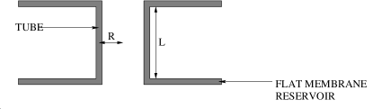
Figure 2: Vertical cross section through idealised tubule configuration showing tubule of length $L$ and radius $R$ bridging two flat bilayers

In this paper we concentrate on the Casimir force acting on the tube described above and shown in Figure 2 in which the electrolyte densities, and hence the Debye masses, are zero in all three layers, the membrane is of fixed thickness $\delta$ with dielectric constant $\epsilon_{2}=\epsilon_{M}=2\epsilon_{vac}$, and the inner and outer layers are filled with water so that $\epsilon_{0}=\epsilon_{3}=\epsilon_{W}=80\epsilon_{vac}$. The Casimir force is thus due purely to the discontinuity in the dielectric constants at the membrane surfaces and is a function of the radius $R$ of the inner cylindrical layer. We shall show that the Casimir force in this case is attractive, tending to collapse the tube. The tube is of length $L$ which we assume is large on any relevant scale, and that there is a reservoir of membrane so that the tube radius $R$ can change without the membrane needing to stretch. For example, the system can be thought of as made from a flat sheet of membrane on to which the tube connects and which acts as a reservoir of membrane as the tube expands or contracts as shown in Figure (2). Alternatively, the membrane can be folded at one end of the tube and act as a reservoir. Both scenarios are possible in biological systems where the membrane is a lipid bilayer, although for the latter it is difficult to calculate the free energy of a given volume of lipid in the reservoir so presents a problem of normalisation. However, it should be emphasised that this picture may nevertheless be an important feature of the stability of lipid tubules and needs further analysis. In either case, because we assume that the membrane is not stretched as the area of the tube increases, there is no elastic energy stored in the tube except that due to the curvature and the surface area of the system is constant. In what follows we shall assume a reservoir of flat membrane as shown in Figure (2).

As an intermediate step we define the grand partition function, $\Xi^{(0)}_{MW}(R,\delta)$, for the membrane normalised by that of an equivalent water filled region, and its associated free energy $F^{(0)}_{MW}(R,\delta)$ by

$$\Xi^{(0)}_{MW}(R,\delta)~{}=~{}\frac{\Xi^{(0)}_{M}(R,\delta)}{\Xi^{(0)}_{W}(R=\infty,\delta)}\;,~{}~{}~{}~{}F^{(0)}_{MW}(R,\delta)~{}=~{}-k_{B}T\log\Xi^{(0)}_{MW}(R,\delta)\;,$$ (73)

where $\Xi^{(0)}_{M}$ is given by Eq. (71), and where $\Xi^{(0)}_{W}$ is the grand partition function of a system filled with water only: $\Xi^{(0)}_{W}=\Xi^{(0)}_{M}$ for $\delta=0$. For the grand ensemble with a reservoir consisting of a flat membrane of the same thickness, shown in Figure 1, we must subtract the free energy of a flat membrane of equivalent area to the tube. We then find that the free energy appropriate to calculate the Casimir force due to the tube geometry is

$$F_{C}(R,\delta)~{}=~{}F^{(0)}_{MW}(R,\delta)~{}-~{}2\pi RL\,F_{\infty}(\delta)\;,$$ (74)

where

$$F_{\infty}(\delta)~{}=~{}\lim_{R\to\infty}\frac{F^{(0)}_{MW}(R,\delta)}{2\pi RL}\;,$$ (75)

where $F_{\infty}(\delta)$ is the free energy per unit area of flat membrane of thickness $\delta$. Using the expression for $\Xi^{(0)}_{M}(R,\delta)$ in Eq. (71) and the asymptotic expressions for $K^{(0)}$ as $r\to 0$ in Eqs. (64) and (65) it can be seen that the dependence on $c_{0}({\bf s})~{}$, which are the coefficients determining the boundary field value $\phi_{0}({\bf x})$ at $r=0$, cancels out $\;\forall{\bf s}\;$ between numerator and denominator in Eq. (73). This is independent of whether the integrals over the $c_{0}({\bf s})$ are done or not; it is a consequence only of separability in the limit $r\to 0$ or, in the case $n=0$, that $K^{(0)}$ becomes independent of the $c_{0}({\bf s})$. Thus we may set $c_{0}({\bf s})=0~{}~{}\forall{\bf s}$ in what follows and omit the integrals over the $c_{0}({\bf s})$.

The difference between the numerator and denominator in $\Xi^{(0)}_{MW}(R,\delta)$ in Eq. (73 is then due to the different contributions of the membrane layer between radii $r_{1}=R-\delta/2$ and $r_{2}=R+\delta/2$ which has dielectric constant $\epsilon_{M}$ in the numerator but $\epsilon_{W}$ in the denominator. We then have

$$\Xi^{(0)}_{MW}(R,\delta)=\int\prod_{\bf s}dc_{1}({\bf s})dc_{2}({\bf s})\;Q^{(0)}({\bf s},c_{2}({\bf s}),r_{2};,c_{1}({\bf s}),r_{1})\>K^{(0)}_{1}({\bf s},c_{2}({\bf s}),r_{2};,c_{1}({\bf s}),r_{1}),$$ (76)

where

$$Q^{(0)}({\bf s},c_{2},r_{2};,c_{1},r_{1})=\lim_{{r_{3}\to\infty}\atop{r_{0}\to 0}}\frac{K_{0}({\bf s},0,r_{3};c_{2},r_{2})K_{2}({\bf s},c_{1},r_{1};0,r_{0})}{K({\bf s},0,r_{3};0,r_{0})}\;,$$ (77)

where in $Q^{(0)}$ the dielectric constant in the denominator kernel is $\epsilon_{W}$. From the asymptotic expressions in Eqs. (56-67) we find that $Q^{(0)}$ has a simple form for $(n,p)\neq(0,0)$ ( c.f. ${\bf s}=(n,p)$)

$$Q^{(0)}({\bf s},c_{2},r_{2};,c_{1},r_{1})$$ (78)

$$= \left[\frac{{\beta\epsilon}_{W}}{2\pi|K_{n}(pr_{2})I_{n}(pr_{1})|}\right]^{1/2}\exp\left(\frac{-{\beta\epsilon}_{W}}{2}V_{n}(pr_{2})c_{2}^{2}\right)\>\exp\left(-\frac{{\beta\epsilon}_{W}}{2}U_{n}(pr_{1})c_{1}^{2}\right)\;,$$

where $U_{n},V_{n}$ are defined in Eqs. (66) and (59), respectively. Note, that all Debye masses are zero here. For large argument $U_{n},V_{n}\to 1$, and so both Gaussian forms are convergent and integrable. $Q^{(0)}$ takes the form of a normalised product of a generalisation of harmonic oscillator ground state wave-functions in $c_{1}$ and $c_{2}$, and satisfies the appropriate Schrödinger equations in these variables. For large $R$ and $n>0$ these functions become the usual ground-state oscillator wave-functions with $m\omega={\beta\epsilon}_{W}n$, which agrees with the analysis of the planar film of [4].

For $(n,p)=(0,0)$ we find

$$Q^{(0)}({\bf s}=\mbox{\boldmath$0$},c_{2},r_{2};,c_{1},r_{1})~{}=~{}\lim_{{r_{3}\to\infty}\atop{r_{0}\to 0}}\left[\frac{{\beta\epsilon}_{W}}{2\pi}\frac{t_{30}}{t_{32}t_{10}}\right]^{1/2}\exp\left(-\frac{{\beta\epsilon}_{W}}{2}\frac{c_{2}^{2}}{t_{32}}\right)\exp\left(-\frac{{\beta\epsilon}_{W}}{2}\frac{c_{1}^{2}}{t_{10}}\right),$$ (79)

where $t_{i}=\log r_{i}$ and $t_{ij}=t_{i}-t_{j}$. Also, we have that

$$K^{(0)}_{1}({\bf s}=\mbox{\boldmath$0$},c_{2}({\bf s}),r_{2};,c_{1}({\bf s}),r_{1})~{}=~{}\left[\frac{{\beta\epsilon}_{M}}{2\pi}\frac{1}{t_{21}}\right]^{1/2}\exp\left(-\frac{{\beta\epsilon}_{W}}{2}\frac{(c_{1}-c_{2})^{2}}{t_{21}}\right)\;,$$ (80)

and so we find the contribution from ${\bf s}=\mbox{\boldmath$0$}$ mode to the partition function is

$$\Xi^{(0)}_{MW}({\bf s}=\mbox{\boldmath$0$},R,\delta)~{}=~{}~{}\lim_{{r_{3}\to\infty}\atop{r_{0}\to 0}}\left[\frac{\epsilon_{W}\epsilon_{M}t_{30}}{\epsilon_{W}(\epsilon_{W}-\epsilon_{M})t_{21}+{\epsilon_{W}\epsilon_{M}}t_{30}}\right]^{1/2}~{}=~{}1\;.$$ (81)

Thus, the zero mode does not contribute to the free energy of the membrane. However, it is the relevant mode to show that the charge neutrality condition holds. The total charge operator $\Sigma$ is given by

$$\Sigma~{}=~{}\epsilon_{W}\int d{\bf x}E({\bf x},r_{2}+\eta)-\epsilon_{W}\int d{\bf x}E({\bf x},r_{1}-\eta)\;,$$ (82)

where $E({\bf x},r)$ is the radial component of the electric field and $\eta$ is a small positive length; thus, we measure the field in the water just outside the membrane surfaces. We have that

$$E({\bf x},t)~{}=~{}-\frac{\partial}{\partial r}\langle\phi({\bf x},r)\rangle~{}=~{}-\frac{1}{J(t)}\langle\frac{\partial}{\partial t}\phi({\bf x},t)\rangle~{}=~{}-\frac{1}{J(r(t){\beta\epsilon}_{W}}\langle\pi({\bf x},t)\rangle\;,$$ (83)

now considering $E$ and $\phi$ as functions of $t=\log(r)$. Here $\pi({\bf x},t)$ is the momentum operator conjugate to $\phi({\bf x},t)$ and is given by $\pi({\bf x},t)={\beta\epsilon}\dot{\phi}({\bf x},t)$ using standard theory. The Schrödinger representation of $\pi({\bf x},t)$ [22] then gives

$$E({\bf x},t)~{}=~{}\frac{1}{J(t){\beta\epsilon}}\langle\phi,t|\;\frac{\delta}{\delta\phi({\bf x})}\;|\phi,t\rangle\;.$$ (84)

The contribution to $\langle\Sigma\rangle$ from the integral over the surface at $r=r_{1}$ is then

$$\langle\Sigma_{1}\rangle~{}=~{}\frac{1}{J(t)\beta}\langle{\tilde{\phi}},t|\;\frac{\delta}{\delta{\tilde{\phi}}(\mbox{\boldmath$0$})}\;|{\tilde{\phi}},t\rangle\;,$$ (85)

where ${\tilde{\phi}}(\mbox{\boldmath$0$})$ is the zero-mode field. Using Eqs. (57) and (79) we then find

$$\langle\Sigma_{1}\rangle~{}=~{}\lim_{t_{0}\to-\infty}\frac{\epsilon_{W}}{J(t_{1})}\frac{\langle{\tilde{\phi}},t_{1}|\;{\tilde{\phi}}(\mbox{\boldmath$0$})\;|{\tilde{\phi}},t_{1}\rangle}{t_{1}-t_{0}}~{}=~{}0\;.$$ (86)

A similar result holds for $\langle\Sigma_{2}\rangle$, the contribution to $\langle\Sigma\rangle$ from the surface integral at $r=r_{2}$; thus we find that $\langle\Sigma\rangle=0$. This analysis can be repeated to show that all moments of $\Sigma$ vanish: $\langle\Sigma^{n}\rangle=0,~{}\forall n>0$; it is this condition that ensures charge neutrality of the system.

We now calculate the free energy $F^{(0)}$ by summing over all ${\bf s}=(n,p)$ mode contributions. From the previous section we find

$$K^{(0)}_{1}({\bf s},c_{2}({\bf s}),r_{2};,c_{1}({\bf s}),r_{1})$$

$$\hbox to0.0pt{\hss${}={}$}\left[\frac{{\beta\epsilon}_{M}}{2\pi|H_{n}(pr_{2},pr_{1})|}\right]^{1/2}\exp\left(-\frac{{\beta\epsilon}_{M}}{2}{\mbox{\boldmath$c$}}({\bf s})\cdot\mbox{\boldmath$D$}({\bf s},r_{2},r_{1})\cdot{\mbox{\boldmath$c$}}({\bf s})\right),$$ (87)

where as before ${\mbox{\boldmath$c$}}=(c_{1},c_{2})$ and

$$\mbox{\boldmath$D$}({\bf s},r_{2},r_{1})~{}=~{}\frac{1}{H_{n}(pr_{2},pr_{1})}\left(\begin{array}[]{cc}W_{n}(pr_{2},pr_{1})&1\\ &\\ 1&W_{n}(pr_{1},pr_{2})\end{array}\right)\;,$$ (88)

and $W_{n}$ and $H_{n}$ are defined in Eq. (54). Using Eqs. (76), (78), and (87) we find

$$\Xi^{(0)}_{MW}(R,\delta) =$$

$$\int\prod_{\bf s}\frac{1}{2\pi} dc_{1} ({\bf s})dc_{2}({\bf s})\left[\frac{{\beta\epsilon}_{W}}{|K_{n}(pr_{2})I_{n}(pr_{1})|}\right]^{1/2}\left[\frac{{\beta\epsilon}_{M}}{|H_{n}(pr_{2},pr_{1})|}\right]^{1/2}$$ (89)

$$\exp\left(-\frac{\beta}{2}{\mbox{\boldmath$c$}}({\bf s})\cdot\mbox{\boldmath$E$}_{M}({\bf s},r_{2},r_{1})\cdot{\mbox{\boldmath$c$}}({\bf s})\right)\;,$$

where

$$\mbox{\boldmath$E$}_{M}({\bf s},r_{2},r_{1})~{}=~{}\epsilon_{M}\mbox{\boldmath$D$}({\bf s},r_{2},r_{1})+\epsilon_{W}\mbox{\boldmath$X$}({\bf s},r_{2},r_{1})\;,$$ (90)

and

$$\mbox{\boldmath$X$}({\bf s},r_{2},r_{1})=\mbox{diag}[U_{n}(pr_{1}),\;V_{n}(pr_{2})]\;,$$ (91)

is a $2\times 2$ diagonal matrix. A more useful alternative expression is

$$\Xi^{(0)}_{MW}(R,\delta)~{}=~{}\left(\frac{\epsilon_{M}}{\epsilon_{W}}\right)^{1/2}\prod_{\bf s}\frac{\displaystyle\int d{\mbox{\boldmath$c$}}({\bf s})\exp\left(-\frac{\beta}{2}{\mbox{\boldmath$c$}}({\bf s})\cdot\mbox{\boldmath$E$}_{M}({\bf s},r_{2},r_{1})\cdot{\mbox{\boldmath$c$}}({\bf s})\right)}{\displaystyle\int d{\mbox{\boldmath$c$}}({\bf s})\exp\left(-\frac{\beta}{2}{\mbox{\boldmath$c$}}({\bf s})\cdot\mbox{\boldmath$E$}_{W}({\bf s},r_{2},r_{1})\cdot{\mbox{\boldmath$c$}}({\bf s})\right)}\;,$$ (92)

where

$$\mbox{\boldmath$E$}_{W}({\bf s},r_{2},r_{1})~{}=~{}\epsilon_{W}(\mbox{\boldmath$D$}({\bf s},r_{2},r_{1})+\mbox{\boldmath$X$}({\bf s},r_{2},r_{1}))\;.$$ (93)

The denominator is the contribution from a pure water-filled system. The two expressions for $\Xi^{(0)}_{MW}(R,\delta)$ are the same since using the Wronskian identity, Eq. (24), we find

$$\det[\mbox{\boldmath$D$}({\bf s},r_{2},r_{1})+\mbox{\boldmath$X$}({\bf s},r_{2},r_{1})]~{}=~{}-[K_{n}(pr_{2})I_{n}(pr_{1})H_{n}(pr_{2},pr_{1})]^{-1}.$$ (94)

Then we have

$$\Xi^{(0)}_{MW}(R,\delta) = \frac{1}{2}\left(\frac{\epsilon_{M}}{\epsilon_{W}}\right)^{1/2}\prod_{\bf s}\det[\mbox{\boldmath$B$}({\bf s},r_{2},r_{1})]\;,$$

$$\mbox{\boldmath$B$}({\bf s},r_{2},r_{1}) = \left[1+(\mbox{\boldmath$X$}({\bf s},r_{2},r_{1})+\mbox{\boldmath$D$}({\bf s},r_{2},r_{1}))^{-1}\mbox{\boldmath$X$}({\bf s},r_{2},r_{1})\frac{(\epsilon_{W}-\epsilon_{M})}{\epsilon_{M}}\right]\;,$$ (95)

and the total free energy of the tube is

$$F_{C}(R,\delta) = F^{(0)}_{MW}(R,\delta)-F^{(0)}_{f}(\delta)\;,$$

$$F^{(0)}_{MW}(R,\delta) = -{\textstyle{1\over 2}}k_{B}T\log\left(\frac{\epsilon_{M}}{4\epsilon_{W}}\right)+L\sum_{n}\int\frac{dp}{2\pi}\;F^{(0)}_{MW}({\bf s},R,\delta)\;,$$

$$F^{(0)}_{MW}({\bf s},R,\delta) = -k_{B}T\log(\det[\mbox{\boldmath$B$}({\bf s},r_{2},r_{1})])\;.$$ (96)

The required free energy $F_{C}(R,\delta)$ is then given by Eqs. (73) and (74). Using Eqs. (52) and (46) it can be verified, as expected, that $F^{(0)}_{MW}(R,\delta=0)=0$. From Eq. (92) we find also that $F^{(0)}_{MW}(R,\delta)=0$ when $\epsilon_{W}=\epsilon_{M}$ .

6 Evaluation of the Casimir energy

In this section we evaluate the Casimir energy for the dielectric tube as a function of the inner radius $R$ formed from a membrane of fixed thickness $\delta$ and dielectric constant $\epsilon_{M}$. The regions interior and exterior to the tube are water-filled with dielectric constant $\epsilon_{W}$. The cross-section of the tube is shown in Figure 2 and the length of the tube is aligned along the $z$-axis.

The result for the free energy of the tube, $F_{C}(R,\delta)$, is given in Eqs. (96) as a sum over the mode number $n$ and an integral over the wave-vector, $p$, in the $z$-direction. We evaluate the sum and integral numerically and present results in the next section for various values of $\delta$. However, as is usual in many cases, the calculation is dominated by the Ultra-Violet (UV) properties of the integrand and an UV cut-off must be imposed to achieve a finite result. We examine the UV properties of the integral and calculate the leading divergent contributions analytically. These divergent contributions, which are regulated by the UV cut-off, agree with the prediction for them obtained from the full numerical calculation. We also verify that the $R\to\infty$ limit of $F^{(0)}_{MW}(R,\delta)$ agrees with the result in the planar film case for a film of thickness $\delta$. It is convenient to define the following constants which encode the dielectric properties of the system

$$\Delta=\frac{\epsilon_{W}-\epsilon_{M}}{\epsilon_{W}+\epsilon_{M}}\;,~{}~{}~{}~{}\gamma=\frac{\epsilon_{W}}{\epsilon_{M}}-1~{}=~{}\frac{2\Delta}{1-\Delta}\;.$$ (97)

After some algebra and use of the Wronskian identity Eq. (52) we find

$$(\mbox{\boldmath$D$}({\bf s},r_{2},r_{1})+\mbox{\boldmath$X$}({\bf s},r_{2},r_{1}))^{-1}~{}=~{}\left(\begin{array}[]{cc}I_{n}(pr_{1})K_{n}(pr_{1})&I_{n}(pr_{1})K_{n}(pr_{2})\\ &\\ I_{n}(pr_{1})K_{n}(pr_{2})&I_{n}(pr_{2})K_{n}(pr_{2})\end{array}\right).$$ (98)

Using the expression for the diagonal matrix $X$ in Eq. (91) we find that $\mbox{\boldmath$B$}({\bf s},r_{2},r_{1})$, whose determinant is required for the evaluation of $\Xi^{(0)}$ in Eq. (95), is

$$\mbox{\boldmath$B$}({\bf s},r_{2},r_{1})~{}=~{}\left(\begin{array}[]{cc}1+\gamma I^{\prime}_{n}(pr_{1})K_{n}(pr_{1})&-I_{n}(pr_{1})K^{\prime}_{n}(pr_{2})\\ &\\ I^{\prime}_{n}(pr_{1})K_{n}(pr_{2})&1-\gamma I_{n}(pr_{2})K^{\prime}_{n}(pr_{2})\end{array}\right)\;.$$ (99)

The important feature of $B$ is that the on-diagonal elements are the separate contributions from the surfaces at $r=r_{1}$ and $r=r_{2}$ and the off-diagonal terms are the contribution from the interaction between the surfaces. In particular, it will be shown later in this section that the off-diagonal elements fall off exponentially with the surface separation $\delta$ like $\exp(-2\sqrt{(}p^{2}+m^{2})\delta)$. This fact has the consequences that the inter-surface interaction becomes negligible for large separations or for large wave-vector $p$. The corollary is that any Ultra-Violet divergences, which are due to large $p$ behaviour of the integrand, arise solely from the separate surface contributions and that the inter-surface interaction gives a UV-finite contribution. We therefore explicitly separate the terms in $F^{(0)}_{MW}(R,\delta)$ into these respective contributions. We have

$$\frac{F^{(0)}_{MW}(R,\delta)}{Lk_{B}T}~{}=~{}\frac{1}{r_{1}}g(\Lambda r_{1},\Delta)+\frac{1}{r_{2}}g(\Lambda r_{2},-\Delta)+h(r_{1},r_{2},\Lambda,\Delta)+m(\Lambda,\Delta)\;,$$ (100)

where

$$g(x,\Delta)~{} =~{}\frac{1}{2\pi}\sum_{n}\int_{0}^{x}du\log[1+\Delta(I_{n}(u)K_{n}(u))^{\prime}]\;,$$

$$h(r_{1},r_{2},\Lambda,\Delta)~{} =~{}$$

$$\frac{1}{2}\int_{0}^{\Lambda}\frac{dk}{\pi}\sum_{n} \log\left[1+\frac{\displaystyle 4\Delta^{2}p^{2}r_{1}r_{2}I^{\prime}_{n}(pr_{1})I_{n}(pr_{1})K^{\prime}_{n}(pr_{2})K_{n}(pr_{2})}{\displaystyle(1+\Delta pr_{1}(I_{n}(pr_{1})K_{n}(pr_{1})^{\prime})((1-\Delta pr_{2}(I_{n}(pr_{2})K_{n}(pr_{2})^{\prime})}\right]\;,$$

$$m(\Lambda,\Delta)~{} =~{}-\frac{1}{2}\int_{0}^{\Lambda}\frac{dk}{\pi}\sum_{n}\log(1-\Delta^{2})\;.$$ (101)

The contribution $Lk_{B}Tg(\Lambda r,\Delta)/R$ is the free energy of an isolated cylinder of length $L$, radius $R$ and dielectric constant $\epsilon_{M}$ in a medium of dielectric constant $\epsilon_{W}$. Thus the first two terms in Eq. (100) are the respective separate contributions of the inner and outer cylindrical regions that form the layer of thickness $\delta=r_{2}-r_{1}$; the term $Lk_{B}Th(r_{1},r_{2},\Lambda,\Delta)$ is the contribution from the interaction between the cylinders. As expected, the function $g(x,\Delta)$ diverges as $x\to\infty$ and so this term in the free energy must be regulated by taking a finite non-zero cut-off $\Lambda=\pi/a$, where $a$ is the UV cut-off length. Viewed as a Taylor expansion in $\Delta$ we find that the $O(\Delta)$ term of $g$ is independent of $r$ and so in the free energy the contributions proportional to $\Delta$ cancel. This to be expected on physical grounds since by examining the limit of a diffuse system one can see that any term proportional to $\Delta$ must be a self energy term [25]. The term of order $\Delta^{2}$ of $g$ can be evaluated using Bessel function summation theorems [24]. This term is given by

$$g_{2}(x,\Delta)~{}=~{}-\frac{\Delta^{2}}{4\pi}\int_{0}^{x}du\;u^{2}\sum_{n}{[I_{n}(u)K_{n}(u)]^{\prime}}^{2}\;.$$ (102)

We define $R^{*}(r_{1},r_{2},\phi)=\sqrt{r_{1}^{2}+r_{2}^{2}-2r_{1}r_{2}\;\hbox{cos}(\phi)}~{}$ and from [24] we have

$$K_{0}(uR^{*}(r_{1},r_{2},\phi))~{}=~{}\sum_{n}I_{n}(ur_{1})K_{n}(ur_{2})e^{in\phi}\;.$$ (103)

Then

$$K_{0}(2uR^{*}(1,1,\phi)) = \sum_{n}I_{n}(u)K_{n}(u)\;e^{in\phi}~{}~{}~{}~{}\Longrightarrow$$

$$2\;\hbox{sin}(\phi/2)\,K_{0}^{\prime}(2u\;\hbox{sin}(\phi/2)) = \sum_{n}\;[I_{n}(u)K_{n}(u)]^{\prime}\;e^{in\phi}\;.$$ (104)

Thus

$$\sum_{n}{[I_{n}(u)K_{n}(u)]^{\prime}}^{2}~{}=~{}\frac{2}{\pi}\int_{0}^{2\pi}K_{1}^{2}(2u\;\hbox{sin}(\phi/2))\;\hbox{sin}^{2}(\phi/2)\;,$$ (105)

where the Bessel function identity $K_{0}^{\prime}(u)=-K_{1}(u)$ has been used. By substitution into Eq. (102) and careful manipulation of the double integral we find that

$$g(x,\Delta)~{}=~{}-\frac{1}{256}\Delta^{2}\left[6\log(x)+30\log 2+6\gamma-11\right]~{}+~{}O(\Delta^{4})+O(1/x)\;.$$ (106)

Similarly, the finite contribution $h(r_{1},r_{2},\Lambda,\Delta)$ can be expanded and the $O(\Delta^{2})$ term evaluated. We have

$$h_{2}(r_{1},r_{2},\Lambda,\Delta)~{}=~{}\frac{2}{\pi}\Delta^{2}\int_{0}^{\Lambda}dp\;r_{1}r_{2}\sum_{n}\;p^{2}I^{\prime}_{n}(pr_{1})I_{n}(pr_{1})K^{\prime}_{n}(pr_{2})K_{n}(pr_{2})\;.$$ (107)

Using Eq. (103) we have

$$\sum_{n}p^{2}I^{\prime}_{n}(pr_{1})I_{n}(pr_{1})K^{\prime}_{n}(pr_{2})K_{n}(pr_{2})$$

$$\hbox to0.0pt{\hss${}={}$}\frac{1}{2\pi}\int_{0}^{2\pi}d\phi\;\frac{\partial K_{0}}{\partial r_{1}}(pR^{*}(r_{1},r_{2},\phi))\frac{\partial K_{0}}{\partial r_{2}}(pR^{*}(r_{1},r_{2},\phi))\;.$$ (108)

Because the integral is convergent we may set $\Lambda$ to $\infty$. We find

$$h_{2}(r_{1},r_{2},\Lambda,\Delta)$$

$$\hbox to0.0pt{\hss${}={}$}\frac{\Delta^{2}r_{1}r_{2}}{\pi}\int_{0}^{\infty}du\;K_{1}(u)^{2}\;\int_{0}^{2\pi}d\phi\;\frac{(r_{1}-r_{2}\;\hbox{cos}(\phi))(r_{2}-r_{1}\;\hbox{cos}(\phi))}{(r_{1}^{2}+r_{2}^{2}-2r_{1}r_{2}\;\hbox{cos}(\phi))^{5/2}}\;,$$ (109)

with $r_{1}=R-\delta/2,~{}r_{2}=R+\delta/2$. After manipulation we find that

$$h_{2}(r_{1},r_{2},\Lambda,\Delta)~{}=~{}\frac{3}{64}\frac{\Delta^{2}}{R}\frac{1-y^{2}}{y^{2}}\int_{0}^{\infty}dz\;\frac{y^{2}z^{4}-1}{(1+y^{2}z^{2})^{1/2}(1+z^{2})^{5/2}}\;,$$ (110)

where $y=\delta/2R$. This gives

$$h_{2}(r_{1},r_{2},\Lambda,\Delta)~{}=~{}\frac{\Delta^{2}}{2\delta^{2}}~{}+~{}\frac{3}{64}\frac{\Delta^{2}}{R}\left[\log\left(\frac{\delta}{2R}\right)+2\log 2-\frac{1}{2}\right]\;.$$ (111)

6.1 $R\to\infty,$ $\delta$ fixed

To calculate $F_{C}(R,\delta)$ in the grand canonical ensemble we must subtract from $F^{(0)}_{MW}(R,\delta)$ the free energy $F_{\infty}$, defined in Eq. (75), for a flat membrane of the same area and thickness. This has been calculated in previous work [4] but is it instructive to derive it directly from Eq. (100). In the limit $R\to\infty$ the arguments of all functions for $p\neq 0$ become large and we find that the calculation is dominated by large $n$. The leading asymptotic results given in Eq. (123) will be sufficient to compute $F^{(0)}_{MW}({\bf s},R,\delta)$ in the large $R$ limit.

From Eq. (123) we have for large $n$ that

$$I_{n}(pr) \sim \frac{1}{\sqrt{2\pi}}\frac{1}{(n^{2}+p^{2}r^{2})^{1/4}}\>\exp\big{[}n\eta(pr/n)\big{]}\;,$$

$$K_{n}(pr) \sim \sqrt{\frac{\pi}{2}}\frac{1}{(n^{2}+p^{2}r^{2})^{1/4}}\>\exp\big{[}-n\eta(pr/n)\big{]}\;,$$

$$I_{n}^{\prime}(pr) \sim \sqrt{\frac{1}{2\pi}}\frac{(n^{2}+p^{2}r^{2})^{1/4}}{pr}\>\exp\big{[}n\eta(pr/n)\big{]}\;,$$

$$K_{n}^{\prime}(pr) \sim -\sqrt{\frac{\pi}{2}}\frac{(n^{2}+p^{2}r^{2})^{1/4}}{pr}\>\exp\big{[}-n\eta(pr/n)\big{]}\;.$$ (112)

In the limit $R\to\infty$ it is better to define a new two-dimensional wave-vector ${\bf k}=(n/R,p)$ (i.e., $k_{1}=n/R,~{}k_{2}=p$), since we then find that the $R\to\infty$ limit can be formulated in terms of functions with finite arguments. The measure is then

$$L\sum_{n}\int\frac{dp}{2\pi}~{}\to~{}2\pi LR\int\frac{d^{2}k}{(2\pi)^{2}}\;.$$ (113)

Note that $A=2\pi LR$ is the area of the tube.

From Eq. (112) and using the definition of $\eta(z)$ in Eq. (124) we obtain

$$\eta\left(\frac{p}{n}(R+\delta/2)\right)-\eta\left(\frac{p}{n}(R-\delta/2)\right)~{}\sim~{}k_{2}\delta\>\eta^{\prime}\left(k_{2}/k_{1}\right)~{}=~{}(k_{1}^{2}+k_{2}^{2})^{1/2}\delta~{}\equiv~{}k\delta\;.$$ (114)

The next correction is $O(\delta^{3}/R^{2})$ which is negligible in the $R\to\infty$ limit. Then we find

$$(I_{n}(pr_{1})K_{n}(pr_{1}))^{\prime} \sim (I_{n}(pr_{2})K_{n}(pr_{2}))^{\prime}~{}\sim~{}0\;,$$ (115)

$$I_{n}^{\prime}(pr_{1})I_{n}(pr_{2})K_{n}(pr_{1})K_{n}^{\prime}(pr_{2}) \sim -\frac{1}{4p^{2}r_{1}r_{2}}\exp(-2k\delta)\;.$$ (116)

Using Eq. (115), we see immediately that the contributions from the individual surfaces vanish in this limit. The non-zero contributions then arise only from $h(r_{1},r_{2},\Lambda,\Delta)$ and trivially from $m(\Lambda,\Delta)$ in Eq. (101). On substitution in to Eq. (100) we find in the large $R$ limit that

$$\beta F_{\infty}(\delta)~{}=~{}-\frac{1}{2}\int\frac{d^{2}k}{(2\pi)^{2}}\;\Bigg{[}\log\Big{(}1-\Delta^{2}\Big{)}~{}-~{}\log\Big{(}1-\Delta^{2}\exp(-2k\delta)\Big{)}\Bigg{]}\;.$$ (117)

We consider this result in the limit $\delta\to 0$. The integral in Eq. (117) must be regulated with a UV cutoff $k\leq\Lambda$. The second logarithm in this equation can be expanded and the series in $\Delta^{2}$ integrated term by term. If we assume that $\Lambda\delta\gg 0$ then we find

$$\beta F_{\infty}(\delta)~{}=~{}-\frac{A}{8\pi}\Bigg{[}\frac{\Lambda^{2}}{4}\log\Big{(}1-\Delta^{2}\Big{)}~{}-~{}\frac{1}{2\delta^{2}}\sum_{m}\frac{\Delta^{2m}}{m^{3}}\Bigg{]}\;.$$ (118)

The result behaves like $1/\delta^{2}$ but only as long as the assumption $\Lambda\delta\gg 0$ holds since terms containing the factor $\exp(-\Lambda\delta)$ have been ignored. If all terms are kept then, of course, $\lim_{\delta\to 0}F_{\infty}(\delta)=0$.

On subtracting $2\pi RLk_{B}TF_{\infty}$ from $F^{(0)}_{MW}$ to obtain the grand free energy $F_{C}$ we see that the first term in $F_{\infty}$ cancels the contribution from $m(\Lambda,\Delta)$ in Eq. (100) identically. We retain the second term in $F_{\infty}$ at $O(\Delta^{2})$ and it cancels a similar term in the evaluation of the integral for $h_{2}(r_{1},r_{2},\Lambda,\Delta)$. This term is exhibited explicitly in Eq. (111). Putting our results together we find that $\kappa_{C}$ defined in Eq. (4) is given by

$$\kappa_{C}~{}=~{}\frac{\Delta^{2}}{64}\left[3\log\left(\frac{\pi\delta}{a}\right)+6\log 2+3\gamma_{E}-4\right]+\Delta^{4}B(\Delta)\;,$$ (119)

where $\gamma_{E}$ is Euler’s constant and the constant in the brackets is evaluated to be $0.02954\ldots$. We note an important point which is that the $\log(R)$ dependences from the functions $g$ and $h$ cancel exactly giving a leading order behaviours of $F_{C}\sim 1/R$.

7 Numerical Results

In order to calculate the Casimir energy as a function of $R$ and $\delta$ we evaluate $F_{C}(R,\delta)$, defined in Eqs. (96) and (100), numerically. The free energy $F_{C}(R,\delta)$ is normalised to zero for $R=\infty$, and is defined in terms of the free energy $F^{(0)}_{MW}(R,\delta)$ which is normalised to be zero when the dielectric constant of the membrane, $\epsilon_{M}$ is set equal to that for water: $\epsilon_{M}=\epsilon_{W}$. Here, $F^{(0)}_{MW}(R,\delta)$ is given as a sum over $n$ and integral over $p$ of $F^{(0)}_{MW}({\bf s},R,\delta)$ (${\bf s}=(n,p)$), itself defined in Eq. (96).

To carry out both the sum over $n$ and the integral over $p$ we use the VEGAS integration package [26] which is an efficient algorithm which uses importance sampling to do multidimensional integrals. Although we are dealing with a discrete sum over $n$ it is easy to adapt the integrand so that it is a function of the continuous variable $x$ through the relation

$$n(x)~{}=~{}R\;\mbox{Int}(\hat{x})\;,~{}~{}~{}~{}\hat{x}~{}=~{}x-0.5(1-\hbox{sign}(x))\;.$$ (120)

Then $n(x)$ takes integer values necessary for the summation whilst $x$ is used as a continuous integration variable by VEGAS. Both the sum over $n$ and the integral over $p$ are done by efficient importance sampling techniques, and an accurate answer can be obtained. To impose the needed Ultra-Violet regulator or cut-off, we set ${\bf k}=(n(x)/R,\;p)$ and integrate over the region $-\pi/a\leq k\leq-\pi/a\;,~{}~{}k=|{\bf k}|$.

The evaluation of the integrand poses some difficulties since, as we have seen in the previous section, the integrand is dominated by large values of $k$, and hence the arguments of the Bessel functions in the definition of $F^{(0)}_{MW}({\bf s},R,\delta)$, Eqs. (100) and (101), become very large indeed. In this case the function $I_{n}$ ($K_{n}$) suffers from floating point overflow (underflow), which can be seen easily from the asymptotic forms given in Eq. (123). However, in contrast the products over the Bessel functions which constitute each term in Eq. (101) do not suffer in this way. This also can be seen from Eq. (116) where the increasing and decreasing exponential behaviours of $I_{n}$ and $K_{n}$, respectively, compensate to give the behaviours $\exp(-2k\delta)$. To construct a robust integrand we used routines for the full Bessel functions when $k$ was sufficiently small and used the appropriate asymptotic form given in (123) when either $n$ or $p$, or both, became large. It was then possible to cancel the diverging and vanishing exponential factors against each other, so obtaining a well defined integrand computationally.

We take $\epsilon_{W}/\epsilon_{M}=40$ and evaluate $F_{C}(R,\delta)$ as a function of $R$ in nanometers, and $\delta=5(nm),~{}10(nm)$ and for various values of the cutoff length $a$. Because there is no electrolyte the temperature dependence is purely in the factor of $k_{B}T$ multiplying our calculation. From Eq. (119) it is clear that, as is true in most applications, the Casimir energy is dominated by the UV cutoff behaviour and hence by the value chosen for $a$. It is not fully clear what the correct value for $a$ should be since the microscopic properties of the membrane interface are not properly included in the analysis. Typically, we would expect $a$ to be the scale of the inter-molecular spacing of the molecules forming the membrane or of water molecules. For this calculation a reasonable value is $a\sim 0.5(nm)$. To test the validity of our UV analysis we first investigate how $F_{C}(R,\delta)$ behaves for very small $a$ and we choose $a=0.05,~{}0.1,~{}0.2,~{}0.5(nm)$. The function $B(\Delta^{2})$ receives contribution from the both the $g$ and $h$ terms in Eq. (27) with $B(0)\neq 0$. Note that there are no odd terms in $\Delta$ in the leading $1/R$ behaviour of $F_{C}$ since to leading order one may set $\delta/R=0$ (equivalently $R_{1}=R_{2}$) in the leading order behaviour of $g$ and in the denominator of the second term in the logarithm of the integral defining $h$. This is a consistent parametrisation whilst $\delta\gg a$. The limit $\delta\to 0$ must be taken carefully and when $\delta<a$ the separation of $F^{(0)}_{MW}$ in Eq. (100) into contributions from functions $g$ and $h$ is not useful since $h$ develops the compensating UV divergence to that in $g$ and we find $\lim_{\delta\to 0}F_{C}=0$, as expected; in essence, the larger of $(\delta,a)$ acts as the $UV$ cut-off on the integral defining $h$.

In Table 1, for various values of $\Delta$ and $\delta/a$, we compare the prediction of Eq. (119) with the result of numerical evaluation and deduce a numerical value for $B(\Delta^{2})$. Owing to small systematic errors in the numerical calculation of the Bessel functions there is a tiny discrepancy for very small $\Delta$ but $B(\Delta^{2})$ is seen to be a constant function from evaluations at larger $\Delta$ and we see that $B(0)$ is plausibly $1/8$.

$\Delta$	$~{}~{}\delta/a$	$O(\Delta^{2})$ coeff. of $1/R$ from Eq. (119)	Coeff. of $1/R$ from simulation	$B(\Delta^{2})$
78/82	$10^{3}$	-0.342	-0.443	0.123
78/82	$10^{2}$	-0.244	-0.346	0.123
0.6	$10^{3}$	-0.1361	-0.1520	0.123
0.6	$10^{2}$	-0.0972	-0.0162	0.123
0.2	$10^{3}$	-0.0151	-0.0162	–
0.6	$10^{3}$	-0.0038	-0.0040	–

Table 1: For various values of $\Delta$ and $\delta/a$ we compare the prediction of Eq. (119) with the result of simulation and deduce a numerical value for $B(\Delta^{2})$. Owing to small systematic errors in the numerical calculation of the Bessel functions there is a negligible discrepancy for very small $\Delta$ but $B(\Delta^{2})$ is seen to be a constant function from evaluations at larger $\Delta$. We see that the result for $F_{C}$ from Eq. (119) is in very good agreement with the full calculation. Various values of $\delta$ and $a$ were used but typically $\delta=1-10$(nm)

The physical value of the UV cut-off length can only be determined phenomenologically in this model. This is because the model is an effective field theory in which the dynamics of the molecular electric dipoles is described by the dielectric constant which is a static long-range parameter. The field modes with large-$k$ and $n$ probe the static short distance properties of the model and so a more refined field theory is needed for these scales. It is unclear whether the molecular nature of the lipid has an effect on the UV cutoff but it would seem most likely that the effective value of $\epsilon_{W}$ at short scales are dominant in this calculation. The effect is encoded in the value of $a$.

8 Conclusion

In this paper we have developed the theory for a general approach to the calculation of the electrostatic free energy for a system of symmetrically layered electrolytic membranes. The definition of symmetrical is that the Laplacian is separable and that the coordinate direction normal to the layers can be interpreted in terms of a Euclidean time variable, $t$. The x partition function for a layer bounded by surfaces defined by $t=t_{i}$ and $t=t_{j},~{}t_{i}<t_{j}$ can then be written in terms of the Feynman (Euclidean) time evolution kernel from $t_{i}$ to $t_{j}$ by invoking the well-known connection between this formalism and statistical mechanics. The method is a general extension of our work concerning flat membranes [4],[27], [22], [8] and allows the full interacting Sine-Gordon field theory in Eq. (7) for electrolytic layers to be studied systematically, including the perturbation theory in the coupling constant $g$ defined by $g=l_{B}/l_{D}$, where $l_{B}$ and $l_{D}$ are the Bjerrum and Debye lengths, respectively. Geometries of interest to which this approach applies include cylindrical and spherical ones. In this paper the general theory developed in section 3 is applied to the system of cylindrical layers each filled with a pure dielectric medium where the dielectric constant differs between layers. The analysis of this system is based on the free harmonic field theory which is exactly soluble and which is the theory about which a perturbative expansion for the effect of fluctuations takes place. In the succeeding sections the particular problem of the free energy of a tube of dielectric material submersed in water is studied and the Casimir force calculated. The tube is a simple model for the t-tubule formed from lipid membrane in particular kinds of muscle cell and the object of the calculation is to investigate the size and form of the Casimir force and whether it can act to stabilise the tube against bending stress that acts to decrease the tube curvature and hence increase its radius. In order to calculate the relevant free energy we assumed that the tube was connected to an infinite reservoir of flat membrane and so worked with the grand ensemble describing this system. The assumption about which ensemble is the relevant one is crucial to answering questions concerning tubule stability since in the grand ensemble the nature of the lipid or membrane reservoir determines its bulk free energy and hence affects the energy of conformation of the tube; a flat membrane reservoir will differ for a reservoir which stores spare lipid at the end of the tubule essentially as crumpled membrane. Clearly also, if there is no reservoir at all, so that the ensemble is canonical, then any increase in the surface area of the tube as it expands will lead to a lower density of lipids in the surface and a concomitant increase in the surface energy over and above that due to the bending stress; this is a fundamentally different situation to the one we assume.

In the case studied here we see from Table 1 that for a lipid bilayer tube in water with $\delta=10$(nm) and $a=0.1$(nm) we find $\kappa_{C}=0.346$. It is possible to include the contributions from the modes with non-zero Matsubara frequencies, a calculation in progress, but we can expected at most a factor of two or so enhancement on past experience of similar calculations ([2]), and so $\kappa_{C}\sim 1$ is a likely largest value . These are at the lowest end of values for $\kappa_{B}$ for known lipid bilayers in water ([10, 11]). However, Würger ([11]) calculates $\kappa_{B}$ for surfactant films, analysing the role of hydrophobic tails, as a function of the tail length and the area per molecule, and finds a wide range of values for $\kappa_{B}$ ($\kappa_{B}=\pi\kappa$, with $\kappa$ from ref. ([11])) including values small enough, corresponding to soft interfaces, to accommodate our result. Thus it is conceivable that there can be small tubes formed from soft membranes in water for which the bending forces tending to expand the radius are compensated by the Casimir attraction, and the tube is stabilised by sub-leading $O(1/R^{2})$ forces.

Appendix A Asymptotic behaviour of modified Bessel functions

For completeness we include the asymptotic behaviours of the modified Bessel functions $I_{n}$ and $K_{n}$ as given in ([28]). For $z\to 0$:

$$I_{n}(z) \sim \frac{(z/2)^{n}}{n!}$$

$$K_{n}(z) \sim \frac{1}{2}n!(z/2)^{-n}\ (n>0)$$

$$K_{0}(z) \sim -\{\log(z/2)+\gamma\}I_{0}(z).$$ (121)

For $z\to\infty$:

$$I_{n}(z) \sim \sqrt{\frac{1}{2\pi z}}e^{z}\left\{1-\frac{\mu-1}{8z}+\frac{(\mu-1)(\mu-9)}{2!(8z)^{2}}-\ldots\right\}$$

$$K_{n}(z) \sim \displaystyle\sqrt{\frac{\pi}{2z}}e^{-z}\left\{1+\frac{\mu-1}{8z}+\frac{(\mu-1)(\mu-9)}{2!(8z)^{2}}-\ldots\right\},$$ (122)

where $\mu=4n^{2}$.

For $n\to\infty$:

$$I_{n}(nz) \sim \frac{1}{\sqrt{2\pi n}}\frac{e^{n\eta}}{(1+z^{2})^{1/4}}\left\{1+\sum_{k=1}^{\infty}\frac{u_{k}(t)}{n^{k}}\right\}$$

$$K_{n}(nz) \sim \frac{\pi}{\sqrt{2n}}\frac{e^{-n\eta}}{(1+z^{2})^{1/4}}\left\{1+\sum_{k=1}^{\infty}(-1)^{k}\frac{u_{k}(t)}{n^{k}}\right\}$$

$$I_{n}^{\prime}(nz) \sim \frac{1}{\sqrt{2\pi n}}\frac{(1+z^{2})^{1/4}}{z}e^{n\eta}\left\{1+\sum_{k=1}^{\infty}\frac{v_{k}(t)}{n^{k}}\right\}$$

$$K_{n}^{\prime}(nz) \sim -\frac{\pi}{\sqrt{2n}}\frac{(1+z^{2})^{1/4}}{z}e^{-n\eta}\left\{1+\sum_{k=1}^{\infty}(-1)^{k}\frac{v_{k}(t)}{n^{k}}\right\},$$ (123)

where

$$t~{}=~{}\frac{1}{\sqrt{1+z^{2}}}\;,~{}~{}~{}~{}~{}~{}\eta~{}=~{}\sqrt{1+z^{2}}+\log\frac{z}{1+\sqrt{1+z^{2}}}\;,$$ (124)

and $u_{k}(t),~{}v_{k}(t)$ are polynomials of order $3k$ and are even (odd) if $k$ is even (odd) [28].

References

References

- [1] E.M. Lifshitz I.E. Dzyaloshinskii and L.P. Pitaevskii. Advan. Phys., 10:165, 1961.
- [2] J. Mahantay and B.W. Ninhami. Dispersion forces. Academic Press 1976.
- [3] R.R. Netz. Phys. Rev., E65:3174, 1999.
- [4] D.S. Dean and R.R. Horgan. Phys. Rev., E65:061603, 2002.
- [5] K.A. Milton. J. Phys., A37:R209, 2004.
- [6] V.V. Nesterenko M. Bordag and I.G. Pirozhenko. Phys. Rev., D65:045011, 2002.
- [7] I. Klich and A. Romeo. Phys. Lett., B476:369, 2000.
- [8] D.S. Dean and R.R. Horgan. Phys. Rev., E70:011101, 2004.
- [9] W. Helfrich. Z. Naturforsch C, 28:693, 1973.
- [10] D. Boal. Mechanics of the cell. Cambridge University Press 2002.
- [11] A. Würger. Phys. Rev. Lett., 85:337, 2000.
- [12] W. Rawicz et al. Biophy. J., 79:328, 2000.
- [13] P.G. de Gennes. C.R. Acad. Sci. Paris, 304:259, 1987.
- [14] J.S. Chappell and P.Yager. Biophys. J., 60:952, 1991.
- [15] M.V. Jaric T. Chou and E.D. Siggia. Biophysical J., 72:2042, 1997.
- [16] J.M. Schnur M.A. Marcowitz and A. Singh. Chem. Phys. Lipids, 62:193, 1992.
- [17] W. Helfrich and J. Prost. Phys. Rev., A38:3065, 1988.
- [18] J.V. Selinger and J.M. Schnur. Phys. Rev. Lett., 71:4091, 1993.
- [19] C.M. Chen. Phys. Rev., E59:6192, 1999.
- [20] J.B. Fournier and L. Peliti. Phys. Rev. E, E63:013901, 2000.
- [21] F. Julicher I. Derenyi and J. Prost. Phys. Rev. Lett., 88:238101, 2002.
- [22] D.S. Dean and R.R. Horgan. Phys. Rev., E68:061106, 2003.
- [23] R. Feynman and A.R. Hibbs. Quantum mechanics and path integrals. McGraw-Hill Book Company.
- [24] I.S Gradshteyn. et al. Table of integrals, series, and products. Academic Press 2000.
- [25] D.S. Dean and R.R. Horgan. in preparation.
- [26] G.P. Lepage. Vegas: an adaptive multidimensional integration program. CLNS-80/447, 4:190–195, 1980.
- [27] D.S. Dean and R.R. Horgan. Phys. Rev., E68:051104, 2003.
- [28] M. Abramowitz and I.A. Stegun. Handbook of mathematical functions. Dover publications.