Non-Fickian Interdiffusion of Dynamically Asymmetric Species: A Molecular Dynamics Study

Abstract

We use Molecular Dynamics combined with Dissipative Particle Dynamics to construct a model of a binary mixture where the two species differ only in their dynamic properties (friction coefficients). For an asymmetric mixture of slow and fast particles we study the interdiffusion process. The relaxation of the composition profile is investigated in terms of its Fourier coefficients. While for weak asymmetry we observe Fickian behavior, a strongly asymmetric system exhibits clear indications of anomalous diffusion, which occurs in a crossover region between the Cases I (Fickian) and II (sharp front moving with constant velocity), and is close to the Case II limit.

I INTRODUCTION

The study of anomalous diffusion phenomena in polymeric materials has been of interest for decades. One particular instance of non-Fickian transport is Case II diffusionCrank , which is usually observed in glassy polymers subjected to penetration by a low-molecular weight solvent. The most characteristic feature of this phenomenon is the development of a sharp front in the concentration profile, which advances linearly in time, and ahead of which the penetrant concentration is very low. The dynamics is therefore characterized by a single parameter, the velocity of the front. In contrast, Fickian (Case I) diffusion is described by the diffusion coefficient and a corresponding scaling of position (and amount of sorbed penetrant) with $t^{1/2}$.

Case II diffusion has been intensively investigated experimentallyHartley ; Kwei ; Kramer ; Russell and theoreticallyPeterlin ; Wang ; KWZ ; Argon ; Lee ; Elafif ; Witelski ; Edwards ; TW80 ; RossiPRE ; deGennes95 ; RossiMac ; Taylor00 , and various microscopic and phenomenological models have been proposed to explain the observed features. Among the most popular are the models of Thomas and WindleTW80 (TW), and of Rossi et al.RossiPRE ; deGennes95 ; RossiMac , which was recently extended by Qian and TaylorTaylor00 .

Regardless of the details of the various models, the development of the linearly advancing front is rather easy to understandKramer . The two decisive preconditions are (i) the existence of a strong disparity in the mobilities of the two pure species (glassy matrix vs. penetrant), and (ii) the “plasticizing effect”, i. e. a strong enhancement of the mobility of the slow species (constituent of the glassy matrix) if its molecules are surrounded by those of the fast species (penetrant). As soon as the slow molecules are plasticized at the front, they quickly make room for the penetrant, which in turn is rapidly transported into the thus-opened free volume. This results in a spatially constant concentration profile behind the front. The rate of plasticization (matrix dissolution) is determined by the penetrant concentration at the front, and therefore remains constant. This gives rise to a constant-velocity front.

One should note that this generic scenario does not necessarily require a polymeric matrix – the “dynamic contrast” between the two species is not specific to polymers. In fact, quite similar behavior has been observed in the dissolution of low molecular weight silicate glassesPerera , where the constant rate of dissolution was attributed to a constant rate of chemical reaction (hydration) at the surface. Nevertheless, most studies are concerned with polymer systems, where the phenomenon is of particular practical relevance. There are additional polymer-specific effects beyond simple Case II behavior, like entanglements and the resulting stresses in the matrixRossiPRE , which are technologically important.

For such reasons, one would like to be able to simulate the phenomenon on the computer in order to gain insight into the underlying molecular mechanisms. A recent attempt has been undertaken by M. Tsige and G. S. GrestGrest04 ; Grest04_1 who investigated a coarse-grained polymer-solvent system by means of Molecular Dynamics and grand canonical Monte Carlo simulation. However, these authors did not observe any deviation from Fickian behavior, probably because the simulations failed to reach the necessary separation of time scales, even though the polymers were able to vitrify.

In the present study we attempt a quite different simulational approach in order to create the necessary dynamic disparity. As outlined above, one expects that Case II behavior (i. e., a linearly propagating sharp front, and a flat concentration profile behind the front) should occur as soon as this disparity is sufficiently strong, and one takes into account the “plasticizing” effect – even if the model does not exhibit any typical polymer features. As our results indicate (see below), our model, though very simple, seems to grasp the main features on non-Fickian diffusion at least qualitatively. We believe that a combination of our approach with a polymer model would prove promising in revealing the molecular aspects of anomalous diffusion in glassy polymers. The purpose of our study is hence twofold: On the one hand, we wish to further corroborate the view that dynamic disparity is indeed the decisive ingredient for Case II behavior. On the other hand, we propose a methodological advancement in the microscopic simulation of such phenomena.

The simplest model in this spirit is a binary system of particles which are completely identical with respect to their static properties (i. e. their interaction potential), but differ in their dynamic properties. One possibility to do this is to run a Molecular Dynamics simulation of a binary mixture whose species are identical except for their masses. This approach has, for instance, been pursued in Ref. KDuenwegP . Another possibility is to dampen the motion of the particles by friction and compensate this via stochastic thermal noise (Langevin simulation, so-called Stochastic Dynamics). The difference in dynamics would then be implemented via different friction constants. One disadvantage of this method, though, is that it does not conserve the momentum, and hence does not describe the hydrodynamics correctlyDuenweg93 ; Duenweg_Alb . The latter might however be important for the phenomenon. Fortunately, there exists a variant of Stochastic Dynamics, called Dissipative Particle Dynamics (DPD)Espanol ; thoso , which does not suffer from this deficiency. In this method only relative velocities are dampened so that Galilean invariance is restored. Furthermore, the stochastic force acts on pairs of particles so that Newton’s third law (momentum conservation) holds. For more details, see Sec. II. We have hence introduced the difference in dynamic properties via suitable DPD friction coefficients $\zeta_{ss}$, $\zeta_{sf}$, and $\zeta_{ff}$. Here, the indices “s” and “f” stand for “slow” and “fast”, respectively. A friction coefficient $\zeta_{\alpha\beta}$ indicates the rate of damping of the relative velocity between two particles of species $\alpha$ and $\beta$, respectively. To our knowledge such a “binary generalization” of DPD simulations, though fully straightforward, has not yet been considered. The advantage of this approach is that such a model is more flexible than just implementing different masses, since it allows for three parameters rather than just two single-species parameters. In particular, it is possible to model the “plasticizing” effect in a very simple way by choosing a small value for $\zeta_{sf}$ (as soon as a slow particle is in a fast environment, its motion is no longer dampened).

In our data analysis, we focus on the composition profiles indicative of the interdiffusion. Moreover, instead of just looking at the time scaling behavior of the position of the “interface” (that is, of the locus of a given composition), we rather compare the profiles (or, more precisely, their Fourier components) directly to the solution of the (simple) diffusion equation. Fickian and non-Fickian behavior is then detected by determining the scaling of various quantities with time.

The remainder of this article is organized as follows: Section II gives a brief outline of the standard DPD method. Section III then describes our generalization of the established version to the binary case with three friction parameters, and specifies the simulation model in detail. Two versions of the model are studied: While Model I exhibits pure Fickian diffusion, Model II reveals anomalous Case II behavior. These results are presented in Sec. IV. Finally, Sec. V concludes with a brief summary.

II Dissipative Particle Dynamics

The equations of motion in the DPD algorithm are

$$\frac{d}{dt}\vec{r}_{i}=\frac{1}{m_{i}}\vec{p}_{i}\quad\quad\quad\frac{d}{dt}\vec{p}_{i}=\vec{F}_{i}+\vec{F}^{(fr)}_{i}+\vec{F}^{(st)}_{i}$$ (1)

where $\vec{r}_{i}$ is a particle position, $\vec{p}_{i}$ is a particle momentum, and $m_{i}$ is the mass of particle $i$. Defining $\vec{r}_{ij}=\vec{r}_{i}-\vec{r}_{j}=r_{ij}\hat{r}_{ij}$, (here $\hat{r}_{ij}$ denotes the respective unit vector), we can write the conservative force as

$$\vec{F}_{i}=\sum_{j}-(d{U}_{ij}/dr_{ij})\hat{r}_{ij}$$ (2)

that satisfies Newton’s third law (here $U_{ij}$ is the interaction potential between particles $i$ and $j$). The friction force $\vec{F}^{(fr)}_{i}$ is

$$\vec{F}^{(fr)}_{i}=-\sum_{j}\zeta(r_{ij})\left[\left(\vec{v}_{i}-\vec{v}_{j}\right)\cdot\hat{r}_{ij}\right]\hat{r}_{ij},$$ (3)

where $\zeta$ is the friction coefficient. Similarly, we get the stochastic forces along the inter-particle axes:

$$\vec{F}^{(st)}_{i}=\sum_{j}\sigma(r_{ij})\,\eta_{ij}(t)\,\hat{r}_{ij},$$ (4)

where $\sigma$ is the noise strength related to the friction coefficient $\zeta$ through the Fluctuation-Dissipation Theorem (FDT) $\sigma^{2}(r)=k_{B}T\zeta(r)$ and $\eta_{ij}(t)$ is a Gaussian white noise variable with the properties $\eta_{ij}=\eta_{ji}$, $\left<\eta_{ij}\right>=0$, and $\left<\eta_{ij}(t)\eta_{kl}(t^{\prime})\right>=2(\delta_{ik}\delta_{jl}+\delta_{il}\delta_{jk})\delta(t-t^{\prime})$. It is then easy to see that the relations

$$\sum_{i}\vec{F}^{(fr)}_{i}=\sum_{i}\vec{F}^{(st)}_{i}=0$$ (5)

hold, i. e. momentum is conserved.

III The Model

The DPD technique allows to construct a simple model of a binary system of slow and fast particles. As DPD makes use of friction parameters to control the momentum relaxation and the mobility of the particles, it is possible to choose the two types of beads to be completely identical as far as their static properties (masses, sizes, and interactions) are concerned. The simplifying aspect of such a model is that its equilibrium properties are trivially known - the equilibrium state is just a random mixture.

The equations of motion are similar to those in the standard DPD algorithm. Only the friction and the stochastic terms are slightly modified as follows:

$$\vec{F}_{ij}^{fr}=-\zeta_{\alpha\beta}(r_{ij})\left[\left(\vec{v}_{i}-\vec{v}_{j}\right)\cdot\hat{r}_{ij}\right]\hat{r}_{ij}$$ (6)

$$\vec{F}_{ij}^{st}=\sigma_{\alpha\beta}(r_{ij})\,\eta_{ij}(t)\,\hat{r}_{ij}$$ (7)

As functions $\zeta_{\alpha\beta}(r)$ and $\sigma_{\alpha\beta}(r)$ we simply take constant values up to a certain cutoff for which we choose the same value $r_{c}$ as for the interaction potential (see below). The mutual friction coefficients $\zeta_{\alpha\beta}$ can take 3 different values: When two slow particles interact $\zeta_{\alpha\beta}=\zeta_{ss}$, when two fast particle interact $\zeta_{\alpha\beta}=\zeta_{ff}$, while $\zeta_{\alpha\beta}=\zeta_{sf}$ when a slow and a fast particle interact. $\sigma_{\alpha\beta}$ is related to $\zeta_{\alpha\beta}$ according to the fluctuation-dissipation theorem: $\sigma_{\alpha\beta}=(2k_{B}T\zeta_{\alpha\beta})^{1/2}$.

The interaction potential $U_{ij}$ is chosen as a repulsive Lennard-Jones potential between particles $i$ and $j$:

$$U_{ij}(r_{ij})=\begin{cases}4\epsilon[(\frac{\sigma^{LJ}}{r_{ij}})^{12}-(\frac{\sigma^{LJ}}{r_{ij}})^{6}+\frac{1}{4}],&r_{ij}<r_{c}\\ 0,&r_{ij}\geq r_{c}\end{cases}$$ (8)

where $r_{c}=2^{1/6}\sigma^{LJ}$ is the cutoff radius for all the forces acting on bead $i$. The unit system is defined by setting the particle masses, the energy parameter $\epsilon$, and the length $\sigma^{LJ}$ to unity.

The initial equilibrium configurations of such a system are prepared in a rectangular box ($L_{x}\times L_{y}\times L_{z}$, where $L_{x}=L_{y}=36$ and $L_{z}=18$) with periodic boundary conditions (pbc) in $x$, $y$ and $z$ directions. At time $t=0$ a slab spanning half the box ($-L_{x}/4<x<L_{x}/4$) is defined and the property “slow” is assigned to each particle within that slab. The other particles are defined as “fast”. Due to the pbc the fast particles (solvent) penetrate the region of slow particles (matrix) from both sides and thus create two fronts.

From this moment on the mixing process is monitored by measuring the density profiles of the slow and of the fast particles. The values we choose for the $\zeta_{\alpha\beta}$ are: 1) $\zeta_{ss}=10$, $\zeta_{sf}=1.0$ and $\zeta_{ff}=0.1$ (system I), time step $\delta t=2\times 10^{-3}$ for the integration of the equations of motion, and 2) $\zeta_{ss}=1000$, $\zeta_{sf}=1$ and $\zeta_{ff}=1$ (system II) whereby the large friction coefficient $\zeta_{ss}=1000$ requires a very small time step: $\delta t=5\times 10^{-5}$. The number of particles in the box is $2\times 10^{4}$ at total density $\rho=0.85$ which is kept constant throughout the simulation. The starting configurations are fully equilibrated by means of DPD simulations using the friction parameter $\zeta_{ff}$. All the simulation experiments are held at temperature $k_{B}T=1.0$. We measure the profiles every $10^{3}$ MD steps for system I and every $10^{4}$ for system II. 70 independent runs are made for system I up to a time $t=2500$ ($=1.25\times 10^{6}$ MD time steps) where the final stage of the mixing process is established. The results obtained for system II are averaged over 6 independent runs up to time $t=1725$ ($=3.45\times 10^{7}$ MD time steps) where the system is still far away from an equilibrium mixture. Note that the time step $\delta t$ should be carefully chosen since a too large integration step may strongly influence the numerics and lead to unphysical results. To this end we have performed additional control runs using a five times smaller integration step and verified that our control results do not deviate from those which were derived with the reported $\delta t$. We show a comparison of these at the end of the following section.

IV Simulation Results

Density profiles obtained by using the adopted simulation method are shown in Fig.1. Principally two processes take place during matrix dissolution: 1) the establishment of a smeared-out front as a result of Fickian diffusion, and 2) movement of the front position. Case II diffusion is observed when the second process is much faster than the first oneTaylor00 . This regime is achieved when the difference in the tracer diffusion coefficients of slow particles in the matrix $D_{s}^{m}$ and in the solvent $D_{s}^{s}$ is large enough, i. e. $D_{s}^{s}\gg D_{s}^{m}$. This is the assumption of Ref. Taylor00 while the effect of “plasticizing” in Rossi’s modeldeGennes95 is implemented via $D_{s}^{s}=\infty$.

The behavior of system I (Fig. 1a) does not follow this scheme and a deviation from Fickian diffusion is not observed. The difference in friction coefficients is small and the profile of slow particles in the fast environment looks essentially the same as that of the fast particles in the slow matrix. In contrast, a lack of such symmetry, due to the presence of both processes, the moulding of the front and its moving in time, can be noticed in system II (Fig. 1b) where a regime of non-Fickian transport is attained.

The dynamics of penetration of fast particles in the matrix of slow particles and vice versa can be analyzed by looking at the front propagation (the position of each front is determined by the inflection point of the respective density profile), Fig. 2a, and at the trajectories of points with constant density, Fig. 2b. The motion of the front, $X_{infl}$, is almost negligible in system I (not shown in Fig. 2a), and only a slight deviation from its constant value at early times can be detected. Its velocity is much smaller than the speed of the process of front shape formation which governs the behavior of the system.

A nearly linear dependence of $X_{infl}(t)$ is observed in system II up to the latest time of the simulation, as expected for Case II diffusion. However, also a continuous decay of the front velocity is detected. One could expect that after time $t\approx 1300$ a crossover from Case II to Case I behavior develops and the system goes back to Fickian diffusion.

The three positions of constant density, $X_{0.1}(t)$, $X_{0.05}(t)$ and $X_{0.01}(t)$ in system I (Fig. 2b) follow the typical behavior of Fickian diffusionGrest04 ; Grest04_1 $X(t)\propto t^{0.5}$. On the other hand, a crossover from conventional to anomalous diffusion shows up in the data of system II as the points of constant concentration (for which we measure the propagation of density profiles) change to higher values. The motion of the point of lowest concentration in system II, $X_{0.01}$, goes as $t^{0.5}$, and it defines the depth of the Fickian tail ahead of the moving front. A slowing-down of the front velocity with time is due to the influence of this Fickian precursor as argued by TaylorTaylor00 .

Results obtained by a Fourier analysis of the density profiles are shown in Fig. 3. Starting from Fick’s equation

$$\frac{\partial}{\partial t}C(x,t)=D\frac{\partial}{\partial x^{2}}C(x,t),$$ (9)

where $C(x,t)$ is the density profile in x-direction and $D$ is the collective diffusion coefficient, the concentration $C(x,t)$ is represented as a Fourier series ($L\equiv L_{x}$)

$$C(x,t) = \sum_{p=0}^{\infty}C_{p}(t)\cos\left(\frac{2\pi px}{L}\right)$$ (10)

$$C_{p}(t) = \frac{2}{L}\int_{-L/2}^{L/2}dx\,C(x,t)\cos\left(\frac{2\pi px}{L}\right)\quad p>0$$ (11)

$$C_{0}(t) = \frac{1}{L}\int_{-L/2}^{L/2}dx\,C(x,t).$$ (12)

This representation has the advantage that both the periodic boundary conditions and the finite system size are automatically taken into account. Then the equation is solved with respect to the Fourier coefficients $C_{p}$, resulting in $C_{p}(t)=C_{p}(0)\exp(-D(2\pi p/L)^{2}t)$. It can be shown that $C_{p}$ for even $p$ is always $0$ as a consequence of our rectangular-shaped initial condition; hence we consider here only the odd coefficients. The normalized Fourier coefficients $\frac{C_{p}(t)}{C_{p}(0)}$ plotted vs scaled time $(2\pi p/L)^{2}t$ should collapse on a master curve (exponential decay) if the process was a normal diffusion. The results in Fig. 3a follow exactly this behavior and the collective diffusion coefficient estimated from the decay is $D\approx 0.054$. Note that using the argument $t/L^{2}$ implies the Fickian scaling $X\sim t^{1/2}$.

In contrast, the behavior of system II (Fig. 3b) reveals a strong deviation from the above scenario due to the moving front: The data clearly do not collapse on a single curve (indicating a violation of Fickian scaling), and overshoot into negative values. In the inset, a linear scaling $X\sim t$ is assumed. This scaling is better although not perfect. Furthermore, it is seen that the reduction of the $L$ exponent “overcorrects”, i. e. the best collapse would be observed for an exponent somewhere between 1 and 2. Hence, the data seem to indicate that the system is in a crossover region somewhere between the limiting Cases I and II.

In order to understand what one should expect for the behavior of the Fourier coefficients in the limiting Case II, we calculated them for a simple model where a sharp moving front is the only feature of the system. We assume that two sharp fronts approach each other with constant velocities $\pm v$ whereby the profile retains a rectangular shape. One then obtains for the odd coefficients $C_{p}(t)=C_{p}(0)\cos(2\pi pvt/L)$. Of course, this result exhibits linear scaling $X\sim t$. Although the corresponding data collapse is not perfect, this result qualitatively explains the overshoot into the negative regime, which, according to the analytical result, should occur for all modes $p\geq 3$. One should keep in mind that the front in system II is not a vertical line but has a more complex shape (where different parts of the profile follow different laws of motion) and the velocity of the front is not constant throughout the simulation but decreases with time. For these reasons, the coefficients show a more complex behavior.

We also tried another type of simulation where the velocity of the front is kept constant during the simulation by artificially removing the tails of the profiles: immediately after a slow particle is dissolved and is surrounded only by fast particles (the detection of such an event being part of the DPD procedure anyway), we remove it from the system and put a fast particle in its place. This model attempts to mimic the process of matrix dissolution where the slow particles precipitate after they split off from the surface. The set of friction coefficients is the same as in system II. In this case the density profile of slow particles looks like a step-function with height $\rho$ and erfc-like boundaries. The front moves linearly with time. The Fourier coefficients plotted vs $(2\pi p/L)t$ (data not shown) are then cosine waves with same periods (the whole profile shrinks with constant velocity) but different amplitudes (due to the erfc-like shape).

The regime of anomalous diffusion in system II is reached due to the difference in momentum relaxation of slow particles in the matrix and in the solvent. In order to check the influence of the dynamics of fast particles on the process of dissolution we also use another set of friction coefficients: $\zeta_{ss}=1000$, $\zeta_{sf}=1$ and $\zeta_{ff}=0.001$. The results (data not shown) are similar to those obtained in system II. This is expected, since even in the limit of vanishing friction the interactions in the dense repulsive Lennard-Jones fluid provide a particle friction of roughly $\zeta=20$ KDuenwegP . Whenever $\zeta_{ff}$ is small compared to this value, the dynamics of the fast particles is dominated by the conservative forces.

Eventually, in Fig. 4 we compare our data for the Fourier coefficients $C_{p}(t)/C_{p}(0)$ in the case of non-Fickian diffusion to data obtained by using a five times smaller step of integration $\delta t$. Clearly, the results are consistent with one another within the limits of statistical accuracy (the curves with the smaller $\delta t$ value were obtained from a single run). This demonstrates that the chosen parameters of the MD simulation do not introduce any distortion of the physical picture.

V Conclusions

We have constructed a very simple particle-based computer simulation model which is able to exhibit substantial deviations from Fickian diffusion, and shows a clear crossover towards Case II behavior (i. e. a constant-velocity front with essentially flat concentration profiles ahead and behind). The model disregards all molecular details but incorporates the two essential features which we consider as necessary for reaching the Case II limit: A substantial discrepancy in the mobility of the two (pure) species, and a “plasticizing” effect, i. e. a substantial increase in the mobility of the slow species as soon as its molecules are surrounded by the fast species. Our simulation results further corroborate the view that no additional molecular ingredients are necessary. We have no definitive explanation why the simulations by Tsige and GrestGrest04 ; Grest04_1 were unable to reach the Case II limit, but speculate that the amount of plasticization might have been insufficient.

What we find remarkable about our results is not so much the observed physics as such – the basic mechanism is essentially rather simple, and the Case II limit should be expected as soon as the dynamic asymmetry, combined with plasticization, is strong enough – but rather the computational ease with which our model is able to obtain the data, which are rather close to the desired limit. The model aims directly at controlling dynamic properties, without modifying the equilibrium statics. Furthermore, since we have three parameters ($\zeta_{ss}$, $\zeta_{ff}$ and $\zeta_{sf}$) at our disposal, plasticization is particularly straightforward to implement by choosing a small value for $\zeta_{sf}$. An additional bonus is that hydrodynamics (momentum conservation) is taken faithfully into account. We believe that our approach via DPD is particularly promising for simulations of Case II systems. For example, it should now be possible to combine our approach with a polymer simulation. There the DPD part would model the “glassy” (slow) behavior of the matrix, plus plasticization, while the modeling in terms of polymer chains would account for the connectivity and entanglements. Thus interesting questions of molecular stretching, reorientation, disentanglement kinetics, stresses, etc., which are difficult to treat in terms of macroscopic models, could be attacked.

VI Acknowledgments

One of us, J. Y. is indebted to the MPIP, Mainz for hospitality and assistance during her stay in this institution, and to the M. Curie training site for financial support.

Figure captions

1. Density profiles in x-direction of the slow particles (full symbols) and of the fast particles (open symbols) for 4 different times. Part (a): system I, part (b): system II.

2. (a) Motion of the front position $X_{infl}$ of fast particles for system II. The dashed line denotes the dependence characteristic for Case II diffusion $X(t)\propto t$. The data are shifted so that their initial position is in the middle of the box $X(t=0.0)=0.0$. A log-log plot of $X_{infl}$ of system II is shown in the inset of part (a) where the slope (dashed line) is $0.91\pm 0.01$. Three positions of constant density $\rho_{1}=0.1$ ($X_{0.1}$), $\rho_{2}=0.05$ ($X_{0.05}$) and $\rho_{3}=0.01$ ($X_{0.01}$) are plotted in (b) against square root of time for the slow particles (circles) and for the fast particles (squares). Open symbols denote the data of system I, full symbols those of system II. The results are shifted as in part (a). Dashed lines in (b) mark the dependence of $X(t)$ typical for Fickian diffusion, $X(t)\propto t^{0.5}$.

3. The first 9 Fourier coefficients $C_{p}$ ($p=1,3,5\ldots 17)$ of the density profiles vs $(2\pi p/L)^{2}t$. Part (a): system I, part (b): system II. Inset of part (b): The first 9 Fourier coefficients $C_{p}$ ($p=1,3,5\ldots 17)$ of the density profiles vs $(2\pi p/L)t$.

4. The same as in Fig. 3b whereby symbols denote data obtained with $\delta t=5\times 10^{-5}$ while full lines are obtained with $\delta t=10^{-5}$.

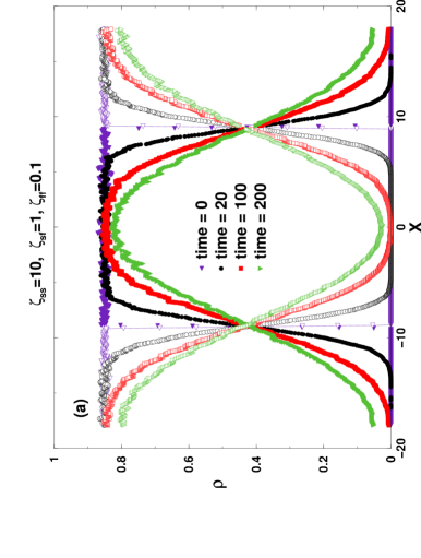
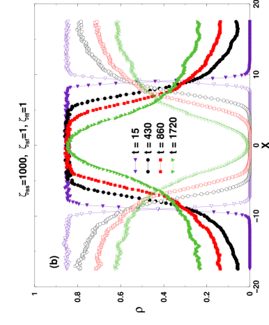
Figure 1:

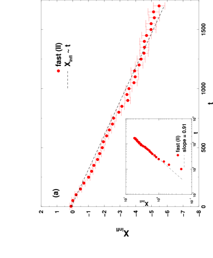
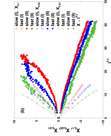
Figure 2:

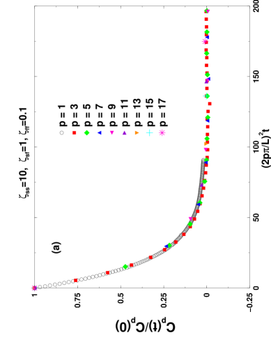
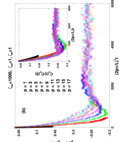
Figure 3:

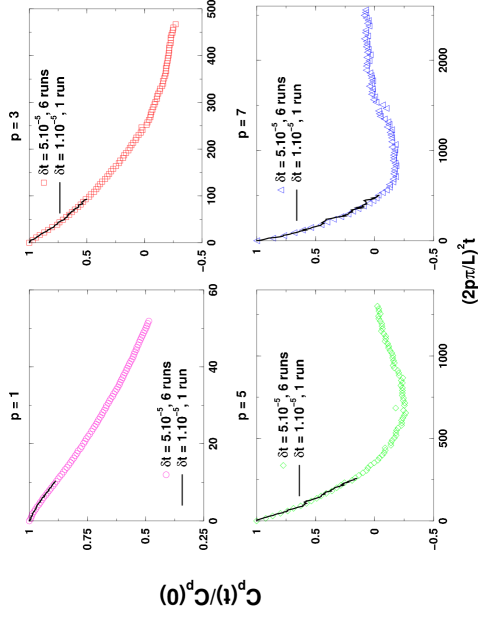
Figure 4:

References

- (1) J. Crank, The Mathematics of Diffusion, Oxford University Press, Oxford, 1956, Ch. 11, p. 254.
- (2) G. S. Hartley, Trans. Faraday Soc. 42B, 6 (1946).
- (3) T. K. Kwei and H. M. Zupko, J. Polym. Sci. A2 7, 867 (1969).
- (4) C. Y. Hui, K. C. Wu, R. C. Lasky, and E. J. Kramer, J. Appl. Phys. 61, 5129(1987); 61, 5137(1987).
- (5) E. Gattiglia and T. P. Russell, J. Polym. Sci. 27, 2131 (1989).
- (6) A. Peterlin, Die Makromolekulare Chemie 124, 136 (1969).
- (7) T. T. Wang, T. K. Kwei, and H. L. Frisch, J. Polym. Sci. A2 7, 2019 (1969).
- (8) T. K. Kwei, T. T. Wang, and H. M. Zupko, Macromolecules 5, 645 (1972).
- (9) A. S. Argon, R. E. Cohen, and A. C. Patel, Polymer 40, 6991 (1999).
- (10) W.-L. Wang, J. R. Chen, and S. Lee, J. Mater. Res. 14, 4111 (1999).
- (11) A. Elafif, M. Grmela, and G. Lebon, J. Non-Newtonian Fluid Mech. 86, 253 (1999).
- (12) T. P. Witelski, J. Polym. Sci. B 34, 141(1996).
- (13) S. Swaminathan and D. A. Edwards, Appl. Math. Lett. 17, 7(2004).
- (14) N. L. Thomas and A. H. Windle, Polymer 19, 255 (1978); 21, 613 (1980); 22, 627 (1981); 23, 529 (1982).
- (15) G. Rossi and K. A. Mazich, Phys. Rev. E 48, 1182 (1993).
- (16) G. Rossi, P. A. Pincus and P. G. de Gennes, Europhys. Lett. 32, 391 (1995).
- (17) A. Friedman and G. Rossi, Macromolecules 30, 153 (1997).
- (18) T. Qian and P. L. Taylor, Polymer 41, 7159 (2000).
- (19) G. Perera, R. H. Doremus, and W. Lanford, J. Am. Ceram. Soc. 74, 1269 (1991).
- (20) M. Tsige and G. S. Grest, J. Chem. Phys. 120, 2989 (2004).
- (21) M. Tsige and G. S. Grest, J. Chem. Phys. 121, 7513 (2004).
- (22) A. Kopf, B. Dünweg, and W. Paul, J. Chem. Phys. 107, 6945 (1997).
- (23) B. Dünweg, J. Chem. Phys. 99, 6977 (1993).
- (24) B. Dünweg, in Computer Simulations of Surfaces and Interfaces, edited by B. Dünweg, D. P. Landau, and A. I. Milchev, Kluwer Academic Publishers, Dordrecht (2003), p. 77.
- (25) P. Espanol and P. Warren, Europhys. Lett. 30, 191 (1995).
- (26) T. Soddemann, B. Dünweg, and K. Kremer, Phys. Rev. E 68, 046702 (2003).