Universal behavior at discontinuous quantum phase transitions

Abstract

Discontinuous quantum phase transitions besides their general interest are clearly relevant to the study of heavy fermions and magnetic transition metal compounds. Recent results show that in many systems belonging to these classes of materials, the magnetic transition changes from second order to first order as they approach the quantum critical point (QCP). We investigate here some mechanisms that may be responsible for this change. Specifically the coupling of the order parameter to soft modes and the competition between different types of order near the QCP. For weak first order quantum phase transitions general results are obtained. In particular we describe the thermodynamic behavior at this transition when it is approached from finite temperatures. This is the discontinuous equivalent of the non-Fermi liquid trajectory close to a conventional QCP in a heavy fermion material.

I Introduction

Recently, the subject of discontinuous quantum phase transitions has received much attention flouquet . Besides the theoretical interest in these transitions there are many new experimental results showing that they occur in heavy fermions and magnetic transition metal compounds first ; Belitz . In these materials as one approaches a quantum critical point, the transitions change their nature from second to first order first . There are many mechanisms which can drive a second order transition into a first order one. For example, in compressible magnets, pressure may produce this change boccara . In antiferromagnets boccara and superconductors paglione this may be accomplished by an external uniform magnetic field . Here we will be interested in more subtle mechanisms which arise due to a coupling of the order parameter to fluctuations russos . In this case the effects are weaker being associated with what is generally known as weak first order transitions. These mechanisms become more relevant at very low temperatures where quantum fluctuations are important.

The fluctuations we consider are of different types. In the first case they are soft modes and as a paradigm of this case we study the coupling of the superconductor order parameter to the electromagnetic field. This has been investigated by Halperin, Lubensky and Ma haluma but, since we are interested in the fully quantum mechanical case at zero temperature, our problem becomes similar to that treated by Coleman and Weinberg in particle physics Coleman . Next, we consider the effect of coupling the order parameter of a given phase to fluctuations of a different phase which competes with the former in the same region of the phase diagram. This problem is particularly relevant for heavy fermion systems where an inhomogeneous state consisting of antiferromagnetic and superconducting regions has been observed kawasaki . This coupling between competing order parameters gives rise to new effects compared with the previous situation. In this case not only the nature of the quantum transitions may change but the ordered phase itself may become an inhomogeneous mixture with different values for the order parameter.

We obtain general features of the behavior of a system approaching a weak first order quantum phase transition (WFOQPT) from finite temperatures. In spite that the correlation length does not diverge as $T\rightarrow 0$, scaling does apply for these WFOQPT and allows for a general description of this phenomenon.

II Coupling to soft modes: The Coleman-Weinberg mechanism

A well known case of quantum fluctuations inducing a weak first order transition is the Coleman -Weinberg mechanism Coleman . In the solid-state version, we consider a superconductor represented by a complex field $(\varphi_{1},\varphi_{2})$ coupled to the electromagnetic field MucioBook ; PhysicaA . The Lagrangian density of the model is given by,

$$L =-\frac{1}{4}(F_{\mu\nu})^{2}\!+\!\frac{1}{2}(\partial_{\mu}\varphi_{1}\!+\!qA_{\mu}\varphi_{2})^{2}+$$

$$+\frac{1}{2}(\partial_{\mu}\varphi_{2}-qA_{\mu}\varphi_{1})^{2}+$$

$$-\frac{1}{2}m^{2}(\varphi_{1}^{2}+\varphi_{2}^{2})-\frac{\lambda}{4!}(\varphi_{1}^{2}+\varphi_{2}^{2})^{2}.$$ (1)

We are using $\hbar=c=1$ units and the indices $\mu,\nu$ run from $0$ to $d=3$. In Eq. (II) space and time are isotropic and consequently the dynamic critical exponent $z=1$. For a neutral superfluid $(q=0)$ the system decouples from the electromagnetic field and has a continuous, zero temperature superfluid-insulator transition at $m^{2}=0$ (see Fig. 1).

The effective potential method Jona ; ColemanBook ; Jackiw yields the quantum corrections to the action given by the Lagrangian density of Eq. (II). At $T=0$ in the one loop approximation, the effective potential close to the transition ($m\approx 0$) is given by MucioBook

$$V_{eff}=\frac{1}{2}m^{2}\varphi^{2}+\frac{\lambda}{4!}\varphi^{4}+\frac{3q^{4}}{64\pi^{2}}\varphi^{4}\left[\ln\left(\frac{\varphi^{2}}{M^{2}}\right)-\frac{25}{6}\right]$$ (2)

where $M$ comes from renormalization and is completely arbitrary Coleman . We can take the value of $M$ as the minimum of the effective potential $\langle\varphi\rangle$. In this case we have the equation, for $M=\langle\varphi\rangle$,

$$m^{2}+\frac{\lambda}{6}\langle\varphi\rangle^{2}-\frac{11q^{4}}{16\pi^{2}}\langle\varphi\rangle^{2}=0$$ (3)

which yields

$$\langle\varphi\rangle^{2}=\frac{m^{2}}{\left(\frac{\lambda}{6}-\frac{11q^{4}}{16\pi^{2}}\right)}$$ (4)

or alternatively for $\lambda$

$$\lambda=-\frac{6m^{2}}{\langle\varphi\rangle^{2}}+\frac{33q^{4}}{8\pi^{2}}.$$ (5)

We can use the equation above to remove $\lambda$ from the effective potential Eq. (2) introducing another free parameter, namely the non-trivial minimum of the effective potential $\langle\varphi\rangle$. In this case, Eq. (2) reads

$$V_{eff}\!=\!\frac{1}{2}m^{2}\varphi^{2}\!-\!\frac{m^{2}}{4\langle\varphi\rangle^{2}}\varphi^{4}\!+\!\frac{3q^{4}}{64\pi^{2}}\varphi^{4}\left[\ln\left(\frac{\varphi^{2}}{\langle\varphi\rangle^{2}}\right)\!-\!\frac{1}{2}\right].$$ (6)

The change of the parameters above known as dimensional transmutation Coleman can only be done if the effective potential has a non-trivial minimum $\langle\varphi\rangle\neq 0$ as is clear from the equations above. Since close to the transition $m\approx 0$, we conclude from Eqs. (3) and (4) that the condition for such a minimum to exist is

$$\lambda\sim q^{4}.$$ (7)

Now let’s define the coherence length

$$\xi=\sqrt{1/2|m^{2}|}$$ (8)

and the London penetration depth

$$\lambda_{L}=\sqrt{1/2q^{2}|\langle\varphi\rangle|^{2}}$$ (9)

as is usually done for Ginzburg-Landau models. We can show that the condition of Eq. (7) is equivalent to

$$\lambda_{L}\ll\xi.$$ (10)

This is the same condition for the occurrence of weak first order transitions obtained in Ref. haluma . However, in general, if $\lambda_{L}\sim\xi$, fluctuations of the order parameter can destabilize the Coleman-Weinberg mechanism and the resulting quantum transitions can be second order (see Ref. Belitz ).

The condition (10) can be obtained from our results as follows. The ratio $\lambda_{L}/\xi$, from Eq. (8) and Eq. (9), is

$$\frac{\lambda_{L}}{\xi}=\sqrt{\frac{|m^{2}|}{q^{2}|\langle\varphi\rangle^{2}|}}.$$ (11)

Substituting the result of Eq. (4) we get

$$\frac{\lambda_{L}}{\xi}=\sqrt{\frac{1}{q^{2}}\left|\frac{\lambda}{6}-\frac{11q^{4}}{16\pi^{2}}\right|}.$$ (12)

This ratio is independent of $m^{2}$ as expected and it is clear that, if $\lambda\sim q^{4}$, we have $(\lambda_{L}/\xi)\ll 1$ or $\lambda_{L}\ll\xi$ as expected. We will discuss more about this condition later in section V.

Let us consider that $\lambda\sim q^{4}$ (or equivalently $\lambda_{L}\ll\xi$) and study the minima of the effective potential, Eq. (6). We find that at a critical value of the mass, given by

$$m_{c}^{2}=\frac{3q^{4}}{32\pi^{2}}\langle\varphi\rangle^{2}$$ (13)

there is a first order transition to a superconducting state. Notice that the transition in the neutral superfluid ($q=0$) is continuous rather than first order and takes place at $m^{2}=0$. Therefore, quantum fluctuations due to the coupling to soft modes, the photons, lead to symmetry breaking in the normal region of the phase diagram of the neutral superfluid. This occurs close to the quantum critical point of the chargeless system extending the region where a symmetry broken phase appears in the phase diagram. The transition occurs at a finite value of the mass $m_{c}^{2}$ and is first order. The shift of the critical mass depends on a power of the coupling of the order parameter to the soft modes, in the present case the charge of the Cooper pairs.

Introducing a parameter $g=m^{2}-m_{c}^{2}$ which measures the distance to the transition, we can write the effective potential at $T=0$ as,

$$V_{eff}=\frac{1}{4}\langle\varphi\rangle^{2}|m^{2}-m_{c}^{2}|\propto|g|^{2-\alpha}$$ (14)

with the exponent value $\alpha=1$ reflecting the fact the transition is first order PhysicaA . The associated latent heat is $L_{h}=\frac{1}{4}m_{c}^{2}\langle\varphi\rangle^{2}$. Spinodals points at $T=0$ can also be calculated PhysicaA .

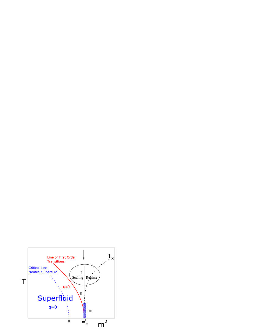
Figure 1: Phase diagram of a charged superfluid coupled to photons. For completeness we show also the critical line of the neutral superfluid. Along the trajectory $m^{2}=m_{c}^{2}$ one can distinguish different regimes as explained in the text.

The finite temperature case can be studied replacing the frequency integrations in the calculation of the effective potential by sums over Matsubara frequencies MucioBook . The generalization of the effective potential to finite temperatures close to the transition can be written as PhysicaA

$$V_{eff}(T) =\frac{1}{4}m^{2}\langle\varphi\rangle^{2}|g|\!\left[1+\right.$$

$$\left.+\frac{2}{\pi^{2}m^{2}\langle\varphi\rangle^{2}}\frac{T^{d+1}}{|g|}I_{d}\!\left(\frac{M(\varphi)}{T}\right)\!\right]$$ (15)

where the integral $I$ is given by

$$I_{d}(y)=\int_{0}^{\infty}dxx^{d-1}\ln{\left[1-e^{-\sqrt{x^{2}+y^{2}}}\right]}.$$ (16)

and $M(\varphi)=m^{2}+q^{2}\varphi^{2}$. The function $I_{3}(y)=I(y)$ can be obtained numerically integrating Eq. (16).

The finite temperature phase diagram is shown in Fig. 1. For completeness we show the critical line of the neutral superfluid, $T_{SF}=|m^{2}|^{\psi}$, which is governed by the shift exponent ${\psi}^{-1}=z/(d+z-2)=1/2$ in $d=3$ (see Ref. MucioBook ). The new line of first order transitions is given by $T_{c}=\sqrt{m_{c}^{2}-|m^{2}|}$.

III Scaling at a weak first order quantum transition

We will now consider the system sitting at the new quantum phase transition point, i.e., at $m^{2}=m_{c}^{2}$ and decrease the temperature. This is the equivalent of the non-Fermi liquid trajectory for ordinary quantum critical points in metallic systems.

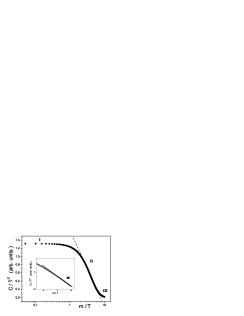
Figure 2: The temperature dependent specific heat along the trajectory $m^{2}=m_{c}^{2}$ of the zero temperature first order transition. The different regimes are discussed in the text. Notice the dashed straight line that indicates the $\ln T$ behavior in regime II.

For high temperatures, $T\gg m_{c}$, which corresponds to the regime I of Fig. 1 and Fig. 2, the function $I_{3}(y)$ saturates, $I_{3}(y<0.12)\approx-2.16$. In this case the effective potential,

$$V_{eff}(T)\approx\frac{1}{4}m^{2}\langle\varphi\rangle^{2}|g|\bigg{\{}1-\frac{4.32}{\pi^{2}m^{2}\langle\varphi\rangle^{2}}\frac{T^{d+1}}{|g|}\bigg{\}}$$

and can be cast in the scaling form,

$$V_{eff}(T)\propto|g|^{2-\alpha}F\left[\frac{T}{T_{\times}}\right].$$

with $F(0)=$ $constant$. This scaling form is reminiscent of that for the free energy close to a quantum critical point. In the present case of a discontinuous zero temperature transition, the critical exponent PhysicaA $\alpha=1$ and the characteristic temperature is,

$$T_{\times}\propto|g|^{\nu z}\propto|g|^{\frac{z}{d+z}}=|g|^{\frac{1}{d+1}}=|g|^{\frac{1}{4}}$$

with $\nu=1/(d+z)$ PhysicaA . In this regime I or scaling regime, along the line $m^{2}=m_{c}^{2}$ shown in Fig. 1, the free energy density has therefore the scaling form $f(m=m_{c},T)\propto T^{(d+z)/z}$ and the specific heat as shown in Fig. 2 is given by,

$$C/T\big{|}_{(m=m_{c},T)}\propto T^{\frac{d-z}{z}}.$$ (17)

Then the thermodynamic behavior along the line $m^{2}=m_{c}^{2}$ in regime I ($T\gg m_{c}$) is the same as when approaching the quantum critical point of the neutral superfluid, along the critical trajectory $m^{2}=0$. The system is unaware of the change in the nature of the zero temperature transition and at such high temperatures charge is irrelevant.

When further decreasing temperature along the line $m^{2}=m_{c}^{2}$ there is an intermediate, non-universal regime (regime II in Figs. 1 and 2). In the present case for $m_{c}<T$ the specific heat $C/T^{d/z}\propto\ln T$ as can be seen from the dashed straight line shown in the semi-log plot of Fig. 2.

Finally, at very low temperatures, for $T<<m_{c}$ and $m^{2}=m_{c}^{2}$, i.e., in regime III of Fig. 2, the specific heat vanishes exponentially with temperature, $C/T^{d/z}\propto\exp(-m_{c}/T)$. The gap for thermal excitations is given by the shift $m_{c}$ of the quantum phase transition. The correlation length which grows along the line $m^{2}=m_{c}^{2}$ with decreasing temperature reaches saturation in regime III at a value $\xi_{S}\approx m_{c}^{-1}$. Then, we can understand the exponential dependence of the specific heat as due to gapped excitations inside superconducting bubbles of finite size $L\thicksim\xi$. The gap between the states in the bubbles is $\Delta\sim L^{-z}\sim\xi^{-z}\sim m_{c}$ as we have found previously.

Although the results above have been obtained for a particular model, the behavior in the scaling regime I and III should be universal and characteristic of any weak first order quantum transition. Notice that the relevant critical exponents which determine the scaling behavior in particular in regime I are those associated with the QCP of the uncoupled system which in the present case is the neutral superfluid.

IV Coupling between order parameters

IV.1 Quantum first order transitions in superconducting heavy-fermions

Weak first order transitions and spontaneous symmetry breaking near quantum phase transitions can also occur due to the coupling of an order parameter to nearly critical fluctuations of another phase. This provides a new mechanism for WFOQPT besides the coupling to gapless excitations as treated above and in Ref. Belitz for example (see also Refs. note ; berker ).

In this section we study the coupling, at $T=0$, of an order parameter to fluctuations of a competing order. This type of coupling becomes important when two different phases are in competition on the same region of the phase diagram. In this case for some values of the microscopic interactions which are close, there are alternative ground states which interfere with one another. This is the situation, for example, of several heavy-fermions Pagliuso and of high-T_c superconductors Kastner where in general the dispute is among superconductivity and antiferromagnetism. We obtain the effects on a given phase, of the coupling of its order parameter to fluctuations of the competing order, in the form of quantum corrections. We show that these can produce spontaneous symmetry breaking and change the nature of the transition even if these fluctuations are non critical. Again, due to the weak first order character of the new phase transition we expect to find scaling behavior as described previously.

We consider the case of a heavy-fermion (HF) system with a superconducting phase that is close to an antiferromagnetic instability at $T=0$ PRB as in Fig. 3. As before, we first describe the superconducting phase by the simplified Lorentz invariant free action as in Eq. (II) but now coupled to an AF order parameter instead of the electromagnetic field. In many cases however the effects of dissipation should be taken into account. Then, later on we use another free action for the superconducting field. This different quadratic form is associated with a dynamic exponent $z=2$, instead of $z=1$ of the Lorentz invariant case Ramazashvili ; Kirkpatrick .

Our model is of the Ginzburg-Landau type and contains three real fields. Two fields, $\phi_{1}$ and $\phi_{2}$, correspond to the two components of the superconductor order parameter. The other field $\phi_{3}$, for simplicity represents a one component antiferromagnetic order parameter. The results are immediately generalized to a three component AF vector field, with the unique consequence of changing some numerical factors PRB . The free functional associated with the magnetic part represented by the field $\phi_{3}$, the sub-lattice magnetization, takes into account the dissipative nature of the paramagnons near the magnetic phase transition Hertz in the metal and yields the propagator

$$D_{0}(\omega,\boldsymbol{q})=\frac{i}{i|\omega|\tau-q^{2}-m_{p}^{2}}$$ (18)

where $\tau$ is a characteristic relaxation time and $m_{p}^{2}$ is related to a local Coulomb repulsion $U$ and the density of states at the Fermi level $N(E_{F})$ by

$$m_{p}^{2}=1-UN(E_{F}).$$ (19)

The part of the action associated with the potential is given by

$$V_{cl}(\phi_{1},\phi_{2},\phi_{3})=\frac{1}{2}m^{2}(\phi_{1}^{2}+\phi_{2}^{2})+\frac{1}{2}m_{p}^{2}\phi_{3}^{2}+$$

$$+V_{s}(\phi_{1},\phi_{2})+V_{p}(\phi_{3})+V_{i}(\phi_{1},\phi_{2},\phi_{3}),$$ (20)

where the self-interaction of the superconductor field is

$$V_{s}(\phi_{1},\phi_{2})=\frac{\lambda}{4!}(\phi_{1}^{2}+\phi_{2}^{2})^{2},$$ (21)

and that of the antiferromagnet is given by

$$V_{p}(\phi_{3})=\frac{g}{4!}\phi_{3}^{4}.$$ (22)

Finally, the last term is the (minimum) interaction between the relevant fields,

$$V_{i}(\phi_{1},\phi_{2},\phi_{3})=u(\phi_{1}^{2}+\phi_{2}^{2})\phi_{3}^{2}.$$ (23)

This term is the first allowed by symmetry on a series expansion of the interaction. Notice that for $u>0$, which is the case here, superconductivity and antiferromagnetism are in competition and this term does not break any symmetry of the original model. However, including quantum fluctuations we show that spontaneous symmetry breaking can occur in the normal phase separating the SC and AF phases. This case is represented schematically in Fig. 3 and is discussed in the subsequent sections.

Figure 3: Normal phase separating SC and AF phases.

IV.2 Superconducting transition

We first consider the metal-superconductor transition in HF when the superconducting field is coupled, as in Eq. (23), to AF fluctuations described by the propagator of Eq. (18)(Fig. 3). Detailed calculation of the effective potential have already been presented PRB . The general result is given by,

$$V_{ef}(\phi_{c})\approx\frac{1}{2}M^{2}\phi_{1c}^{2}+am_{p}^{2}\phi_{1c}^{2}|\phi_{1c}|+\frac{\tilde{\lambda}}{4!}\phi_{1c}^{4}+\mathcal{O}(\phi^{5}).$$ (24)

In Eq. (24), $\tilde{\lambda}$ is a renormalized coupling but of the same order of the bare coupling $\lambda$. The new coupling $a$ introduced by fluctuations can produce a symmetry breaking in the normal state extending the SC region in the phase diagram at $T=0$. The same mechanism turns the transition to weak first order with a small latent heatS.Stat.Comm. . Using the same argument as in the preceding section we can introduce again parameters associated with $\xi$ (coherence length) and $\lambda_{L}$ (London penetration depth) in this case given by

$$\xi=\sqrt{1/2|m^{2}|}$$ (25)

$$\lambda_{L}=\sqrt{1/u|\langle\phi\rangle^{2}|}.$$ (26)

It’s difficult to carry out the dimensional transmutation analytically on the result of Eq. (24) since the equations of minima are hard to solve. However, we can check numerically that the condition for the existence of minima away from the origin is equivalent to $\lambda_{L}\ll\xi$ as in the previous case. It’s also interesting to notice that the first order transition is produced by the cubic term in Eq. (24) and this term is proportional to the magnetic mass $m_{p}$. If magnetic fluctuations were critical, i.e., $m_{p}=0$, the only effect of the coupling would appear as a term proportional to $\phi^{5}$. This term is usually neglected since its power is higher than those initially considered in the classical potential and usually insufficient to create new minima around the origin. Therefore, if AF fluctuations were critical the effects of the quantum corrections in the transition could be neglected.

IV.3 Antiferromagnetic transition

In order to study the magnetic transition, as mentioned previously we consider two kinds of quadratic forms associated with the free superconducting fields. The first is the usual Lorentz invariant free action that we have discussed before in Sec. IV.1. Next we work with another free action which takes into account dissipation and is associated with a $z=2$ dynamics.

Let’s first study the result for the Lorentz invariant propagator. Close to the AF transition we have PRB

$$V_{ef}(\phi_{3c}) \approx\frac{1}{2}M_{p}^{2}\phi_{3c}^{2}++\frac{\tilde{g}}{4!}\phi_{3c}^{4}+\tilde{u}^{2}\phi_{3c}^{4}\ln\left(\frac{\phi_{3c}^{2}}{\langle\phi_{3}\rangle^{2}}\right)$$

$$+\tilde{u}m^{2}\phi_{3c}^{2}\ln{\left(\frac{\phi_{3c}^{2}}{\langle\phi_{3}\rangle^{2}}\right)}$$ (27)

We notice directly from Eq. (IV.3) that if the superconductor order parameter fluctuations were critical we would obtain the same result of Eq. (6) since in this case the parameter $m^{2}=0$. However, SC fluctuations are not critical but close to criticality and the last term of Eq. (IV.3) may become important. Of course, its relevance depends on the strength of the renormalized coupling $\tilde{u}$ and the results considering this term leads to new and interesting changes in the ground state. We obtain, besides the two finite minima of the Coleman-Weinberg potential of Eq. (6), two extra minima very close to the origin PRB . The normal state associated with these minima has a small moment since the value of the order parameter is related to the sub-lattice magnetization. An additional first order transition occurs when the other two minima away from the origin become the stable ones as the system moves away from the superconductor instability. This transition is from a small moment AF (SMAF) to a large moment AF (LMAF) and occurs even before the continuous mean field transition. When we move away from the magnetic transition the strength of this new term decreases with the value of $m^{2}$ and the two new minima move to the origin producing a normal state with vanishing magnetization again. It’s important to note here that the SMAF is obtained because the magnetic order parameter couples to fluctuations which are close to criticality but not critical. Critical fluctuations yield the same results of section II.

Now, for many cases of interest, SC fluctuations are better described by a dissipative propagator associated with a $z=2$ dynamicsRamazashvili ; Kirkpatrick similar to Eq. (18). This is useful to account for pair breaking interactions as magnetic impurities that can destroy superconductivity Sigrist ; Mineev . It is given by,

$$G_{0}(\omega,\boldsymbol{q})=\frac{i}{i|\omega|\tau^{\prime}-q^{2}-m^{2}}.$$ (28)

The parameter $m^{2}$ is still related with the classical distance from the phase transition and we have a relaxation time $\tau^{\prime}$. In general we also have a non-dissipative term (as in the case studied above) but this term is neglected since the linear term is the most important in the low frequency region. Calculation of the effective potential is very similar to the previous cases and the result has the form

$$V_{eff}=\frac{1}{2}M_{p}^{2}\phi_{3}^{2}+\frac{1}{4!}\tilde{g}\phi_{3}^{4}+\frac{1}{15\pi^{2}}(2u\phi_{3}^{2}+m^{2})^{5/2}$$ (29)

where the renormalized mass is

$$M_{p}=m_{p}^{2}-\frac{2}{3\pi^{2}}m^{3}u-\frac{1}{12\pi^{2}}m_{p}^{3}g$$ (30)

and the renormalized coupling

$$\tilde{g}=g-\frac{12}{\pi^{2}}mu^{2}-\frac{3}{8\pi^{2}}m_{p}g^{2}.$$ (31)

Quantum corrections can once again produce a weak first order transition. We note that in this case the renormalization of the potential obtained is easier since there are no logarithmic terms to renormalize PRB . Anyway, the result is very similar to that presented in section IV.2 since we have equivalent propagators for the fluctuations. In general the form of the quantum correction depends not only on the effective dimension of the uncoupled QCP but also on the form and specially the dynamics of the soft modes or competing fluctuations.

The transformation $(\phi_{3}^{\prime})^{2}=2u\phi_{3}^{2}+m^{2}$ makes the potential of Eq. (29) simpler and the analysis of its extrema shows that the transition can be first order depending on the coupling values. The appearance of SMAF phases is not possible in this case. We note, however, that the couplings are dependent on the renormalization parameter $M$ defined in Sec. II and a renormalization group approach is essential to make the results more reliable. In the next section we illustrate this with an analysis of the Coleman-Weinberg case.

V One-loop effective potentials and renormalization group

In the previous sections we have obtained weak quantum first order transitions from minima generated balancing terms in the effective potential. This is possible when we compare terms of the same order and therefore the minima depend on the values of the couplings. Considering, for example, the superconductor coupled to the electromagnetic field, the terms we have to balance are proportional to $\lambda$ and $q^{4}$. New minima away from the origin are produced if

$$\lambda\sim q^{4}$$ (32)

and this condition also leads to a relation for the London penetration depth and the coherence length $\lambda_{L}\ll\xi$. In this section we show how we can use renormalization group arguments to generalize the results for any small $\lambda$ and $q$ and get rid of the condition (32).

When deriving Eq. (2) we have introduced a new parameter $M$, associated with a renormalization mass and which was completely arbitrary. The results for the model must be the same for any chosen value of $M$. Now, if we prove that a variation in the value of $M$ produces a correspondent variation in the coupling constant $\lambda$, it’s always possible to satisfy the condition (32) choosing a suitable value of $M$. To prove that, we have to consider Eq. (2). We want to rewrite this equation with a value $M^{\prime}$, such that,

$$V_{eff} =\frac{1}{2}m^{2}\varphi^{2}+\frac{\lambda}{4!}\varphi^{4}+\frac{3q^{4}}{64\pi^{2}}\varphi^{4}\left[\ln\left(\frac{\varphi^{2}}{{M^{\prime}}^{2}}\frac{{M^{\prime}}^{2}}{M^{2}}\right)-\frac{25}{6}\right]$$

$$V_{eff} =\frac{1}{2}m^{2}\varphi^{2}+\frac{\lambda}{4!}\varphi^{4}+\frac{3q^{4}}{64\pi^{2}}\varphi^{4}\ln\frac{{M^{\prime}}^{2}}{M^{2}}+$$

$$\frac{3q^{4}}{64\pi^{2}}\varphi^{4}\left[\ln\left(\frac{\varphi^{2}}{{M^{\prime}}^{2}}\right)-\frac{25}{6}\right]$$

which is equivalent to Eq. (2) with the reparametrization

$$\frac{\lambda^{\prime}}{4!}=\frac{\lambda}{4!}+\frac{3q^{4}}{64\pi^{2}}\ln\frac{{M^{\prime}}^{2}}{M^{2}}.$$ (33)

In this sense the effective potential is always given by the same equation with a suitable parametrization of the coupling.

This argument can be formally stated in an renormalization group approach and we refer to the correspondent section of Ref. Coleman . As a result, a weak first order transition occurs for any small values of $\lambda$ and $q$, since we can appropriately choose the renormalization mass. The only restriction comes from perturbation theory which requires small couplings.

For the case of coupling between AF and SC order parameters we can also construct a renormalization group. Within this approach we expect to find all the conditions for the occurrence of weak first order transitions. Detailed calculations and results will be published elsewhere.

VI Conclusions

We have studied the effects on a phase transition of coupling the order parameter of this phase to soft modes or to fluctuations of a competing phase. Since these effects become more important at low temperatures we have mostly considered the zero temperature case. We have obtained the effects of quantum corrections due to this coupling on the quantum critical point associated with the relevant order parameter. These corrections were calculated using the effective potential method. They can produce radical modifications on the nature of the original phase transition. They can change the nature of the transition, from continuous to discontinuous and also affect the ordered phase itself giving rise to an inhomogeneous phase with two values of the order parameter.

Whenever the fluctuations change the nature of the transition to weak first order, we can study them using a scaling approach. We have obtained explicit results for one particular case but that should hold in general. As the system approaches the discontinuous transition from non-zero temperature, we can distinguish three different regimes. In the first, the high temperature regime, the scaling behavior is the same as approaching the quantum critical point of the uncoupled system, i.e., in the absence of additional fluctuations or soft modes. Further decreasing the temperature there is a non-universal regime which may depend on the particular dynamics of the original system and of the nature of the additional modes. Finally at the lowest temperatures there is a regime which is characteristic of the first order nature of the zero temperature transition. At such low temperatures the correlation length saturates at a finite value. The thermodynamic properties have a contribution which is thermally activated. This can be traced to excitations which are gapped due to finite size effects as they occur in finite bubbles of the incipient phase. The correctness of this interpretation is clear from the fact that the gap for excitations is inversely related to the size of the bubbles which in turn is of the order of the correlation length. Notice also that the former is related to the shift in the zero temperature phase transition with respect to that of the uncoupled system.

The relevant exponents which determine the scaling behavior near the weak first order transition are those associated with the quantum critical point of the uncoupled system, i.e., of the system in the absence of competing fluctuations or soft modes. In particular this is the case of the dynamic exponent. The scaling properties of the new transition are related to the existence of an underlying second order instability which has become discontinuous due to the effects of soft modes or of fluctuations of a competing order parameter.

- (1) J. Flouquet, cond-mat/0501602 and to be published.
- (2) S. Kawasaki, et al.,Phys. Rev. Lett. 91, 137001 (2003); Y. Kitaoka, S. Kawasaki, T. Mito, Y. Kawasaki, to appear in J. Phys. Soc. JPN, 74, No.1 (2005); W. Yu, et al. Phys. Rev. Lett. 92, 086403 (2004). M. Uhlarz, C. Pfleiderer, and S. M. Hayden Phys. Rev. Lett. 93, 256404 (2004);C. Pfleiderer and A. D. Huxley Phys. Rev. Lett. 89, 147005 (2002);A. Bianchi, R. Movshovich, N. Oeschler, P. Gegenwart, F. Steglich, J. D. Thompson, P. G. Pagliuso, and J. L. Sarrao Phys. Rev. Lett. 89, 137002 (2002);C. Pfleiderer et al., Nature (London) 412, 58 (2001);N. Kimura, M. Endo, T. Isshiki, S. Minagawa, A. Ochiai, H. Aoki, T. Terashima, S. Uji, T. Matsumoto, and G. G. Lonzarich Phys. Rev. Lett. 92, 197002 (2004)
- (3) D. Belitz, T.R. Kirkpatrick and T. Vojta, cond-mat/0403182, to appear in Rev. Mod. Phys..
- (4) see N. Boccara, Symétries Brisées, Hermann, Paris, (1979), p.120.
- (5) J. Paglione, M. A. Tanatar, D. G. Hawthorn, E. Boaknin, R. W. Hill, F. Ronning, M. Sutherland, L. Taillefer, C. Petrovic, and P. C. Canfield Phys. Rev. Lett. 91, 246405 (2003).
- (6) S. A. Brazovskii, Sov. Phys. JETP 41, 85 (1975); S. A. Brazovskii and S.G. Dmitriev, Sov. Phys. JETP 42, 497 (1976); A.M. Dyugaev, Sov. Phys. JETP 56, 567 (1983).
- (7) B. I. Halperin, T. Lubensky and S.K. Ma, Phys. Rev. Lett. 32, 292 (1974).
- (8) S. Coleman and E. Weinberg, Phys. Rev. D 7, 1888 (1973).
- (9) see Y. Kitaoka, et al in Ref. first .
- (10) See M. A. Continentino, Quantum Scaling in Many-Body Systems, World Scientific, Singapore, (2001), chapter 12.
- (11) M. A. Continentino and A. S. Ferreira, Physica A 339, 461-468 (2004).
- (12) G. Jona-Lasinio, Nuovo Cimento 34, 1790 (1964).
- (13) S. Coleman, Aspects of Symmetry, Cambridge University Press (1985) chapter 5.
- (14) R. Jackiw, Phys. Rev. D 9 1686 (1973).
- (15) The concept of generic scale invariance (GSI) has been emphasized recently with respect to systems with continuous broken symmetry Belitz . In the simplest case of a Heisenberg ferromagnet in an external magnetic field () GSI is related to the strong coupling fixed point at , which governs the symmetry broken phase. Close to this attractor, and . The free energy density scales as, . Then , the magnetization and the susceptibility . An additional contribution arises at , , namely . This yields and for berker .
- (16) M. E. Fisher and A. N. Berker, Phys. Rev. B 026, 2507 (1982).
- (17) V.A. Sidorov , M. Nicklas, P.G. Pagliuso, J.L. Sarrao, Y. Bang, A.V. Balatsky, J.D. Thompson Phys. Rev. Lett. 89, 157004 (2002); P. G. Pagliuso, N. O. Moreno, N. J. Curro, J. D. Thompson, M. F. Hundley, J. L. Sarrao, Z. Fisk, A. D. Christianson, A. H. Lacerda, B. E. Light and A. L. Cornelius., Phys. Rev. B66, 054433 (2002); M. Nicklas, V. A. Sidorov, H. A. Borges, P. G. Pagliuso, C. Petrovic, Z. Fisk, J. L. Sarrao, and J. D. Thompson, Phys.Rev. B67, 020506 (2003); R. A. Fisher, F. Bouquet, N. E. Phillips, M. F. Hundley, P. G. Pagliuso, J. L. Sarrao, Z. Fisk, and J. D. Thompson, Phys.Rev. B65, 224509 (2002).
- (18) Kastner MA, Birgeneau RJ, Shirane G, Endoh Y, Rev. Mod. Phys. 70 (3): 897-928 (1998); S. C. Zhang, Science 275, 1089 (1997).
- (19) A. S. Ferreira, M. A. Continentino and E. C. Marino, Phys. Rev. B 70, 174507 (2004).
- (20) R. Ramazashvili and P. Coleman, Phys. Rev. Lett. 79, 3752 (1997)
- (21) T. R. Kirkpatrick and D. Belitz, Phys. Rev. Lett. 79, 3042 (1997).
- (22) J. A. Hertz, Phys. Rev. B 14, 1165 (1976).
- (23) At we associate the expression latent heat to a latent work. In this case the latent work is small since it is proportional to in which is the value of the critical mass where the transition occurs. See A. S. Ferreira, M. A. Continentino and E. C. Marino, Sol. St. Comm. 130, 321 (2004).
- (24) V. P. Mineev and M. Sigrist, Phys. Rev. B 63, 172504 (2001).
- (25) V. P. Mineev, JETP Lett. 66, 693 (1997).