Some properties of evolution equation for homogeneous nucleation period under the smooth behavior of initial conditions

Abstract

The properties of the evolution equation have been analyzed. The uniqueness and the existence of solution for the evolution equation with special value of parameter characterizing intensity of change of external conditions, of the corresponding iterated equation have been established. On the base of these facts taking into account some properties of behavior of solution the uniqueness of the equation appeared in the theory of homogeneous nucleation has been established. The equivalence of auxiliary problem and the real problem is shown.

1 Formulation of the problem

In [1] the evolution equation for the nucleation period has been derived. Here we shall analyze the properties of the evolution equation and the uniqueness and existence of the solution of special problems appeared in the theory of nucleation.

Consider the initial problem formulated in [1]

• The following equation is given

  $$g(z)=f_{*}\int_{-\infty}^{z}(z-x)^{3}\exp(cx-\Gamma g(x)/\Phi_{*})dx$$ (1)

  with positive parameters $f_{*}$, $\Gamma$, $\Phi_{*}$, $c$, which are chosen to satisfy condition

  $$\frac{dg(z)}{dz}|_{z=0}=c\Phi_{*}/\Gamma$$ (2)

Equation (1) and condition (2) form the initial problem.

This problem as well as all other ones is considered in a class of continuous functions.

Instead of the function $g$ we introduce the function $G=\Gamma g/\Phi_{*}$. Then we get

$$G(z)=(f_{*}\Gamma/\Phi_{*})\int_{-\infty}^{z}(z-x)^{3}\exp(cx-G(x))dx$$

$$\frac{dG(z)}{dz}|_{z=0}=c$$

We change the variables

$$z\rightarrow(f_{*}\Gamma/\Phi_{*})^{-1/4}z^{\prime}$$

$$x\rightarrow(f_{*}\Gamma/\Phi_{*})^{-1/4}x^{\prime}$$

The new variables will be marked by the same letters $z,x$.

Then we get

$$G(z)=\int_{-\infty}^{z}(z-x)^{3}\exp(c(f_{*}\Gamma/\Phi_{*})^{-1/4}x-G(x))dx$$

$$\frac{dG(z)}{dz}|_{z=0}=c(f_{*}\Gamma/\Phi_{*})^{-1/4}$$

We denote $c(f_{*}\Gamma/\Phi_{*})^{-1/4}$ also as $c$. The value $G$ will be denoted as $g$. We come to the following problem

• The following equation

  $$g(z)=\int_{-\infty}^{z}(z-x)^{3}\exp(cx-g(x))dx$$ (3)

  is given with the positive parameter $c$, chosen to satisfy

  $$\frac{dg(z)}{dz}|_{z=0}=c$$ (4)

The equation (3) and the condition (4) form the reduced problem.

So, here only one parameter $c$ remains.

It is more convenient to consider instead of $g$ the function

$$\phi=cx-g$$

Then we come to the following problem (Problem A)

• The following equation

  $$cz=\phi(z)+\int_{-\infty}^{z}(z-x)^{3}\exp(\phi(x))dx$$ (5)

  is given with the positive parameter $c$, chosen to satisfy

  $$\frac{d\phi(z)}{dz}|_{z=0}=0$$ (6)

Equation (5) and the condition (6) form the problem A. This problem will be the auxiliary problem.

Consider now the problem B

• The following equation

  $$3\int_{-\infty}^{0}y^{2}\exp(\phi(y))dyz=\phi(z)+\int_{-\infty}^{z}(z-x)^{3}\exp(\phi(x))dx$$ (7)

  is given

Only the equation (7) forms the problem B.

We see that the problem B has no parameters.

The main goal of investigation will be to see the uniqueness of the solution of the problem B.

2 Solution of equation (5) with fixed $c$

2.1 Some properties of solution

At first we consider (5) with some positive $c$.

We rewrite (5) for function $g$ in the form

$$g(z)=\int_{-\infty}^{z}(z-x)^{3}\exp(cx-g(x))dx$$

One can see the following property

If the solution exists, then

$$g(z)>0$$

for any $z$

This property goes from the positivity of sub-integral function.

We introduce the iterated equation

$$g(z)=\int_{-\infty}^{z}(z-x)^{3}\exp(cx-\int_{-\infty}^{x}(x-y)^{3}\exp(cy-g(y))dy)dx$$ (8)

We also introduce the nonlinear operator $P$ according to

$$P(s)=\int_{-\infty}^{z}(z-x)^{2}\exp(cx-s(x))dx$$

One can prove the following fact:

If for any $x$ the following inequality

$$g_{1}(x)>g_{2}(x)$$

takes place, then

$$P(g_{1}(x))<P(g_{2}(x))$$

takes place for any $x$.

It follows from the explicit form of $P$.

One can also see the following fact

If the solution exists then

$$g(z)<\exp(cz)/6$$

for any $z$

It follows from the positivity of exponent in the sub-integral function.

We construct iterations according to

$$g_{i+1}=P(g_{i})$$

As the initial approximation we choose

$$g_{0}=0$$

We see that

$$g_{2}>0$$

for any value of the argument

It follows from the positivity of exponent and the whole sub-integral function.

Form the statements formulated above it follows the following chain of inequalities

$$0=g_{0}<g_{2}<g_{4}<....<g<....<g_{5}<g_{3}<g_{1}$$

for any value of the argument.

So, the odd iterations converge and the even iterations converge. So, the solution of the iterated equation exists. But the uniqueness isn’t yet proven.

For any initial approximation which is always positive the iterations with initial $g_{0}=0$ estimate them from above.

Since the r.h.s. is positive and solution has to be positive, the iterations with any initial approximation have to be positive starting from some number (the asymptotics at small arguments are written explicitly). Correspondingly, later the iterations will be estimated by the already constructed iterations. So, the convergence can be estimated to convergence of constructed iterations.

Remark: The analogous iterations have been constructed by F.M.Kuni in 1984, but for the problem B. For the problem B the monotonic functions are absent and it is impossible to prove in such a simple way the convergence of iterations

$$3\int_{-\infty}^{0}y^{2}\exp(\phi_{i}(y))dyz=\phi_{i+1}(z)+\int_{-\infty}^{z}(z-x)^{3}\exp(\phi_{i}(x))dx$$

with

$$\phi_{0}=cx$$

2.2 Uniqueness of solution for small arguments

Now we shall prove the existence and uniqueness of non-iterated equation(5) (in the class of continuous functions)

It can be done by several ways. One of the methods is to introduce the cut-off from the side of small $z$, i.e. to consider only $z>-a$ with big and positive parameter $a$. It was done in [1]. Here we shall use more rigorous method.

We shall show that for given $c$ at

$$z<z_{fin}=\frac{1}{c}\ln[\frac{c^{4}}{6}(1-\epsilon)]$$

with some small positive fixed $\epsilon$ the solution of (5) exists and it is unique.

We construct iterations $g_{i+1}=P(g_{i})$. The starting approximation is not important. We note that they do not go out of the class of positive continuous functions. Under the arbitrary initial approximation, all iterations starting from the first one will be positive.

We have for approximations

$$g_{i+1}-g_{i}=\int_{-\infty}^{z}(x-z)^{3}\exp(cx)(\exp(-g_{i})-\exp(-g_{i-1}))dx$$

Then

$$|g_{i+1}-g_{i}|\leq\int_{-\infty}^{z}(x-z)^{3}\exp(cx)|\exp(-g_{i})-\exp(-g_{i-1})|dx$$

It allows to write the inequality for norms $||...||$ in the functional space $C[-\infty,\infty]$

$$||g_{i+1}-g_{i}||\leq\int_{-\infty}^{z}(x-z)^{3}\exp(cx)||\exp(-g_{i})-\exp(-g_{i-1})||dx$$

One can account that for positive $g_{i}$ and positive $g_{i+1}$ the following inequality

$$|\exp(g_{i})-\exp(g_{i+1}|<|g_{i}-g_{i+1}|$$

takes place. Having fulfilled the analogous transformations we come to

$$||g_{i+1}-g_{i}||\leq\int_{-\infty}^{z}(x-z)^{3}\exp(cx)||g_{i}-g_{i-1}||dx$$

We take $||g_{i}-g_{i-1}||$ out of the integral and get

$$||g_{i+1}-g_{i}||\leq\int_{-\infty}^{z}(x-z)^{3}\exp(cx)dx||g_{i}-g_{i-1}||$$

Calculation of integral leads to

$$||g_{i+1}-g_{i}||\leq\frac{6\exp(cz)}{c^{4}}||g_{i}-g_{i-1}||$$

For the mentioned values of $z$ we have

$$||g_{i+1}-g_{i}||\leq||g_{i}-g_{i-1}||(1-\epsilon)$$

The application of the recurrent procedure gives

$$||g_{i+1}-g_{i}||\leq(1-\epsilon)^{i}const$$

It is clear that the r.h.s. allows summation

$$\sum_{i=0}^{\infty}(1-\epsilon)^{i}const=\frac{1}{\epsilon}const$$

Then this sequence is the Caushi sequence, then it converges, then the limit of iterations exists and it is the solution of equation (5) with given $c$. Since the iterations from the first one are positive, then the convergence takes place namely to this limit and the solution is the unique one.

The proof of existence and the uniqueness of solution (5) with given $c$ in the region $z<z_{in}$ is completed.

Now we shall consider solution at $z>z_{in}$. At first it will be difficult to consider all $z$, and we shall consider only those arguments, which correspond to the formation of essential part of the droplets. We shall determine them more accurately.

Remark: We consider here a set of iterations. But this construction has no connection with a real rate of convergence of iterations with a fixed initial approximation. To estimate the real rate of convergence it is more correct to consider at first two different solutions, then to construct the iterations based on these solutions and to prove that they will come to one limit. Here the iterations are constructed correctly, but later the difficulty appears. The difficulty is that one can not use in constructions for calculations the limit of previous iterations as the base for the next type of iterations. One has to make a more detailed analysis including the establishing of the smoothness of the influence of the difference of the real iteration and the limit on the evolution at the further sub-period. It can be done but it is connected with some long formulas. So, we use the iterations, but keep in mind that we have to consider simply two different solutions. At the further sub-periods since the uniqueness at previous sub-period has been established one can choose the different solution with the common part at the previous sub-period.

2.3 The properties of the function $\psi$

At first we shall present some properties of solution. One can notice that

• The precise solution $g$ increases if $z$ increases

• Any iteration $g_{i}$ increases if $z$ increases

This follows from the explicit expressions.

The mentioned properties allow to show some properties for the function $\psi=\exp(cx-g)$ and iterations $\psi_{i}=\exp(cx-g_{i}(x))$

• Function $\psi$ has only one maximum

• Function $\psi_{i}$ for every $i$ has only one maximum

• Function $\psi$ is always positive

• Function $\psi_{i}$ for every $i$ is always positive

• The maximum of $\psi$ is greater than the maximum of $\psi_{1}$

• The maximum of $\psi$ is less than the maximum of $\psi_{2}$

Beside this one can show that if $\psi$ really exists, then all possible solutions lie between $\psi_{1}$ and $\psi_{2}$.

We shall prove that $\psi_{2}$ at big $x$ has to decrease until zero. It can be seen from the following estimate. Certainly,

$$\psi_{2}=\exp(cz-\int_{-\infty}^{z}(z-x)^{3}\psi_{1}(x)dx)$$

for positive $z$ is less than function

$$\psi_{20}=\exp(cz-\int_{-\infty}^{0}(z-x)^{3}\psi_{1}(x)dx)$$

The last function has the evident asymptote

$$\psi_{20}=\exp(cz-z^{3}\int_{-\infty}^{0}\psi_{1}(x)dx)$$

which can be calculated exactly with some positive

$$N_{+}=\int_{-\infty}^{0}\psi_{1}(x)dx=\int_{-\infty}^{0}\exp(cx-\frac{6}{c^{4}}\exp(cx))dx$$

or

$$N_{+}=\frac{c^{3}}{6}[1-\exp(-\frac{6}{c^{4}})]$$

So, we see that $\psi_{2}$ goes to zero rather fast and for given small positive fixed value of $\psi_{2}$ (let it be $l$) one can see the boundary $z_{fin}$ where $\psi_{2}$ will be smaller than $l$. This completes the proof.

Since one can prove that solutions $\tilde{\psi}$ of iterated equation lie below $\psi_{2}$ the same conclusions take place for the iterated equation.

2.4 The uniqueness of solution for the intermediate values of argument

Now we shall prove that for $z_{in}<z<z_{fin}$ the solution exists and it is the unique one.

Here we construct the iterations of the special type $1$ (marked by the subscript $sp1$ where it is important) as the following ones:

• Before $z<z_{in}$ the initial approximation $g_{0}$ is the precise solution (we already proved that it is unique).

• At $z>z_{in}$ we take $g_{0}=g(z_{in})$

• The recurrent procedure remains the previous one.

The old iterations will be marked by $sp0$.

These iterations satisfy the following properties

• All iterations at $z<z_{in}$ coincide with precise $g$

• Since for $z>z_{in}$ we have $g>g(z_{in})$, $g_{sp2}>g(z_{in})$ and the recurrent procedure in the same one, we can come to the same chains of inequalities

  $$g_{sp1\ 0}<g_{sp1\ 2}<...<g<...<g_{sp1\ 3}<g_{sp1\ 1}$$

We denote by $z_{maxi}$ the maximum attained by $\psi_{i}$ and by $z_{max}$ the maximum of precise $\psi$. One can see that

$$\frac{dg}{dz}=3\int_{-\infty}^{z}(z-x)^{2}\exp(cx-g)dx$$

So, then

$$z_{max\ sp0\ 1}<z_{max\ sp0\ 2}$$

$$z_{max\ sp0\ 1}<z_{max}$$

$$z_{max}<z_{max\ sp0\ 2}$$

and

$$z_{max\ sp1\ 1}<z_{max\ sp1\ 2}$$

$$z_{max\ sp1\ 1}<z_{max}$$

$$z_{max}<z_{max\ sp1\ 2}$$

For the difference $g_{i+1}-g_{i}$ one can write

$$g_{i+1}-g_{i}=\int_{-\infty}^{z}(z-x)^{3}\exp(cx)[\exp(-g_{i}(x))-\exp(-g_{i-1}(x))]dx$$

Then

$$g_{i+1}-g_{i}=\int_{z_{in}}^{z}(z-x)^{3}\exp(cx)[\exp(-g_{i}(x))-\exp(-g_{i-1}(x))]dx$$

and

$$|g_{i+1}-g_{i}|\leq\int_{z_{in}}^{z}(z-x)^{3}\exp(cx)|\exp(-g_{i}(x))-\exp(-g_{i-1}(x))|dx$$

Since $g_{i}>0$, $g_{i-1}>0$ one can write

$$|g_{i+1}-g_{i}|\leq\int_{z_{in}}^{z}(z-x)^{3}\exp(cx)|g_{i}(x)-g_{i-1}(x)|dx$$

and

$$||g_{i+1}-g_{i}||\leq\int_{z_{in}}^{z}(z-x)^{3}\exp(cx)dx||g_{i}(x)-g_{i-1}(x)||$$

where the norm is taken in $C[-\infty,\infty]$.

Since $z-x<z_{fin}-z_{in}$ one can come to

$$||g_{i+1}-g_{i}||\leq\int_{z_{in}}^{z}\exp(cx)dx||g_{i}(x)-g_{i-1}(x)||(z_{fin}-z_{in})^{3}$$

Since $\exp(cx)<\exp(cz_{fin})$ we see that

$$||g_{i+1}-g_{i}||\leq\int_{z_{in}}^{z}dx||g_{i}(x)-g_{i-1}(x)||(z_{fin}-z_{in})^{3}\exp(cz_{fin})$$

and having calculated the integral we get

$$||g_{i+1}-g_{i}||\leq(z-z_{in})||g_{i}(x)-g_{i-1}(x)||(z_{fin}-z_{in})^{3}\exp(cz_{fin})$$

The recurrent application of the last estimate (with the explicit integration of $(z-z_{in})$) leads to

$$||g_{i+1}-g_{i}||\leq\frac{(z-z_{in})^{i}}{i!}const(z_{fin}-z_{in})^{3}\exp(cz_{fin})$$

or simply to

$$||g_{i+1}-g_{i}||=\frac{(z-z_{in})^{i}}{i!}const$$

Summation of the r.h.s. of the last relation leads to $\exp(z-z_{in})$. Then this sequence in the Caushy sequence. Then it must have a limit. This limit will be the unique one and it is the unique precise solution of equation (5).

The uniqueness in the global sense can be proven by approach used in investigation of the iterated solution. It has to be repeated every time we come to analogous situation.

The existence and the uniqueness of solution of equation (5) for $z\leq z_{fin}$ are proven.

Generally speaking this proof is sufficient for uniqueness at every finite $z$ but here we have estimated $\exp(cz)$ by $\exp(cz_{fin}$. It is possible to give more precise estimate, which will be done below.

2.5 The uniqueness for the big values of argument

Now we shall prove the existence and uniqueness for the rest $z$.

We construct iterations of the special type $2$. The procedure is absolutely analogous to the special type $1$ but now the iterations are the precise solution until $z_{fin}$. All properties mentioned for the special type $1$ remain here.

Now we rewrite equation for $\phi_{i}$ and have

$$-\phi_{i+1}+\phi_{i}=\int_{z_{fin}}^{z}(z-x)^{\alpha}[\exp(\phi_{i})-\exp(\phi_{i-1})]dx$$

Here $\alpha$ is the power $3$. Now we keep parameter $\alpha$ because in further investigations [2] it will be necessary to prove all for the arbitrary positive (and not integer) power.

For the integer power the task is more simple because having differentiated several times we can kill the integral term and reduce the equation to the differential equation. Then we can use all standard theorems for differential equations.

Then

$$|-\phi_{i+1}+\phi_{i}|\leq\int_{z_{fin}}^{z}(z-x)^{\alpha}|\exp(\phi_{i})-\exp(\phi_{i-1})|dx$$

Since at $z>z_{fin}$ $\phi_{i}<\phi_{2}\leq max\phi_{2}=l$ one can write

$$|\exp(\phi_{i})-\exp(\phi_{i-1})|<r|\phi_{i}-\phi_{i-1}|$$

with some fixed $r$ Then

$$|-\phi_{i+1}+\phi_{i}|<\int_{z_{fin}}^{z}(z-x)^{\alpha}|\phi_{i}-\phi_{i-1}|rdx$$

and for the norms in $C$

$$||-\phi_{i+1}+\phi_{i}||<\int_{z_{fin}}^{z}(z-x)^{\alpha}dx||\phi_{i}-\phi_{i-1}||r$$

Since $(z-x)<(z-z_{fin})$ one can see that

$$||-\phi_{i+1}+\phi_{i}||<\int_{z_{fin}}^{z}dx(z-z_{fin})^{\alpha}||\phi_{i}-\phi_{i-1}||r$$

Having calculated the integral we can finally come to

$$||-\phi_{i+1}+\phi_{i}||<(z-z_{fin})^{\alpha+1}||\phi_{i}-\phi_{i-1}||r$$

Having applied this estimate $i$ times with explicit integration one can come to the following estimate

$$||\phi_{i+1}-\phi_{i}||<const\frac{(z-z_{fin})^{w(i)}}{v(i)}$$

with some constant and two functions $v$ and $w$. These functions have properties

$$v(i)>i!$$

$$w(i)<([\alpha]+1)i+const_{1}$$

where $[\alpha]$ is the minimal integer number greater than $\alpha$ and $const_{1}$ does not depend on $i$

So, we can come to

$$||\phi_{i+1}-\phi_{i}||<const\frac{(z-z_{fin})^{w(i)}}{i!}$$

Consider now $z$ which satisfies condition

$$z-z_{fin}>1$$

Then

$$||\phi_{i+1}-\phi_{i}||<const\frac{(z-z_{fin})^{([\alpha]+1)i+const_{1}}}{i!}$$

One can easily see that the term in the r.h.s. of the previous relation is the term in Taylor’s serial for the function

$$const(z-z_{fin})^{const_{1}}\exp((z-z_{fin})^{[\alpha]+1})$$

So, it is the Caushy sequence. So, the initial sequence is also the Caushy sequence. So, it converges and converges to the unique solution. So, the existence and the uniqueness of solution in the region $z>z_{fin}+1$ is proven.

One has also to note that in consideration of the second region there was absolutely no difference to prove the property until $z_{fin}$ or until $z_{fin}+1$. So, in the rest region $z_{fin}<z<z_{fin}+1$ the existence and the uniqueness also take place.

3 Existence of the root

3.1 Some estimates for positions of the maximum of spectrum

Now we shall give some estimates for position of maximum of $\psi$ at small and big values of $c$.

Let $z_{max}$ be the point (for given $c$ there will only one point) of the maximum of precise $\psi$. Let $z_{maxi}$ be the maximum of $\psi_{i}$.

One can easily see that

$$g_{1}(0)=\frac{6}{c^{4}}$$

Then the value $z_{max1}$ can be found from the maximum of $\exp(cx-\frac{6}{c^{4}}\exp(cx))$ and satisfies the equation

$$c=\frac{6}{c^{3}}\exp(cz_{max1})$$

Then

$$z_{max1}=\frac{1}{c}\ln\frac{c^{4}}{6}$$

For every positive $c$ it exists.

The value of $\psi_{1}$ at the maximum is

$$\psi_{max1}=\exp(cz_{max1}-\frac{6}{c^{4}}\exp(cz_{max1})$$

and

$$\ln\psi_{max1}=\ln\frac{c^{4}}{6}-1$$

The last value goes to infinity when $c$ goes to infinity.

One can see that according to

$$g^{\prime}(z)=3\int_{-\infty}^{z}(z-x)^{2}\exp(cx-g(x))dx$$

the following inequality

$$g^{\prime}(z)<g_{1}^{\prime}(z)$$

takes place. One can easily calculate $g_{1}^{\prime}$:

$$g_{1}^{\prime}(z)=3\int_{-\infty}^{z}(z-x)^{2}\exp(cx)dx=\frac{6}{c^{3}}\exp(cz)$$

From $g^{\prime}(z)<g_{1}^{\prime}(z)$ it follows that

$$z_{max}>z_{max1}$$

At $c=6$ we see that

$$z_{max1}=\frac{1}{6}\ln 6^{3}>0$$

So, at $c=6$ we see that $z_{max}>0$.

Since at every $c$ the solution exists, since it is unique and since has one maximum then one can say that the dependence $z_{max}$ on $c$ can be treated as a function. At $c=6$ it is positive.

3.2 The case of the small $c$

Now we shall consider small positive $c$. We don’t mention every time that $c$ is positive but all conclusions for arbitrary $c$ mean for arbitrary positive $c$.

Since

$$g_{2}^{\prime}<g$$

one can see that

$$z_{max2}>z_{max}$$

So, now we calculate $z_{max2}$. It is the root of equation

$$c=3\int_{-\infty}^{z_{max2}}(z_{max2}-x)^{2}\exp(cx-\frac{6}{c^{4}}\exp(cx))dx$$

We introduce

$$I_{2}(z)=3\int_{-\infty}^{z}(z-x)^{2}\exp(cx-\frac{6}{c^{4}}\exp(cx))dx$$

as a function of $z$. We see that $I_{2}$ is a growing function of $z$. The last equation can be rewritten as

$$c=I_{2}$$

If we change $I_{2}$ by some $I_{2}^{*}$ which is less than $I_{2}$ then the root $z_{max2e}$ of equation

$$c=I_{2}^{*}$$

will be greater than $z_{max2}$

$$z_{max2e}>z_{max2}$$

and, thus,

$$z_{max2e}>z_{max}$$

To construct $I_{2}^{*}$ we notice that

$$\exp(-\frac{6}{c^{4}}\exp(cx))>1-\frac{6}{c^{4}}\exp(cx)$$

since $d^{2}\exp(x)/dx^{2}>0$ for all $x$.

Then

$$I_{2}=3\int_{-\infty}^{z}(z-x)^{2}\exp(cx)\exp(-\frac{6}{c^{4}}\exp(cx))dx$$

$$>3\int_{-\infty}^{z}(z-x)^{2}\exp(cx)[1-\frac{6}{c^{4}}\exp(cx)]dx=I_{2}^{*}$$

Now we shall calculate the root of $I_{2}^{*}-c$. Having calculated integrals we come to

$$c=\frac{6}{c^{3}}\exp(cx)-\frac{6}{8c^{3}}exp(2cx)\frac{6}{c^{4}}$$

Having marked $\exp(cx)$ as $y$ we come to the square algebraic equation

$$c^{4}=6y-\frac{36}{8c^{4}}y^{2}$$

One can see that for small positive $c$ there are two roots: one is very close to zero, another is greater than the first one but also it is rather close to zero. So,

$$y\approx 0$$

Then

$$\exp(cx)\approx 0$$

and $cx$ goes to $-\infty$. It means that $z\leq z_{max2e}$ goes also to $-\infty$. Since the roots to equation considered above are continuous functions of parameters (at positive $c$) we see that there exists some fixed small $c_{y}$ at which $z_{max2e}$ is negative. Then at $c_{y}$ the value $z_{max}$ is also negative.

If we now prove that the function $z_{max}(c)$ is a continuous function then according to Bolzano-Caushi theorem there will be a root $z_{max}=0$.

4 The continuous character of the dependence of $g$ on $c$

4.1 The continuous character of the dependence of $g$ on $c$ at moderate arguments

Now we shall prove that the solution of equation (5) depends on $c$ continuously for $c_{y}<c<6$. Then it will follow that the maximum of $cx-g$ will be continuous function and $z_{max}$ is continuous function of $c$.

Imagine that $g$ corresponds to $c$ and $g`$ corresponds to $c`$. Then

$$g-g`=\int_{-\infty}^{z}(z-x)^{3}[\exp(cx)\exp(-g(x))-\exp(c`)\exp(-g`(x))]dx$$

We see that the function

$$q(c,g)=\exp(cx-g(x))$$

at every $x$ can be interpreted as a function of two arguments $c$ and $g$. We see that the dependence on both arguments is the exponential one. Since the second derivative of exponent is always positive, one can give the estimate from above for $q(c,g)-q(c`,g`)$. Namely,

$$|q(c,g)-q(c`,g`)|\leq|(\frac{\partial q}{\partial c})_{m}||c-c`|+|(\frac{\partial q}{\partial g})_{m}||g-g`|$$

Here index $m$ marks the maximal absolute values of derivatives which are attained on one of the ends of intervals $[c,c`]$ and $[g,g`]$ correspondingly.

Having calculated derivatives we come to

$$|q(c,g)-q(c`,g`)|<\exp(c^{*}x)\exp(-g^{*}(x))|x||c-c`|+\exp(c^{**}x)\exp(-g^{**}(x))|g-g`|$$

Here $c^{*}$ and $c^{**}$ are some values of $c$ used in the maximal values of derivatives; $g^{*}$ and $g^{**}$ are some values of $g$ used in the maximal values of derivatives. We don’t require that $g^{*}=g(c^{*})$ and $g^{**}=g(c^{**})$.

Then

$$|g-g`|\leq\int_{-\infty}^{z}(z-x)^{3}[\exp(c^{*}x)\exp(-g^{*}(x))|x||c-c`|+$$

$$\exp(c^{**}x)\exp(-g^{**}(x))|g-g`|]dx$$

Having noticed that $\exp(-g^{*})<1$ and $\exp(-g^{**})<1$ one can come to

$$|g-g`|\leq\int_{-\infty}^{z}(z-x)^{3}[\exp(c^{*}x)|x||c-c`|+\exp(c^{**}x)|g-g`|]dx$$

Then for the norm in $C$ we have

$$||g-g`||\leq\int_{-\infty}^{z}(z-x)^{3}[\exp(c^{*}x)|x||c-c`|+\exp(c^{**}x)||g-g`||]dx$$

or

$$||g-g`||\leq|c-c`|A+B||g-g`||$$

where

$$0<A=\int_{-\infty}^{z}(z-x)^{3}|x|\exp(c^{*}x)dx<\infty$$

$$B=\int_{-\infty}^{z}(z-x)^{3}\exp(c^{**}x)dx$$

The function $B(z)$ is the growing function of $z$. We see that $B=6\exp(c^{**}z)/(c^{**4})$. The condition

$$B=1-\epsilon_{1}$$

with a fixed small positive $\epsilon_{1}$ determines the boundary $z_{in*}$. then for $z<z_{in*}$ we see that

$$||g-g`||<\frac{1}{\epsilon_{1}}|c-c^{\prime}|const$$

with some fixed $const$. So, $g$ depends on $c$ continuously at $z<z_{in*}$.

One can also prove that

$$I_{i}=\int_{-\infty}^{z_{in*}}x^{i}\exp(cx)\exp(-g(x))dx\ \ \ \ i=0,1,2,3$$

depend on $c$ continuously.

It can be done quite analogously. Certainly, the value of $z_{in*}$ can be changed but remains the finite one.

4.2 The continuous character of the dependence of $g$ on $c$ at big arguments

Now we shall investigate $z>z_{in*}$. One can present $g-g`$ in the following form

$$|g-g`|=T_{1}+T_{2}$$

$$T_{1}=\int_{-\infty}^{z_{in*}}(z-x)^{3}|\exp(cx-g(x))-\exp(c`x-g`(x))|dx$$

$$T_{2}=\int_{z_{in*}}^{z}(z-x)^{3}|\exp(cx-g(x))-\exp(c`x-g`(x))|dx$$

It is clear that $T_{1}$ is the polynomial of the third order on $z$ with coefficients proportional to $I_{i}$. Since coefficients are continuous functions of $c$ one can state that the whole polynomial is the continuous function of $c$. So, one can write

$$T_{1}\leq\alpha_{1}|c-c`|$$

with some constant $\alpha_{1}$.

Then for $T_{2}$ one can see that

$$T_{2}\leq\int_{z_{in*}}^{z}(z-x)^{3}[\exp(c^{*}x)\exp(-g^{*})|x||c-c`|+$$

$$\exp(c^{**}x)\exp(-g^{**}(x))|g(x)-g`(x)|]dx$$

Then since $\exp(-g^{*})<1$, $\exp(-g^{**})<1$ and $\exp(c^{*}x)\leq\exp(c^{*}z)$, $\exp(c^{**}x)\leq\exp(c^{**}z)$ one can come to

$$T_{2}\leq\int_{z_{in*}}^{z}(z-x)^{3}[\exp(c^{*}z)|x||c-c`|+\exp(c^{**}z)|g(x)-g`(x)|]dx$$

Then since $(z-x)^{3}<(z-z_{in*})^{3}$ one can come to

$$T_{2}\leq T_{21}+T_{22}$$

$$T_{21}=\int_{z_{in*}}^{z}(z-z_{in*})^{3}|z|\exp(c^{*}z)dx|c-c`|$$

$$T_{22}=\int_{z_{in*}}^{z}(z-z_{in*})^{3}\exp(c^{**}z)|g(x)-g`(x)|dx$$

Expression for $T_{21}$ and $T_{22}$ can be easy calculated analytically.

When we shall write the estimate for the norm in $C$. We simply have to write the norm $||g-g`||$ instead of the absolute value $|g-g`|$ and then we can move $||g-g`||$ out of integral

Then

$$||g-g`||\leq T_{1}+T_{21}+T`_{22}$$

where

$$T`_{22}=\int_{z_{in*}}^{z}(z-z_{in*})^{3}\exp(c^{**}z)dx||g(x)-g`(x)||$$

The integral in expression for $T`_{22}$ can be taken and

$$T`_{22}=(z-z_{in*})^{4}\exp(c^{**}z)||g(x)-g`(x)||/4$$

Both $T_{1}$ and $T_{21}$ have the form

$$const|c-c`|$$

which is necessary and only $T`_{22}$ is expressed through $||g(x)-g`(x)||$. So, to have the convergence after the recurrent use of the last formula one has to require

$$(z-z_{in*})^{4}\exp(c^{**}z)/4<1-\epsilon_{2}$$

with a small fixed positive $\epsilon_{2}$.

This completes the procedure.

We can fulfill this step again and again and $z$ will grow.

For any arbitrary fixed $z_{fin*}$ we see that $\exp(c^{**}z)<\exp(c^{**}z_{fin*})$ and we have

$$(z-z_{in*})<(\frac{4(1-\epsilon_{2})}{\exp(c^{**}z_{fin*})})^{1/4}$$

So, the size of the step at elementary procedure will be

$$\Delta z<(\frac{4(1-\epsilon_{2})}{\exp(c^{**}z_{fin*})})^{1/4}$$

Since $\Delta z$ is finite, one can attain $z_{fin}$ by the final number of steps.

As the result the continuous character of dependence of $g$ on $c$ is proven.

4.3 The computational reasons for the uniqueness of the root of $z_{max}(c)$

Since the spectrum $\phi$ has only one maximum, the continuous character of dependence of $z_{max}$ on $c$ is proven.

Since $z_{max}(c_{y})<0$ and $z_{max}(c=6)>0$, the continuous function $z_{max}(c)$ must have a root. This root is a solution of the problem A. Thus, the existence of solution of the problem A is proven.

But the uniqueness isn’t proven. To do this we simply calculate $z_{max}$ as a function of $c$. This dependence is drawn in the Figure 1.

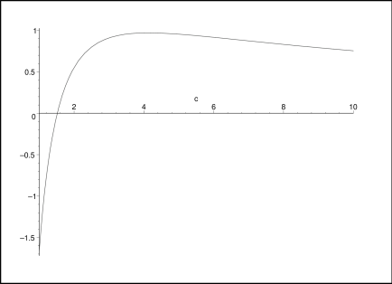
Figure 1: Coordinate $z_{max}$ as a function of $c$.

One can see that the root is the unique one. The analytical proof can be found below but it requires another representation.

One can see that for $c<3$ the dependence $z_{max}(c)$ is a growing function. But for $c>(6\exp(1))^{1/4}$ already the first iteration for spectrum has positive maximum. Since the maximum of precise solution can not be lower than the maximum of precise solution. The maximum of precise solution has to be positive. But the precise solution can not lie higher than $cx$. So, it must have maximum at positive $x$. It means that the slow decrease of $z_{max}(c)$ which is seen in the figure, can not lead to the negative $z_{max}$.

So, the solution of the problem A is also the unique one.

5 Iterated equation

5.1 Some properties of solution of the iterated equation

For further purposes it will be necessary to investigate the iterated equation and to show the properties of solution. The iterated equation will be written in the following form

$$\tilde{g}(z)=\int_{-\infty}^{z}(z-x)^{3}\exp(cx-\int_{-\infty}^{x}(x-y)^{3}\exp(cy-\tilde{g}(y))dy)dx$$ (9)

One can see the following property

The solution of (9) is so, that the spectrum, i.e. the function

$$\tilde{\psi}=\exp(cx-\tilde{g})$$

has only one maximum.

Really, $\tilde{g}$ is the integral with the positive sub-integral function. The function $d\tilde{g}/dz$ can be presented as

$$\frac{d\tilde{g}(z)}{dz}=3\int_{-\infty}^{z}(z-x)^{2}\exp(cx-\int_{-\infty}^{x}(x-y)^{3}\exp(cy-\tilde{g}(y))dy)dx$$

It is also the integral with the positive sub-integral function. Then the function $d\tilde{g}/dz$ is also positive.

Now we recall functions

$$g_{0}=0$$

$$g_{1}=\frac{6}{c^{4}}\exp(cx)$$

$$g_{2}=\int_{-\infty}^{z}(z-x)^{3}\exp(cx-\frac{6}{c^{4}}\exp(cx))dx$$

They are simply the already constructed iterations for eq. (5).

One can easily see that every solution of (9) has to satisfy

$$g_{2}\leq\tilde{g}\leq g_{1}$$

The proof is simply the comparison between expressions for $g_{1}$, $g_{2}$ and the iterated equation.

5.2 The uniqueness of the solution of the iterated equation at small $z$

Here one has to fulfill two procedures:

1. To construct iterations to see the existence of solution

2. To construct estimates for different solutions to see the uniqueness

These procedures have similar technical realization. This is the reason why here we restrict the consideration only by the second case. The first case is identical in ideology to the procedure used for original (not iterated) equation. There we solved only the first problem. The second case for the original (non iterated) solution can be solved as it is described here.

Actually the existence for the iterated solution is already proven as the limit of increasing sequence (odd iterations) restricted from above and the limit of decreasing sequence (even iterations) restricted from below.

The proof is the following:

Suppose that $\tilde{g}$ and $\tilde{q}$ are two different solutions of equation (9). Then

$$\tilde{g}(z)-\tilde{q}(z)=\int_{-\infty}^{z}(z-x)^{3}[\exp(cx-\int_{-\infty}^{x}(x-y)^{3}$$

$$\exp(cy-\tilde{g}(y))dy)-\exp(cx-\int_{-\infty}^{x}(x-y)^{3}\exp(cy-\tilde{q}(y))dy)]dx$$

We shall formally denote the initial functions as $\tilde{g}_{0}$ and $\tilde{q}_{0}$ and determine the ”formal iterations” $\tilde{g}_{i}$ and $\tilde{q}_{i}$ as

$$\tilde{g}_{i+1}(z)=\int_{-\infty}^{z}(z-x)^{3}\exp(cx-\int_{-\infty}^{x}(x-y)^{3}\exp(cy-\tilde{g}_{i}(y))dy)dx$$

$$\tilde{q}_{i+1}(z)=\int_{-\infty}^{z}(z-x)^{3}\exp(cx-\int_{-\infty}^{x}(x-y)^{3}\exp(cy-\tilde{q}_{i}(y))dy)dx$$

Then we have

$$\tilde{g}_{i+1}(z)-\tilde{q}_{i+1}(z)=\int_{-\infty}^{z}(z-x)^{3}[\exp(cx-\int_{-\infty}^{x}(x-y)^{3}$$

$$\exp(cy-\tilde{g}_{i}(y))dy)-\exp(cx-\int_{-\infty}^{x}(x-y)^{3}\exp(cy-\tilde{q}_{i}(y))dy)]dx$$

We consider $z\leq z_{in}$. Recall that $z_{in}$ is chosen from condition

$$\frac{6}{c^{4}}\exp(cz_{in})=1-\epsilon$$

with a small positive $\epsilon$.

We see that

$$z_{in}\leq z\leq x\leq y$$

One can reorganize the previous equation as

$$\tilde{g}_{i+1}(z)-\tilde{q}_{i+1}(z)=\int_{-\infty}^{z}(z-x)^{3}\exp(cx)[\exp(-\int_{-\infty}^{x}(x-y)^{3}\exp(cy-\tilde{g}_{i}(y))dy)-$$

$$\exp(-\int_{-\infty}^{x}(x-y)^{3}\exp(cy-\tilde{q}_{i}(y))dy)]dx$$

Then

$$|\tilde{g}_{i+1}(z)-\tilde{q}_{i+1}(z)|\leq\int_{-\infty}^{z}(z-x)^{3}\exp(cx)|\exp(-\int_{-\infty}^{x}(x-y)^{3}\exp(cy-\tilde{g}_{i}(y))dy)-$$

$$\exp(-\int_{-\infty}^{x}(x-y)^{3}\exp(cy-\tilde{q}_{i}(y))dy)|dx$$

Since for positive $\alpha_{1}$, $\alpha_{2}$ one can see that

$$|\exp(-\alpha_{1})-\exp(-\alpha_{2})|\leq|\alpha_{1}-\alpha_{2}|$$

and $\int_{-\infty}^{x}(x-y)^{3}\exp(cy-\tilde{g}_{i}(y))dy$, $\int_{-\infty}^{x}(x-y)^{3}\exp(cy-\tilde{q}_{i}(y))dy$ are evidently positive then

$$|\exp(-\int_{-\infty}^{x}(x-y)^{3}\exp(cy-\tilde{g}_{i}(y))dy)-\exp(-\int_{-\infty}^{x}(x-y)^{3}\exp(cy-\tilde{q}_{i}(y))dy)|\leq$$

$$|\int_{-\infty}^{x}(x-y)^{3}\exp(cy-\tilde{g}_{i}(y))dy)-\int_{-\infty}^{x}(x-y)^{3}\exp(cy-\tilde{q}_{i}(y))dy)|$$

Having rearranged the r.h.s. we come to

$$|\exp(-\int_{-\infty}^{x}(x-y)^{3}\exp(cy-\tilde{g}_{i}(y))dy)-\exp(-\int_{-\infty}^{x}(x-y)^{3}\exp(cy-\tilde{q}_{i}(y))dy)|\leq$$

$$\int_{-\infty}^{x}(x-y)^{3}\exp(cy)|\exp(-\tilde{g}_{i}(y))-\exp(-\tilde{q}_{i}(y))|dy$$

Since $\tilde{q}_{i}(y)\geq 0$, $\tilde{q}_{i}(y)\geq 0$, one can see that

$$|\exp(-\tilde{g}_{i}(y))dy)-\exp(-\tilde{q}_{i}(y))dy)|\leq$$

$$|\tilde{g}_{i}(y)-\tilde{q}_{i}(y)|$$

and then

$$|\exp(-\int_{-\infty}^{x}(x-y)^{3}\exp(cy-\tilde{g}_{i}(y))dy)-\exp(-\int_{-\infty}^{x}(x-y)^{3}\exp(cy-\tilde{q}_{i}(y))dy)|\leq$$

$$\int_{-\infty}^{x}(x-y)^{3}\exp(cy)|\tilde{g}_{i}(y)-\tilde{q}_{i}(y)|dy$$

Then for the norm in $C$ space one can write

$$|\exp(-\int_{-\infty}^{x}(x-y)^{3}\exp(cy-\tilde{g}_{i}(y))dy)-\exp(-\int_{-\infty}^{x}(x-y)^{3}\exp(cy-\tilde{q}_{i}(y))dy)|\leq$$

$$\int_{-\infty}^{x}(x-y)^{3}\exp(cy)dy||\tilde{g}_{i}(y)-\tilde{q}_{i}(y)||$$

Having calculated the integral one comes to

$$|\exp(-\int_{-\infty}^{x}(x-y)^{3}\exp(cy-\tilde{g}_{i}(y))dy)-\exp(-\int_{-\infty}^{x}(x-y)^{3}\exp(cy-\tilde{q}_{i}(y))dy)|\leq$$

$$(1-\epsilon)||\tilde{g}_{i}(y)-\tilde{q}_{i}(y)||$$

Now we shall estimate $|\tilde{g}_{i+1}-\tilde{q}_{i+1}|$. We have

$$|\tilde{g}_{i+1}-\tilde{q}_{i+1}|\leq\int_{-\infty}^{z}(z-x)^{3}\exp(cx)(1-\epsilon)||\tilde{g}_{i}(y)-\tilde{q}_{i}(y)||dx$$

and then

$$|\tilde{g}_{i+1}-\tilde{q}_{i+1}|\leq(1-\epsilon)^{2}||\tilde{g}_{i}(y)-\tilde{q}_{i}(y)||$$

We can apply this recurrent procedure several times and come to

$$|\tilde{g}_{i+1}-\tilde{q}_{i+1}|\leq(1-\epsilon)^{2i}||\tilde{g}_{0}(y)-\tilde{q}_{0}(y)||$$

So, we see that $|\tilde{g}_{i+1}-\tilde{q}_{i+1}|$ can be estimated by some positive members of geometric progression. So, it means that this sequence converges and the limit is the real unique solution. The difference between $\tilde{g}_{i}$ and $\tilde{q}_{i}$ can be made negligibly small.

So, we conclude that $\tilde{g}$ and $\tilde{q}$ is actually one solution. The uniqueness is proven. The existence can be proven by construction of Caushi sequence.

5.3 Further properties of solution

We need some estimates for $\tilde{\psi}=\exp(cx-\tilde{g})$.

Having constructed

$$\tilde{\xi}_{i}=cx-\tilde{g}_{i}$$

$$\tilde{\xi}=cx-\tilde{g}$$

we see that

$$cx-g_{1}\leq\tilde{\xi}_{i}\leq cx-g_{2}$$

$$cx-g_{1}\leq\tilde{\xi}\leq cx-g_{2}$$

Then it follows that

$$max\tilde{\xi}_{i}\leq max(cx-g_{2})$$

$$max\tilde{\xi}_{i}\geq max(cx-g_{1})$$

$$max\tilde{\xi}\leq max(cx-g_{2})$$

$$max\tilde{\xi}\geq max(cx-g_{1})$$

and we have the estimates for the maximum.

We introduce $z_{21}$ as to satisfy

$$(cx-g_{2})|_{z_{21}}=max\{cx-g_{1}\}$$

There are two $z_{21}$. We shall note them $z_{21l}$ and $z_{21r}$ and choose to have $z_{21l}<z_{21r}$.

One can easily see that

$$z_{21l}<\tilde{z}_{max\ i}<z_{21r}$$

where $\tilde{z}_{max\ i}$ is the point where the maximum of $\tilde{\xi}_{i}$ is attained. It is also clear that

$$z_{@1l}<\tilde{z}_{max}<z_{21r}$$

where $\tilde{z}_{max}$ is the point where the maximum of $\tilde{\xi}$ is attained.

So, now the natural boundary $z_{21r}$ appeared and we shall consider $z<z_{21r}$.

Since to solve the problem of existence we have to construct iterations then the estimates for iterations are presented.

5.4 Uniqueness for intermediate $z$

Suppose that there are two different solutions $\tilde{g}$ and $\tilde{q}$. According to the previous constructions they must coincide at $z<z_{in}$. Then

$$\tilde{g}(z)-\tilde{q}(z)=\int_{z_{in}}^{z}(z-x)^{3}[\exp(cx-\int_{-\infty}^{x}(x-y)^{3}$$

$$\exp(cy-\tilde{g}(y))dy)-\exp(cx-\int_{-\infty}^{x}(x-y)^{3}\exp(cy-\tilde{q}(y))dy)]dx$$

Then for the absolute values

$$|\tilde{g}(z)-\tilde{q}(z)|\leq\int_{z_{in}}^{z}(z-x)^{3}|\exp(cx-\int_{-\infty}^{x}(x-y)^{3}$$

$$\exp(cy-\tilde{g}(y))dy)-\exp(cx-\int_{-\infty}^{x}(x-y)^{3}\exp(cy-\tilde{q}(y))dy)|dx$$

Then since $z-x\leq z-z_{in}$ we come to

$$|\tilde{g}(z)-\tilde{q}(z)|\leq(z-z_{in})^{3}\int_{z_{in}}^{z}|\exp(cx-\int_{-\infty}^{x}(x-y)^{3}$$

$$\exp(cy-\tilde{g}(y))dy)-\exp(cx-\int_{-\infty}^{x}(x-y)^{3}\exp(cy-\tilde{q}(y))dy)|dx$$

The function

$$|\exp(cx-\int_{-\infty}^{x}(x-y)^{3}\exp(cy-\tilde{g}(y))dy)-\exp(cx-\int_{-\infty}^{x}(x-y)^{3}\exp(cy-\tilde{q}(y))dy)|$$

can be estimated as

$$|\exp(cx-\int_{-\infty}^{x}(x-y)^{3}\exp(cy-\tilde{g}(y))dy)-\exp(cx-\int_{-\infty}^{x}(x-y)^{3}\exp(cy-\tilde{q}(y))dy)|\leq$$

$$\exp(cz_{21r})|\exp(-\int_{-\infty}^{x}(x-y)^{3}\exp(cy-\tilde{g}(y))dy)-\exp(-\int_{-\infty}^{x}(x-y)^{3}\exp(cy-\tilde{q}(y))dy)|$$

Since both

$$\int_{-\infty}^{x}(x-y)^{3}\exp(cy-\tilde{q}(y))dy>0$$

and

$$\int_{-\infty}^{x}(x-y)^{3}\exp(cy-\tilde{q}(y))dy>0$$

are positive then

$$|\exp(-\int_{-\infty}^{x}(x-y)^{3}\exp(cy-\tilde{g}(y))dy)-\exp(-\int_{-\infty}^{x}(x-y)^{3}\exp(cy-\tilde{q}(y))dy)|\leq$$

$$|\int_{-\infty}^{x}(x-y)^{3}\exp(cy-\tilde{g}(y))dy-\int_{-\infty}^{x}(x-y)^{3}\exp(cy-\tilde{q}(y))dy|$$

The last function allows the estimate

$$|\int_{-\infty}^{x}(x-y)^{3}\exp(cy-\tilde{g}(y))dy-\int_{-\infty}^{x}(x-y)^{3}\exp(cy-\tilde{q}(y))dy|\leq$$

$$|\int_{-\infty}^{x}(z_{21r}-z_{in})^{3}[\exp(cy-\tilde{g}(y))-\exp(cy-\tilde{q}(y))]dy|$$

Since $g$ and $q$ are positive we come to

$$|\int_{-\infty}^{x}(z_{21r}-z_{in})^{3}[\exp(cy-\tilde{g}(y))-\exp(cy-\tilde{q}(y))]dy|\leq$$

$$(z_{21r}-z_{in})^{3}\exp(cz_{21r})|\int_{-\infty}^{x}[\tilde{g}(y)-\tilde{q}(y)]dy|$$

The final inequality will be

$$\int_{-\infty}^{x}[\tilde{g}(y)-\tilde{q}(y)]dy\leq||q-g||(x-z_{in})$$

As the result we come to

$$|g-q|\leq(z_{21r}-z_{in})^{3}\exp(cz_{21r})||g-q||(z-z_{in})^{3}\int_{z_{in}}^{z}(x-z_{in})dx$$

Having marked that $(z-z_{in})<(z_{21r}-z_{in})$ and $(x-z_{in})<(z_{21r}-z_{in})$ we see that

$$||g-q||\leq(z_{21r}-z_{in})^{7}\exp(cz_{21r})||g-q||(z-z_{in})$$

Now we can formally organize sequential application of the last estimate and having applied the last relation $i$ times with explicit integration of $(z-z_{in})$ we get

$$||g-q||\leq(z_{21r}-z_{in})^{7}\exp(cz_{21r})||g-q||(z-z_{in})^{i}/i!$$

One can easily see that the last r.h.s. is the term in the Taylor’s expansion of

$$(z_{21r}-z_{in})^{7}\exp(cz_{21r})||g-q||\exp(z-z_{in})$$

with all standard consequences mentioned above in such a situation.

The uniqueness for $z<z_{21r}$ is proven.

In principle it is sufficient for all finite $z_{21r}$. But below more fine estimates will be proven.

5.5 Uniqueness for the big values of arguments

Here we shall use the function $\xi$ or $\varphi$ instead of $cx-g$. Again we mark by ”$\tilde{}$” the solution referred to the iterated equation.

To prove uniqueness for $z>z_{21r}$ one can note that

$$\exp(cx-\int_{-\infty}^{x}(x-y)^{3}\exp(\tilde{\xi})dy)\leq\exp(\xi_{2})<max\exp(\xi_{2})$$

Then it is clear that

$$\exp(cx-\int_{-\infty}^{x}(x-y)^{3}\exp(\tilde{\xi})dy)\leq R|cx-\int_{-\infty}^{x}(x-y)^{3}\exp(\tilde{\xi})dy|$$

with some fixed constant $R$. This already solves all problems. But we shall present a detailed derivation.

One can also note that the previous consideration will be valid not only for $z_{21r}$ but for any finite $z$. For such a value $z_{21r}$ we shall choose $z$ or $x$ at which already

$$cx-\int_{-\infty}^{x}(x-y)^{3}\exp(\tilde{\xi})dy<0$$

Since one can prove that $cx-\int_{-\infty}^{x}(x-y)^{3}\exp(\tilde{\xi})dy$ goes to $-\infty$ at big $z$ the last requirement could be satisfied.

Let us suppose that there are two different solutions. For two different solutions $\tilde{\xi}$ and $\tilde{\varphi}$ one can write

$$|\tilde{\varphi}-\tilde{\xi}|\leq\int_{-\infty}^{z}(z-x)^{3}|(-cx+\int_{-\infty}^{x}(x-y)^{3}\exp(\tilde{\varphi})dy)-$$

$$(-cx+\int_{-\infty}^{x}(x-y)^{3}\exp(\tilde{\xi})dy)|dx$$

We can rewrite the last equation as

$$|\tilde{\varphi}-\tilde{\xi}|\leq\int_{-\infty}^{z}(z-x)^{3}\int_{-\infty}^{x}(x-y)^{3}|\exp(\tilde{\varphi})-\exp(\tilde{\xi})|dydx$$

Since at $z<z_{21r}$ the solution is unique then $\tilde{\varphi}=\tilde{\xi}$ and we cut the lower limit of integration up to $z_{21r}$. Then

$$|\tilde{\varphi}-\tilde{\xi}|\leq\int_{z_{21r}}^{z}(z-x)^{3}\int_{z_{21r}}^{x}(x-y)^{3}|\exp(\tilde{\varphi})-\exp(\tilde{\xi})|dydx$$

Since it is known that both $\tilde{\varphi}$ and $\tilde{\xi}$ have only one maximum and decrease at $|z|\rightarrow\infty$ it is clear that both $\tilde{\varphi}$ and $\tilde{\xi}$ are less than some constant and then

$$|\exp(\tilde{\varphi})-\exp(\tilde{\xi})|\leq Q|\tilde{\varphi}-\tilde{\xi}|$$

with some fixed constant $Q$. Then

$$|\tilde{\varphi}-\tilde{\xi}|\leq Q\int_{z_{21r}}^{z}(z-x)^{3}\int_{z_{21r}}^{x}(x-y)^{3}|\tilde{\varphi}-\tilde{\xi}|dydx$$

and

$$||\tilde{\varphi}-\tilde{\xi}||\leq Q\int_{z_{21r}}^{z}(z-x)^{3}\int_{z_{21r}}^{x}(x-y)^{3}dydx||\tilde{\varphi}-\tilde{\xi}||$$

The chain of inequalities can be prolonged

$$||\tilde{\varphi}-\tilde{\xi}||\leq Q\int_{z_{21r}}^{z}(z-x)^{3}\int_{z_{21r}}^{x}(z-y)^{3}dydx||\tilde{\varphi}-\tilde{\xi}||$$

The r.h.s. can be rewritten in a following way

$$||\tilde{\varphi}-\tilde{\xi}||\leq Q(\int_{z_{21r}}^{z}(z-x)^{3}dx)^{2}||\tilde{\varphi}-\tilde{\xi}||$$

Then since $(z-x)<(z-z_{21r})$ one can see that

$$||\tilde{\varphi}-\tilde{\xi}||\leq Q(\int_{z_{21r}}^{z}(z-z_{21r})^{3}dx)^{2}||\tilde{\varphi}-\tilde{\xi}||$$

In other regimes of vapor consumption it is important to prove the uniqueness for the arbitrary positive power $\alpha$ instead of $3$. So, we get the following inequality

$$||\tilde{\varphi}-\tilde{\xi}||\leq Q(\int_{z_{21r}}^{z}(z-z_{21r})^{\alpha}dx)^{2}||\tilde{\varphi}-\tilde{\xi}||$$

Having calculated the integral we come to

$$||\tilde{\varphi}-\tilde{\xi}||\leq Q(z-z_{21r})^{2\alpha+2}||\tilde{\varphi}-\tilde{\xi}||$$

Now we apply this inequality $i$ times with explicit integration of $(z-z_{21r})$ and the result of this integration. Finally we get

$$||\tilde{\varphi}-\tilde{\xi}||\leq RQ\frac{(z-z_{21r})^{W(i)}}{V(i)}||\tilde{\varphi}_{0}-\tilde{\xi}_{0}||$$

where $\tilde{\varphi}_{0}$ and $\tilde{\xi}_{0}$ are initial approximations. For functions $V$ and $W$ one can get some estimates

$$V(i)>i!$$

$$W(i)<(2[\alpha]+2)i+const_{1}$$

where $[\alpha]$ is the minimal integer number greater than $\alpha$ and $const_{1}$ is some constant which is independent on $i$.

Now we can make the following remark: We can assume that earlier we proved the uniqueness until $z_{21r}+1$. Then $z-z_{21r}>1$.

Then we come to the following estimate

$$||\tilde{\varphi}-\tilde{\xi}||\leq constQ\frac{(z-z_{21r})^{(2[\alpha]+2)i}}{i!}(z-z_{21r})^{const_{1}}$$

One can see that the r.h.s. is the member of the Taylor’s serial for the function

$$Qconst(z-z_{21r})^{const_{1}}\exp((z-z_{21r})^{(2[\alpha]+2)})$$

So, then the conclusion about the uniqueness and existence of solution can be also proven.

6 $f$-representation

One can rewrite the equation (5) by the substitution

$$x\rightarrow cx$$

$$z\rightarrow cz$$

in a following form

$$g(z)=f\int_{-\infty}^{z}(z-x)^{3}\exp(x-g(x))dx$$

with $f=c^{-4}$.

This representation is more convenient to show the uniqueness of dependence of $z_{max}$ on $c$.

Suppose that the are two parameters $f_{1}$ and $f_{2}$. Let it be $f_{2}>f_{1}$.

Then

$$g_{f_{1}}(z)=f_{1}\int_{-\infty}^{z}(z-x)^{3}\exp(x-g_{f_{1}}(x))dx$$

$$g_{f_{2}}(z)=f_{2}\int_{-\infty}^{z}(z-x)^{3}\exp(x-g_{f_{2}}(x))dx$$

For $g_{f_{2}}$ we construct iterations with initial approximation

$$g_{f_{2}\ 0}(x)=g_{f_{1}}(x)$$

and a recurrent procedure

$$g_{f_{2}\ i+1}(z)=f_{2}\int_{-\infty}^{z}(z-x)^{3}\exp(x-g_{f_{2}\ i}(x))dx$$

Then

$$g_{f_{2}\ 1}(z)=f_{2}\int_{-\infty}^{z}(z-x)^{3}\exp(x-g_{f_{1}}(x))dx=(f_{2}/f_{1})g_{f_{1}}(x)$$

So,

$$g_{f_{2}\ 1}(z)>g_{f_{1}}(x)(1+\epsilon)$$

with finite positive small $\epsilon$.

One can see the following important fact

The following formula

$$\frac{d|g_{f_{2}\ 1}-g_{f_{2}\ 0}|}{dz}>0$$

takes place.

This is clear if one notes that

$$(f_{2}-f_{1})\int_{-\infty}^{z}(z-x)^{3}\exp(x-g_{f_{1}\ i}(x))dx$$

grows when $z$ grows.

Really

$$3(f_{2}-f_{1})\int_{-\infty}^{z}(z-x)^{2}\exp(x-g_{f_{1}\ i}(x))dx>0$$

This proves the inequality.

One can also prove the following statement:

There exists a point $z`_{in}$ until which $g_{f2\ 2}>g_{f2\ 0}$

This follows from the explicit estimates for the first and the second iterations with zero initial approximations. It is known that at $z\rightarrow-\infty$ they come very close and estimate the solution very precise. Really,

$$g_{f_{1}}\rightarrow g_{f_{1}\ as}\sim 6f_{1}\frac{\exp(cx)}{c^{4}}=6f_{1}\exp(x)$$

$$g_{f_{2}}\rightarrow g_{f_{2}\ as}\sim 6f_{2}\frac{\exp(cx)}{c^{4}}=6f_{2}\exp(x)$$

Then

$$g_{f_{2}\ 2\ as}=g_{f_{2}\ 1\ as}=g_{f_{2}\ as}$$

Since

$$g_{f_{2}\ 1\ as}>g_{f_{2}\ 0}=g_{f_{1}}$$

we see that asymptotically

$$g_{f_{2}\ 2}>g_{f_{2}\ 0}$$

Then the necessary point exists. This proves the statement.

As the result we see that at extremely big negative $z$ the following hierarchy takes place

$$g_{f2\ 0}\leq g_{f2\ 2}\leq...\leq g_{f2\ 3}\leq g_{f2\ 1}$$

So, all of them are between $g_{f2\ 0}$ and $g_{f2\ 1}$ at extremely big negative $z$. Later iterations can go away from this frames. We shall mark the coordinate when iteration number $i$ attains the mentioned boundary by $z`_{i}$.

One can easily see that either $z`_{i}$ goes to infinity or $z`_{i}$ exists. One can also see that

$$z`_{i+1}\geq z`_{i}$$

It is easy to see because the integration is going only for the values of argument smaller than the current one. This proves the estimate.

A question appears whether the limit

$$\lim_{i\rightarrow\infty}z`_{i}$$

exists.

The existence of a limit means that at this limiting point (let it be $z`_{\infty}$) the limit of odd iterations differs from the limit of even iterations. But both the limit of odd iterations and the limit of even iterations belong to the solutions of the iterated equation. But we have already proved that the solution of the iterated equation is the unique one. So, the contradiction is evident. We come to the conclusion that there is no such a limit.

The last conclusion particularly means that

$$g_{f_{2}}>g_{f_{1}}$$

Really, the analogous reasons show that the possible points of crossing $g_{f_{1}\ 2j+2}$, $g_{f_{1}\ 2j+4}$, etc. with $g_{f_{1}\ 2j}$ for every $j$ cannot have a finite limit. So, for every finite $z$ we see that

$$g_{f_{2}}>g_{f_{2}\ 2j}$$

Since for every finite $z$ there is such $j$ which provides

$$g_{f_{2}\ 2j}>g_{f_{2}\ 0}=g_{f_{1}}$$

we see that

$$g_{f_{2}}>g_{f_{1}}$$

This proves the necessary inequality.

The last inequality leads to the important relation

$$\frac{dg_{f}}{df}>0$$

for any given value of the argument.

7 The uniqueness of the root

We analyze the question: how many solutions with different $c$ (or $f$) can have the maximum of $cx-g$ (or $x-g_{f}$) at $x=0$?

The most evident answer is that there will be only one solution but this has to be proven. To prove it we shall use $f$-representation.

The equation for the coordinate $z_{max}$ of the spectrum will be the following

$$1=3f\int_{-\infty}^{z_{max}}(z_{max}-x)^{2}\exp(x-g(x))dx$$

Then

$$f=\frac{1}{3}(\int_{-\infty}^{z_{max}}(z_{max}-x)^{2}\exp(x-g(x))dx)^{-1}$$

Now we can calculate $df/dz_{max}$ Then we shall take it at $z_{max}=0$ and if we are able to prove that $df/dz_{max}<0$ then the necessary property will be established.

The possibility to take here $z_{max}=0$ is ensured by existence of the root which was proven a few sections earlier. Now we see that the proof of existence of the root was really necessary.

For the derivative $df/dz_{max}$ one can get the following equation

$$\frac{df}{dz_{max}}=-\frac{1}{3}(\int_{-\infty}^{z_{max}}(z_{max}-x)^{2}\exp(x-g(x))dx)^{-2}Y$$

where

$$Y=\frac{d\int_{-\infty}^{z_{max}}(z_{max}-x)^{2}\exp(x-g(x))dx}{dz_{max}}$$

The direct calculation gives

$$Y=2\int_{-\infty}^{z_{max}}(z_{max}-x)\exp(x-g(x))dx-\int_{-\infty}^{z_{max}}(z_{max}-x)^{2}\exp(x-g(x))\frac{dg}{df}dx$$

In the last relation one has to consider $\frac{dg}{df}$ as a function of $x$.

One can also get for $Y(0)$ the following equation

$$Y(0)=\frac{1}{3}\frac{d^{2}g}{dz^{2}}|_{z=0}-\int_{-\infty}^{0}x^{2}\exp(x-g(x))\frac{dg}{df}dx$$

Now we shall calculate $dg/df$. One can get the following equation

$$\frac{dg}{df}=\int_{-\infty}^{x}(x-y)^{3}\exp(y-g(y))dy-f\int_{-\infty}^{x}(x-y)^{3}\exp(y-g(y))\frac{dg}{df}dy$$

One can rewrite the last relation as

$$\frac{dg}{df}=g/f-f\int_{-\infty}^{x}(x-y)^{3}\exp(y-g(y))\frac{dg}{df}dy$$

Since $dg/df>0$ (it has been already proven) then the sub-integral function $(x-y)^{3}\exp(y-g(y))\frac{dg}{df}$ is positive and the we have

$$f\int_{-\infty}^{x}(x-y)^{3}\exp(y-g(y))\frac{dg}{df}dy\geq 0$$

Then

$$0\leq\frac{dg}{df}\leq g/f$$

Now we shall return to the function $Y$. One can rewrite it as

$$Y(z_{max})=\int_{-\infty}^{z_{max}}(z_{max}-x)[2-(z_{max}-x)\frac{dg}{df}]\exp(x-g(x))dx$$

Then

$$Y(0)=\int_{-\infty}^{0}(0-x)[2-(0-x)\frac{dg}{df}]\exp(x-g(x))dx$$

The sign of $Y(0)$ is important.

Then we consider the function

$$l=[2+x\frac{dg}{df}]$$

We have to recall that $x$ takes here only negative values.

Then

$$l>[2+x\frac{g}{f}]$$

For $g$ one can take the estimate

$$g<f\exp(x)$$

going from the first iteration with initial zero approximation. Then

$$l>[2+x\exp(x)]$$

One can easily see that the function $x\exp(x)$ has only one minimum at $x=-1$ where this function is $-\exp(-1)$.

Then

$$l>2-exp(-1)>0$$

Then $Y(0)>0$ and

$$df/dz_{max}|_{z_{max}=0}<0$$

It means that the uniqueness of the root is proven.

8 Uniqueness of solution of the problem B

Suppose that $\xi_{1}$ and $\xi_{2}$ are two different solutions of the problem B. Then (this is the statement)

$$\int_{-\infty}^{0}y^{2}\exp(-\xi_{1}(y))dy=\int_{-\infty}^{0}y^{2}\exp(-\xi_{2}(y))dy$$

We shall prove this equality.

Suppose that these integrals do not equal, let it be

$$\int_{-\infty}^{0}y^{2}\exp(-\xi_{1}(y))dy>\int_{-\infty}^{0}y^{2}\exp(-\xi_{2}(y))dy$$

Then for the problem A one can see that $c_{1}>c_{2}$ and $f_{1}<f_{2}$. Then (because there is only one root of equation $z_{max}(f)=0$) we come to the conclusion that at least one solution can not have maximum of $x-g_{f}(x)$ at $z=0$. So, at least one solution is not a solution of the problem B.

We come to the contradiction.

This completes the proof.

We can formulate another statement:

The solution of the problem B is unique.

It is clear because as it is proven

$$\int_{-\infty}^{0}y^{2}\exp(-\xi_{2}(y))dy$$

has one fixed value. Then it is the problem of solution of equation (5) with fixed $c$. The last problem has the unique solution.

This completes the justification of the uniqueness of solution of the problem B.

One can also see that the solution of the problem A is the solution of the problem B.

To see this one can simply differentiate the solution and then use the condition for derivative.

Since the solution of the problem A is unique and solution of the problem B is unique one can easily see that:

The solution of the problem A and the problem B coincide.

9 Similarity of the forms of the size distributions

Having established the uniqueness of solution of equation (5) with given $c$ (or $f$), the uniqueness of the solution of the problem A and the uniqueness of the solution of the problem B we can investigate the correspondence between solutions with different $c$.

The main result will be the following:

Actually all solutions of equation (5) with different $c$ (or $f$) are identical.

Really, in equation (5) we fulfill the substitution

$$zc\rightarrow z$$

$$xc\rightarrow x$$

and come to

$$g(z)=\frac{1}{c^{4}}\int_{-\infty}^{z}(z-x)^{3}\exp(x-g(x))dx$$

The next transformation will be the shift

$$z\rightarrow z+\Delta$$

$$x\rightarrow x+\Delta$$

We choose

$$\Delta\sim 4\ln c$$

The factor $(z-x)$ can not change. the region of integration will be actually the same - from infinity up to a ”current moment” $z$.

Then the amplitude $1/c^{4}$ can be easily canceled.

So, the spectrum, i.e. the function

$$\Phi=\exp(x-g)$$

has one and same form, which differs only by rescaling of the argument and the rescaling of the amplitude. The numerical simulations confirm this conclusion (see the figure 2)

Figure 2: Forms of distributions (with the shifts -0.05; 0; +0.05 for $c=0.1;1;10$

The shift in these pictures was introduced only in order to see three curves. When the shift will be zero then only one curve can be seen. The coincidence is practically ideal.

The certain question whether there can be simply multiple repeating of solutions appears here. But the uniqueness of solution of equation (5) with given $c$ and the property $dg/df>0$ established earlier ensure the absence of such repeating.

References

- [1] Kurasov V., Physical Review E, vol.49, p.3948 (1994)
- [2] Kurasov V., Physica A, vol. 226, p.117 (1996)