Reconstruction of condensed magnetoexciton droplet in a trap in strong magnetic fields

Abstract

We investigate theoretically the Bose-Einstein condensation of trapped magnetoexcitons in a two-layered system with one layer containing electrons and the other layer containing holes. We have studied the spatial variations of the condensate density in the droplet of electrons and holes. We find that the shape of the electron and hole densities may change due to the competition between repulsive electron-electron/hole-hole interaction and confinement potential of the trap. Our mean field calculations show that when the confinement strength is strong enough the condensate density is peaked at the edge of the droplet, and as the confinement strength weakens the condensate density displays one inner peak and another peak at the edge. For much weaker confinement potential the condensate density may display one broad peak.

I Introduction

The Bose-Einstein condensation (BEC) of excitons is more likely to occur when (a) electrons and holes are spatially separated, (b) a strong magnetic field is present, and (c) bosons are confined in a trap. When electrons and holes are spatially separated exciton lifetime increases. The lifetime depends on the wavefunction overlap between electrons and holes. In coupled quantum wells the wavefunction overlap can be controlled by an external electric field applied perpendicular to the quantum wells. It was shown theoretically that in such a system excitonic condensate can be realized in strong magnetic fields nearly at all filling factors when the separation between the electron and hole layers is less than the magnetic length YM . Only for large separations fractional quantum Hall states or Wigner crystal states may be realized. Different aspects of excitonic BEC in two dimensional systems in strong magnetic fields have been investigated over the yearsKH ; paquet ; kor ; mos ; LY ; YF ; BR ; YM ; butov ; Chen ; Ber . As the observation of atomic BEC demonstrates wieman the conditions for BEC are improved if bosons are confined in a trap. Several groups have recently investigated excitonic BEC in a trap in the absence of a magnetic field. Experimentally the possibility of excitonic BEC was explored in traps of double quantum wells neg ; Butov ; Snoke . Theoretically exciton BEC in a trap was investigated in a mean field theory including electron-electron and hole-hole interactionszhu . Signatures of BEC in angular distribution of photoluminescence have been also explored theoreticallyKee .

In this paper we investigate theoretically the BEC of excitons when both a strong magnetic field and a trap are present in double quantum wells. The magnetic field is applied perpendicular to the layers and the confinement potential traps particles laterally, i. e. in the layers. We consider the strong magnetic field limit where only the states in the lowest Landau level are relevant. The trap potential will split the degenerate lowest Landau level states. What is interesting about strong magnetic field limit is that the particle density cannot exceed a certain value $1/2\pi\ell^{2}$, where $\ell$ is the magnetic length. In bulk 2D this density is achieved when the lowest Landau level if completely filled, i. e. when the Landau level filling factor is one. A strong confinement potential pushes particles in each layer to the center of the potential and the particle density takes the largest possible value except near the edge of such a droplet. Similar effect is not present in the absence of a strong magnetic field. We will call this state the maximum density droplet (MDD). When the confinement potential becomes weaker the particle density can take a smaller value at some place in the droplet. Such a reconstruction for MDD Yang1 ; Yang2 ; Yang3 in electron single dots was investigated both theoretically and experimentally by several groups in strong magnetic fields Yang1 ; Yang2 ; Yang3 ; As ; Oo ; Kl ; So ; Re ; Ch ; Ka . The purpose of this paper is to investigate how a reconstruction of the MDD affects the condensed magnetoexcitons.

We have explored this problem within a BCS theory. In the MDD condensed magnetoexcitons are found near the edge of the droplet, see Fig. 2. We find that as the strength of the confinement potential weakens this MDD becomes unstable and density depletion starts to occur at the interior of the droplet. In this state condensed magnetoexcitons are found both in the interior of the droplet and near the edge of the droplet, see Fig.3. When the confinement potential is weakened further the density depletion of electrons and holes increases. This behavior is similar to how the electron MDD reconstructs in electron single dots Yang3 . However, we find that, unlike the electron single dot case, where the number of electrons depleted increases discontinuously from one, two, and etc., Yang3 , the density depletion increases continuously with the decrease in the strength of the confinement potential. When density changes from the uniform state are more severe the order parameter may display one broad peak.

This paper is organized as follows. In Sec.II we describe our model and its Hamiltonian. A gap equation for the condensate is derived in Sec.III. In Sec.IV we show solutions of this gap equation. Conclusions are given in Sec.V.

II Model

An artificial trap for excitons in double quantum wells can be set up by changing locally the well width on one side of double quantum well zhu . An in-plane random potential may also provide a local potential minimum which can host electrons and holesButov ; Snoke . A parabolic potential may be created by applying inhomogeneous stressneg . Another possibility of a trap is self-assembled quantum dotsToday .

We take a simple model for the confinement potential of such traps and consider electrons and holes to be confined in their respective layers by parabolic quantum dot potentials, described by a parameter $\Omega$: $\frac{1}{2}m_{e}\Omega^{2}r^{2}$ and $\frac{1}{2}m_{h}\Omega^{2}r^{2}$, where $m_{e}$ and $m_{h}$ are the electron and hole masses. A magnetic field $B$ is applied perpendicular to the 2D layers. (Hereafter the perpendicular direction will be taken to be the z-axis). We confine our attention here to the strong magnetic field limit, where $\Omega/\omega_{c,\sigma}\leq 1$, with $\omega_{c,\sigma}=eB/m_{\sigma}c$ and $\sigma=e,h$. We assume that the magnetic field is so strong that both electron and hole systems are spin-polarized. In this limit the symmetric gauge single-particle eigenstates are conveniently classified by a Landau level index $n$ and an angular momentum index $m$. Here we consider the strong field limit so $n=0$ and $m=0,1,2,...$ Electrons with angular momentum $m$ have a wavefunction

$$\phi_{m}({\bf r})=\frac{1}{\sqrt{2\pi\ell^{2}2^{m}m!}}\Big{(}\frac{\bar{z}}{\ell}\Big{)}^{m}e^{-|z|^{2}/4\ell^{2}},$$ (1)

while holes with angular momentum $-m$ have a wavefunction

$$\phi_{-m}({\bf r})=\frac{1}{\sqrt{2\pi\ell^{2}2^{m}m!}}\Big{(}\frac{z}{\ell}\Big{)}^{m}e^{-|z|^{2}/4\ell^{2}}.$$ (2)

Here $z=x+iy$ and $\ell=\sqrt{\hbar c/eB}$. Note that these wavefunctions are independent of electron and hole masses. An electron with angular momentum $m$ has a wavefunction $\phi_{m}(\mathbf{r})\sim e^{-im\phi}$ rotating counter clockwise. A hole with angular momentum $-m$ has a wavefunction $\phi_{-m}(\mathbf{r})\sim e^{im\phi}$ rotating clockwise. To stress the similarity between our approach and the treatment of superconductivity we will rename electrons and holes as pseudo spin-up and -down particles. The single particle orbitals in the $n=0$ level have energies $\epsilon^{\sigma}_{m}=\hbar\omega_{c,\sigma}/2+\gamma_{\sigma}(m+1)$, where $\gamma_{\sigma}=m_{\sigma}\Omega^{2}\ell^{2}$, $\omega_{c,\sigma}=eB/m_{\sigma}c$, and $\sigma=\uparrow,\downarrow$ is the pseudospin index. The term $\gamma_{\sigma}(m+1)$ represents the splitting of the degenerate states of the lowest Landau level by the potential of the trap. The electron and hole creation operators are $c^{\dagger}_{m\uparrow}$ and $c^{\dagger}_{-m\downarrow}$.

We will derive a gap equation for BEC of two-dimensional magnetoexcitons yang in a trap described above. Here we are particularly interested in the competition between the confinement potential and the repulsive particle-particle interactions. We thus include electron-electron and hole-hole interactions in the Hamiltonian explicitly. Our system then consists of pseudo spin-up and -down particles in two dimensions under a strong magnetic field. The Hamiltonian of the system is:

$${\mathcal{H}}={\mathcal{H}}_{\mathrm{e}}+{\mathcal{H}}_{\mathrm{h}}+{\mathcal{H}}_{\textrm{e-h}}+{\mathcal{H}}_{\textrm{h-e}},$$ (3)

where

$${\mathcal{H}}_{\mathrm{e}} = \sum_{m}\varepsilon^{\uparrow}_{m}c^{\dagger}_{m\uparrow}c_{m\uparrow}$$

$$+ \frac{1}{2}\sum_{m_{i},m^{\prime}_{i}}V_{s}(m^{\prime}_{1},m^{\prime}_{2},m_{1},m_{2})\;c^{\dagger}_{m^{\prime}_{1}\uparrow}c^{\dagger}_{m^{\prime}_{2}\uparrow}c_{m_{2}\uparrow}c_{m_{1}\uparrow},$$

$${\mathcal{H}}_{\mathrm{h}} = \sum_{m}\varepsilon^{\downarrow}_{-m}c^{\dagger}_{-m\downarrow}c_{-m\downarrow}$$

$$+ \frac{1}{2}\sum_{m_{i},m^{\prime}_{i}}V_{s}(-m^{\prime}_{1},-m^{\prime}_{2},-m_{1},-m_{2})$$

$$\times c^{\dagger}_{-m^{\prime}_{1}\downarrow}c^{\dagger}_{-m^{\prime}_{2}\downarrow}c_{-m_{2}\downarrow}c_{-m_{1}\downarrow}$$

are respectively the Hamiltonian for the electrons and the holes, and

$${\mathcal{H}}_{\textrm{e-h}} = -\frac{1}{2}\sum_{m_{i},m^{\prime}_{i}}V_{d}(m^{\prime}_{1},-m^{\prime}_{2},m_{1},-m_{2})$$ (6)

$$\times c^{\dagger}_{m^{\prime}_{1}\uparrow}c^{\dagger}_{-m^{\prime}_{2}\downarrow}c_{-m_{2}\downarrow}c_{m_{1}\uparrow},$$

$${\mathcal{H}}_{\textrm{h-e}} = -\frac{1}{2}\sum_{m_{i},m^{\prime}_{i}}V_{d}(-m^{\prime}_{1},m^{\prime}_{2},-m_{1},m_{2})$$ (7)

$$\times c^{\dagger}_{-m^{\prime}_{1}\downarrow}c^{\dagger}_{m^{\prime}_{2}\uparrow}c_{m_{2}\uparrow}c_{-m_{1}\downarrow}$$

describe the electron-hole interactions. Here $\sum_{m_{i},m^{\prime}_{i}}$ stands for $\sum_{m_{1},m_{2},m^{\prime}_{1},m^{\prime}_{2}}$ and $V_{d}$ is defined to be positive so we put minus signs in front of $1/2$ in ${\mathcal{H}}_{\textrm{e-h}}$ and ${\mathcal{H}}_{\textrm{h-e}}$. The matrix elements for intra dot electron-electron/hole-hole and inter-dot electron-hole interactions are, respectively,

$$V_{s}(m^{\prime}_{1},m^{\prime}_{2},m_{1},m_{2})=\int d^{2}{\bf r}_{1}\int d^{2}{\bf r}_{2}\;V_{s}({\bf r}_{1}-{\bf r}_{2})$$

$$\quad\quad\quad\times\phi^{*}_{m^{\prime}_{1}}({\bf r}_{1})\phi^{*}_{m^{\prime}_{2}}({\bf r}_{2})\phi_{m_{1}}({\bf r}_{1})\phi_{m_{2}}({\bf r}_{2})$$ (8)

and

$$V_{d}(m^{\prime}_{1},m^{\prime}_{2},m_{1},m_{2})=\int d^{2}{\bf r}_{1}\int d^{2}{\bf r}_{2}\;V_{d}({\bf r}_{1}-{\bf r}_{2})$$

$$\quad\quad\quad\times\phi^{*}_{m^{\prime}_{1}}({\bf r}_{1})\phi^{*}_{m^{\prime}_{2}}({\bf r}_{2})\phi_{m_{1}}({\bf r}_{1})\phi_{m_{2}}({\bf r}_{2}).$$ (9)

Note that $V_{s}({\bf r})$ is just the Coulomb interaction and $V_{d}(\vec{r})=\frac{e^{2}}{\epsilon\sqrt{r^{2}+d^{2}}}$, where $d$ is the inter layer distance and $\epsilon$ is the dielectric constant of the semiconductor. One can show that $V_{d}(m^{\prime}_{1},-m^{\prime}_{2},m_{1},-m_{2})=V_{d}(-m^{\prime}_{2},m^{\prime}_{1},-m_{2},m_{1})$.

III Gap equations and self energies

In a bulk 2D when the filling factor $\nu\neq 1$ the excitonic condensate is described well by the mean field BCS state

$$|\Psi\rangle=\prod_{m=0}^{\infty}(u_{m}+v_{m}c^{\dagger}_{m\uparrow}c^{\dagger}_{-m\downarrow})|0\rangle.$$ (10)

This state represents a uniform density condensate with constant the particle occupation number, $v_{m}^{2}=\nu$. Small system exact diagonalization studiesYM indicate the overlap between this mean field uniform BCS and exact groundstate wave functions is close to one for small values of $d/\ell$. Also a trial wavefunction leads to identical physical resultsYM as mean field field resultsYF .

We apply the same trial wavefunction to describe the excitonic BEC in a trapzhu . The expectation values of the different terms in the Hamiltonian with respect to $|\Psi\rangle$ may be conveniently evaluated by using

$$c_{m\uparrow} = u_{m}\alpha_{m\uparrow}+v_{m}\alpha^{\dagger}_{-m\downarrow}$$

$$c^{\dagger}_{m\uparrow} = u_{m}\alpha^{\dagger}_{m\uparrow}+v_{m}\alpha_{-m\downarrow}$$

$$c_{-m\downarrow} = u_{m}\alpha_{-m\downarrow}-v_{m}\alpha^{\dagger}_{m\uparrow}$$

$$c^{\dagger}_{-m\downarrow} = u_{m}\alpha^{\dagger}_{-m\downarrow}-v_{m}\alpha_{m\uparrow}$$

. (11)

The $\alpha$’s satisfy anticomutation relations. The BCS state $|\Psi\rangle$ represents the vacuum state: $\alpha_{m\uparrow}|\Psi\rangle=0$ and $\alpha_{m\downarrow}|\Psi\rangle=0$. Using the usual Hartree-Fock (HF) decoupling we find the expectation values

$$\langle\mathcal{H}_{\rm e}\rangle = \sum_{m=0}^{m_{c}}\{\epsilon_{m}^{\uparrow}+\frac{1}{2}\sum_{m^{\prime}}[V_{s}(m,m^{\prime},m,m^{\prime})$$ (12)

$$- V_{s}(m,m^{\prime},m^{\prime},m)]v_{m^{\prime}}^{2}\}v_{m}^{2}$$

$$\langle\mathcal{H}_{\rm h}\rangle = \sum_{m=0}^{m_{c}}\{\epsilon_{m}^{\downarrow}+\frac{1}{2}\sum_{m^{\prime}=0}^{m_{c}}[V_{s}(-m,-m,-m,-m^{\prime})$$ (13)

$$- V_{s}(-m,-m^{\prime},-m^{\prime},-m)]v_{m^{\prime}}^{2}\}v_{m}^{2}$$

$$\langle\mathcal{H}_{\textrm{e-h}}\rangle + \langle\mathcal{H}_{\textrm{h-e}}\rangle=$$

$$- \sum_{m,m^{\prime}=0}^{m_{c}}V_{d}(m,-m,m^{\prime},-m^{\prime})v^{2}_{m}v^{2}_{m^{\prime}}$$

$$- \sum_{m,m^{\prime}=0}^{m_{c}}V_{d}(m,-m,m^{\prime},-m^{\prime})u_{m}v_{m}u_{m^{\prime}}v_{m^{\prime}}.$$

We can derive gap equations by minimizing the total energy $\langle\mathcal{H}_{\rm e}\rangle+\langle\mathcal{H}_{\rm h}\rangle+\langle\mathcal{H}_{\textrm{e-h}}\rangle+\langle\mathcal{H}_{\textrm{h-e}}\rangle$:.

$$\Delta_{m} = \frac{1}{2}\sum_{m}V_{d}(m,-m,m^{\prime},-m^{\prime})\frac{\Delta_{m^{\prime}}}{\sqrt{\Delta^{2}_{m^{\prime}}+(p_{m^{\prime}}/2)^{2}}},$$

where

$$p_{m} = \epsilon^{\uparrow}_{HF}(m)+\epsilon^{\downarrow}_{HF}(m)-2\mu^{+}.$$ (16)

It is useful to know

$$\Delta^{2}_{m} = \left(\frac{p_{m}}{2}\right)^{2}\left[\frac{1}{(1-2v^{2}_{m})^{2}}-1\right],$$ (17)

$$v^{2}_{m} = \frac{1}{2}\left(1-\frac{p_{m}/2}{\sqrt{\Delta^{2}_{m}+(p_{m}/2)^{2}}}\right).$$ (18)

Here we define the chemical potential $\mu^{+}\equiv(\mu_{\uparrow}+\mu_{\downarrow})/2$. In solving the gap equation we must determine $\mu^{+}$ self-consistently. The occupation number of single particle states is $v_{m}^{2}$. The HF effective single particle energy of a particle with pseudo spin $\sigma$ is

$$\epsilon^{\sigma}_{HF}(m)=\epsilon^{\sigma}_{m}+\Sigma_{H,s}(m)+\Sigma_{X}(m)+\Sigma_{H,d}(m),$$ (19)

where $\epsilon^{\sigma}_{m}$ is the single particle confinement potential energy and

$$\Sigma_{H,s}(m) = \sum_{m^{\prime}}V_{s}(m,m^{\prime},m,m^{\prime})v^{2}_{m^{\prime}},$$

$$\Sigma_{X}(m) = -\sum_{m^{\prime}}V_{s}(m,m^{\prime},m^{\prime},m)v^{2}_{m^{\prime}},$$

$$\Sigma_{H,d}(m) = -\sum_{m^{\prime}}V_{d}(m,-m,m^{\prime},-m^{\prime})v^{2}_{m^{\prime}}.$$ (20)

The physical meaning of each term is as follows. Consider, for example, the HF effective single particle energy of a pseudo spin-up particle. The first and second terms then represent the Hartree and exchange self energy corrections due to the presence of other pseudo spin-up particles. The third term represents the Hartree self energy correction due to the presence of pseudo spin-down particles. Note that when the inter layer distance $d=0$ then $\Sigma_{X}(m)=\Sigma_{H,d}(m)$ since $V_{s}(m,m^{\prime},m^{\prime},m)=V_{d}(m,-m,m^{\prime},-m^{\prime})$.

IV Results

We present numerical solutions of the gap equations, Eqs. (LABEL:gapeq1)-(16), for a trap with the electron layer and hole layer separated in the z-direction by a distance $d=0.5\ell$. For this inter layer distance BEC is expected in bulk 2D systems for filling factors less than one YM . The spread of the wave functions of electrons and holes in the z-direction is assumed to be negligibly small. We investigate the ideal case with $T=0$ and equal electron and hole masses $m_{e}=m_{h}=0.067m_{0}$. In our study we have equal number of electrons and holes, $N_{e}=N_{h}=N$.

IV.1 Test of the mean field theory

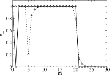
Figure 1: Results for the occupation numbers of single particle states $n_{m}$ in the absence of electron-hole interaction. Circles are HF results and diamonds are exact result (Solid and dotted lines are guides to the eye). Here $\hbar\Omega=3meV$ and $N=20$.

Before we present the numerical results we test the accuracy of our HF approach. In the limit where the electron-hole interaction is absent electrons and holes are independent of each other and exact diagonalization results are known Yang3 . In Fig. 1 we have compared HF occupation numbers of single particle states with those of exact results (In the HF approach occupation numbers are just $n_{m}=v_{m}^{2}$). The following parameters are used: $N=20$, $\hbar\Omega=3meV$, $\mu^{+}=5meV$, and $B=5.9T$. We see that when the effect of quantum fluctuations are included the suppression in the occupation numbers become more broader and less deeper as a function of $m$. Also the positions of the minimum of the density depletion are somewhat different between the two. Nonetheless we see that HF correctly captures qualitatively the right physics of reconstruction near the MDD. The total amount of electron or hole density depletion in the interior of the droplet is exactly one in both cases: $\sum_{m=0}^{15}u_{m}^{2}=1$.

IV.2 Order parameter of reconstructed droplet

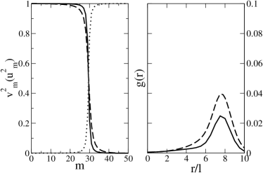
Figure 2: Left panel: Particle occupation numbers $v_{m}^{2}$ (solid line) are plotted as a function of quantum number $m$, which label single particles states. $u_{m}^{2}=1-v_{m}^{2}$ are also plotted (dotted line). Right panel: The order parameter $g(r)$ is plotted as a function of $r$. Here $\hbar\Omega=2.35$meV and $N=30$. For comparison $v_{m}^{2}$ and $g(r)$ for $d=0$ are also shown (dashed lines).

The order parameter, i. e., the condensate density, is

$$g(r) = \langle\Psi_{\uparrow}(r)\Psi_{\downarrow}(r)\rangle$$ (21)

$$= \sum_{mm^{\prime}}\langle c_{m\uparrow}c_{-m^{\prime}\downarrow}\rangle\phi_{m}(r)\phi_{-m^{\prime}}(r),$$

where $\Psi_{\uparrow}(r)=\sum c_{m\uparrow}\phi_{m}(r)$ and $\Psi_{\downarrow}(r)=\sum c_{-m\downarrow}\phi_{-m}(r)$ are electron and hole field operators, respectively. Since the optical selection rule of excitons yang requires $m=m^{\prime}$ we have

$$g(r) = \sum_{m}\langle c_{m\uparrow}c_{-m\downarrow}\rangle|\phi_{m}(r)|^{2}.$$ (22)

Since

$$<c_{m\uparrow}c_{-m\downarrow}>=v_{m}u_{m}=\frac{1}{2}\frac{\Delta_{m}}{E_{m}}.$$ (23)

we have

$$g(r)=\sum_{m}v_{m}u_{m}|\phi_{m}(r)|^{2}.$$ (24)

Note that $|\phi_{m}(r)|^{2}$ is peaked at $r\sim\sqrt{2(m+1)}\ell$ with a width $\ell$ (see Eq.1).

Before we show the results for the order parameter let us first investigate when the MDD is realized. Fig. 2 displays the calculated $v_{m}^{2}$ and $u_{m}^{2}$ for $\hbar\Omega=2.35meV$, $N=30$, $d=0.5\ell$, and $B=5T$. The chemical potential is $\mu^{+}=5.82meV$. The electron and hole occupation numbers, $v_{m}^{2}$, are one except near the edge region $m\approx m_{c}=29$. Note that the radius of the edge of the droplet is $r_{c}=\sqrt{2(m_{c}+1)}\ell$. The electron or hole density of this MDD is given by

$$n_{e,h}(r)=\sum v_{m}^{2}|\phi_{m}(r)|^{2}.$$ (25)

This density looks approximately like a step function

$$n_{e,h}(r)\approx\left\{\begin{array}[]{cl}\frac{1}{2\pi\ell^{2}},&r<\sqrt{2N}\ell\\ 0,&r>\sqrt{2N}\ell.\end{array}\right.$$ (26)

Thus, in a parabolic trap with equal number of electrons and holes a uniform density state can be realized in the strong magnetic field limit with the particle density $1/2\pi\ell^{2}$.

Let us investigate the condensate order parameter for this state. Near the edge, where $m_{c}\sim 29$, both $v_{m}^{2}$ and $u_{m}^{2}$ are non-zero, and, consequently, the order parameter $v_{m}u_{m}$ is non-zero, see Fig. 2. A rough shape of $g(r)$ may be deduced as follows. The product $v_{m}u_{m}$ is roughly given by a delta function $\delta_{m,m_{c}}$. It then follows from Eq. (24) that $g(r)\sim|\phi_{m_{c}}(r)|^{2}$, which is peaked near the edge $r_{c}$. In this MDD electrons and holes are surrounded by condensed excitons near the edge of the dropletpaquet . We have also calculated $v_{m}^{2}$ and $g(r)$ for an increased value for the strength of electron-hole interaction, corresponding to $d=0$ (see dashed lines). We notice that the width of the ring where the order parameter is non-zero becomes larger compared to the case of $d=0.5\ell$, see the dashed curve in the right panel of Fig. 2.

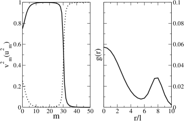
Figure 3: Same as in Fig. 2 but with a smaller value of the strength of the confinement potential $\hbar\Omega=2.27meV$.

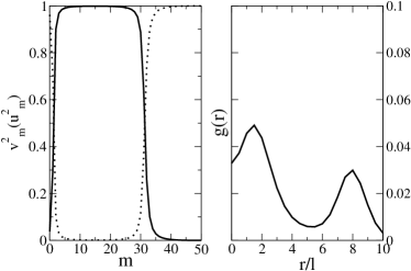
Figure 4: Same as in Fig. 2 but with $\hbar\Omega=2.2meV$.

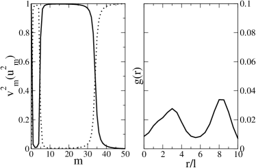
Figure 5: Same as in Fig. 2 but with $\hbar\Omega=2.0meV$.

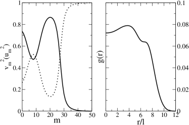
Figure 6: $v_{m}^{2}$ and $g(r)$ for a non-uniform state are shown. The parameters are $\hbar\Omega=2meV$ and $N=20$.

We now show the results on how the uniform MDD reconstructs as the strength of the confinement potential decreases. We will call these reconstructed states nearly uniform droplets. When a smaller value $\hbar\Omega=2.27meV$ is used $v_{m}^{2}$ near $m=0$ deviates from one and $u_{m}^{2}$ starts to take non zero values, see Fig. 3 . The self-consistent value of the chemical potential is $\mu^{+}=5.76$meV. In this case the order parameter develops two peaks. This feature can be understood by investigating the product of $v_{m}u_{m}$: it is non zero near $m=0$ and $m=29$, and two peaks are expected. The quantity $\sum_{m}^{15}u_{m}^{2}=0.92$ gives the number of electrons or holes added from the interior of the droplet to the edge. As $\hbar\Omega$ is reduced further to $2.2meV$ the value of $v_{m}^{2}$ is almost zero at $m=0$ and $\sum_{m}^{15}u_{m}^{2}=1.85$ (see Fig. 4 ). This means that more particles are added from the interior of the droplet to the edge. The value of the chemical potential is $\mu^{+}=5.63$meV. When $\hbar\Omega$ is reduced even further to $2.0meV$ the occupation number $v_{m}^{2}$ is almost zero, not at $m=0$, but, at finite value of $m$ (see Fig. 5 ). In this case the value of the chemical potential is $\mu^{+}=5.35$meV. Note that near $m=3$ the occupation numbers $v_{m}^{2}$ is nearly zero while $u_{m}^{2}$ takes a maximum value. The sum is $\sum_{m}^{15}u_{m}^{2}=4.23$. We conclude from results in Figs. 2 - 5 that with decreasing value of $\hbar\Omega$ the total density added from the interior of the droplet to the edge increases continuously. Similar trend also exists in the case of electron single dots, but there it changes discontinuously and takes integer values. A non-uniform state is also investigated for $\hbar\Omega=2meV$, $\mu^{+}=3.85$meV, and $N=20$. Fig. 6 displays the calculated $v_{m}^{2}$, $u_{m}^{2}$ and the order parameter for this case. The occupation numbers $v_{m}^{2}$ are non-uniform with the average value $1/2$ (For larger values of $\hbar\Omega$ studied above the average occupation number was one). The order parameter is maximum between the center and the edge of the droplet, but does not exhibit a double peak as before. We believe that the results of the HF approach are less reliable in describing non uniform states than nearly uniform states. The results of Fig.6 should thus be taken as rather approximate results.

IV.3 Mean field single particle energies

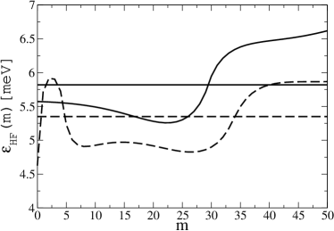
Figure 7: The effective mean field single particle energies as functions of $m$. Solid line is for $\hbar\Omega=2.35meV$ ( see Fig. 1) and the dashed line is for $\hbar\Omega=2.0meV$ ( see Fig. 5). For both cases $N=30$. Horizontal lines represent the values of the chemical potentials.

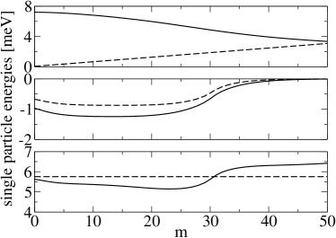
Figure 8: Various terms of the mean field single particle energy for $\hbar\Omega=2.27$meV and $N=30$ are plotted (The corresponding order parameter is plotted in Fig. 3) . Top panel: Solid line represents the intra layer Hartree self energy, $\Sigma_{H,s}(m)$, while dashed line represents the confinement single particle energy. Middle panel: Solid line represents the intra layer exchange self energy, $\Sigma_{X}(m)$, while dashed line represents the inter layer Hartree self energy $\Sigma_{H,d}(m)$. Bottom panel: Solid line represents the effective mean field single particle energy, $\epsilon^{\sigma}_{HF}(m)$, as functions of $m$ while dashed line represents the chemical potential.

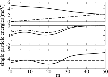
Figure 9: Same as in Fig. 8 but for the non-uniform state. The corresponding order parameter is shown in Fig. 6.

A strong confinement potential pushes particles in each layer to the center of the potential and the particle density of the droplet takes the largest possible value except near the edge of such a MDD. When the confinement potential becomes weaker some particles move from inside of the droplet to the edge, i.e., a reconstruction takes place, and, consequently, the size of the droplet expands in the plane of 2D system. It is not simple to predict exactly where this density depletion takes place in the droplet since it is a consequence of a non-trivial interplay between the confinement potential, Hartree potential, exchange potential, and electron-hole interactions.

The mean field single particle energy $\epsilon^{\sigma}_{HF}(m)$, given in Eq.  (19), reflects this interplay to some degree. A rough shape of $v_{m}^{2}$ may be obtained from the shape of the mean field single particle energy $\epsilon^{\sigma}_{HF}(m)$: In the absence of electron-hole pairing correlation single particle states with $\epsilon^{\sigma}_{HF}(m)$ smaller than the chemical potential are occupied with probability one. However, since we do have pairing in the BEC this is only approximately correct. The mean field single particle energies $\epsilon^{\sigma}_{HF}(m)$ are plotted for $\hbar\Omega=2.35$meV and $2.0$meV in Fig. 7. The corresponding $v_{m}^{2}$ are shown in Fig.2 and Fig.5, respectively. As the strength of the confinement potential decreases the local maximum of $\epsilon^{\sigma}_{HF}(m)$ moves from the center of the droplet and the width of this local maximum becomes broader. The resulting occupation numbers $v_{m}^{2}$ are approximately consistent with the shape of $\epsilon^{\sigma}_{HF}(m)$. Even for a non-uniform droplet the position of the peak in $\epsilon^{\sigma}_{HF}(m)$ coincides with the position of the suppression of $v_{m}^{2}$: see the peak near $m=7$ in $\epsilon^{\sigma}_{HF}(m)$ (Fig.9) and the dip in $v_{m}^{2}$ near $m=7$ (Fig. 6).

The various self energies appearing in $\epsilon^{\sigma}_{HF}(m)$ are plotted for $\hbar\Omega=2.27$meV in Fig. 8. The presence of a peak in $\epsilon^{\sigma}_{HF}(m)$ near $m=0$ is related to the peaks in the self energies $\Sigma_{X}(m)$ and $\Sigma_{H,d}(m)$. The corresponding occupation number $v_{m}^{2}$ decreases near $m=0$ , see Fig. 3. (We notice that $\Sigma_{H,d}(m)$ is almost flat in the region $6<m<20$. $\Sigma_{H,d}(m)$ displays qualitatively the same dependence as the exchange self energy $\Sigma_{X}(m)$. When $d=0$ they are actually identical and are flat for $m<m_{c}$ Yang2 ).

V Conclusions and discussion

We have investigated the shape of the condensed magnetoexcitons in circular traps in strong magnetic fields. Our model consists of a parabolic confinement in lateral directions and a delta function like confinement along the perpendicular axis. We have applied a mean field theory, which is expected to be qualitatively correct. We find that as the strength of the confinement potential weakens, or equivalently as $B$ increases, the uniform state becomes unstable and density depletion starts to occur in the interior of the droplet. We found that the amount of density depletion increases continuously with the decrease in the strength of the confinement potential. As a consequence of these reconstructions the order parameter changes from displaying one peak at the edge to displaying one inner peak and another peak at the edge for decreasing confinement strength. When density depletions are more severe, ie, when the confinement potential is rather weak, the order parameter may display one broad peak.

The reconstruction may be observed experimentally since the spatial shape of the order parameter changes. The structure in the order parameter $g(r)$ may be investigated experimentally by observing angular distribution of photoluminescence since it reflects the Fourier transformed order parameter in the momentum space. An expression for how the PL angular profile depends on the order parameter is given explicitly in Keeling et al Kee . They point out that it may provide a diagnostic for the existence of BEC.

Note that decreasing $\hbar\Omega$ and increasing $B$ has the same effect. Experimentally either of these two parameters may be varied. This can be understood as follows. The strength of the confinement strength enters as a dimensionless parameter in units of the Coulomb energy scale: $\tilde{\gamma}_{\sigma}=\gamma_{\sigma}/(e^{2}/\epsilon\ell)$. The reconstruction of the shape of the droplet will depend on this parameter, which is a function of $B$ and $\hbar\Omega$: $\tilde{\gamma}_{\sigma}\sim(\hbar\Omega)^{2}/B^{3/2}$. It may be easier experimentally to change $B$ than $\hbar\Omega$.

Also it is desirable to increase the particle numbers one order of magnitude and investigate the shape of the condensate droplet. However, this is a non-trivial task since the matrix elements of the particle-particle interactions are difficult to calculate numerically when the quantum number $m$ are large.

We comment on effects that are not investigated in this paper. It would be interesting to study how the corrections to the Hartree Fock theory affect quantitative aspects of the shape of the order parameter. This can be investigated by performing numerical exact diagonalization. Finite quantum well width corrections of the electron and hole wavefunctions will weaken intralayer interactions and hence favor excitonic states over FQHE states. Realistic valence band structure effects yang can be included through the matrix elements of the intra and inter layer Coulomb interaction. Corrections to the lowest Landau level approximation may have quantitative relevance Si .

This work is supported by Korea Research Foundation grant KRF-2003-015-C00223, and by grant No.(R01-1999-00018) from the interdisciplinary research program of the KOSEF.

References

- (1) D. Yoshioka and A.H. MacDonald, J. Phys. Soc. J. 59 4211 (1990).
- (2) Y. Kuramoto and C. Horie, Solid State Commun.25 713 (1978).
- (3) D.Paquet, T.M. Rice, and K. Ueda, Phys. Rev.B, 32 5208 (1985).
- (4) A.V. Korlov and M.A. Liberman, Phys. Rev. B, 50 14077 (1994).
- (5) S.A. Moskalenko, M.A. Liberman, D.W. Snoke, and V.V. Botan, Phys. Rev. B, 66 245316 (2002).
- (6) Y. E. Lozovik and V.I. Yudson, Solid State Commun.19 391 (1976).
- (7) D. Yoshioka and H. Fukuyama, J. Phy. Soc. Jpn. 45 137 (1978).
- (8) Yu. A. Bychkov and E.I. Rashba, Solid State Commun.48 399 (1983).
- (9) L.V. Butov, A. Zrenner, G. Abstreiter, G. Bohm, and G. Weimann, Phys. Rev. Lett. 73, 304 (1994).
- (10) X.M. Chen and J.J. Quinn, Phys. Rev. Lett. 67, 895 (1991).
- (11) O.L. Berman, Y. E. Lozovik, D.W. Snoke, R.D. Coalson, cond-mat/0408581.
- (12) M.N. Anderson, J.R. Ensher, M.R. Matthews, C.E. Wieman, and E.A. Cornell, Science 269 198 (1995).
- (13) V. Negoita and D.W. Snoke, Phys. Rev. B, 60, 2661 (1999).
- (14) L.V. Butov, C.W. Lai, A.L. Ivanov, A.C. Gossard, D.S. Chemla, Na ture 417,47 (2002).
- (15) D. Snoke, S.Denev, Y. Liu, L.Pfeiffer, and K. West, Nature 418,754 (2002).
- (16) X. Zhu, P.B. Littlewood, M.S. Hybertsen, and T.M. Rice, Phys. Rev. Lett. 74, 1633 (1995).
- (17) J. Keeling, L.S. Levitov, and P.B. Littlewood, Phys. Rev. Lett. 92 176402 (2004).
- (18) S.-R. Eric Yang, A. H. MacDonald, and M. D. Johnson, Phys. Rev. Lett. 71, 3194 (1993).
- (19) A. H. MacDonald, S.-R. Eric Yang, and M. D. Johnson, Aust. J. Phys. 46, 345 (1993).
- (20) S.-R. Eric Yang and A. H. MacDonald, Phys. Rev. B 66, 41304(R) (2002).
- (21) R. Ashoori et al., Phys. Rev. Lett68, 3088 (1992); 71, 613 (1993); Naturae (London) 379, 413 (1996).
- (22) T. H. Oosterkamp, J. W. Jassen, L. P. Kouwenhoven, D. G. Austing, T. Honda, and S. Tarucha, Phys. Rev. Lett.82, 2931 (1999).
- (23) O. Klein, C. D. Chamon, D. Tang, D. M. Abuschmagder, U.Meirav, X. G. Wen, M. A. Kanstner, and S. J. Wind, Phys. Rev. Lett.74, 785 (1995).
- (24) S. L. Sondhi, A. Karlhede, and S. A. Kivelson, Phys. Rev. B47,16419 (1993).
- (25) S. M. Reimann, M. Koskinen, M. Manninen, and B. R. Mottelson, Phys. Rev. Lett.83, 3270 (1999).
- (26) C. de. C. Chamon and X. G. Wen, Phys. Rev. B49, 8227 (1994).
- (27) A. Karlhede et al., Phys. Rev. Lett.77 2061 (1996).
- (28) P. M. Petroff, A Lorke, and A. Imamoglu, Physics Today, May 2001.
- (29) S.-R. Eric Yang and L.J. Sham, Phys. Rev. Lett. 58, 2598 (1987).
- (30) S. Siljamki, A. Harju, R. M. Nieminen, V. A. Sverdlov, and P. Hyvnen, Phys. Rev. B 65, 121306 (2002)