Two Superconducting Phases in the $d=3$ Hubbard Model:
Phase Diagram and Specific Heat from Renormalization-Group Calculations

Abstract

The phase diagram of the $d=3$ Hubbard model is calculated as a function of temperature and electron density $\langle n_{i}\rangle$, in the full range of densities between 0 and 2 electrons per site, using renormalization-group theory. An antiferromagnetic phase occurs at lower temperatures, at and near the half-filling density of $\langle n_{i}\rangle=1$. The antiferromagnetic phase is unstable to hole or electron doping of at most 15%, yielding to two distinct ”$\tau$” phases: for large coupling $U/t$, one such phase occurs between 30-35% hole or electron doping, and for small to intermediate coupling $U/t$ another such phase occurs between 10-18% doping. Both $\tau$ phases are distinguished by non-zero hole or electron hopping expectation values at all length scales. Under further doping, the $\tau$ phases yield to hole- or electron-rich disordered phases. We have calculated the specific heat over the entire phase diagram. The low-temperature specific heat of the weak-coupling $\tau$ phase shows a BCS-type exponential decay, indicating a gap in the excitation spectrum, and a cusp singularity at the phase boundary. The strong-coupling $\tau$ phase, on the other hand, has characteristics of BEC-type superconductivity, including a critical exponent $\alpha\approx-1$, and an additional peak in the specific heat above the transition temperature indicating pair formation. In the limit of large Coulomb repulsion, the phase diagram of the $tJ$ model is recovered.

PACS numbers: 74.72.-h, 71.10.Fd, 05.30.Fk, 74.25.Dw

I Introduction

The Hubbard model Hubbard is the simplest realistic (in that it retains particulate dynamics) model of electronic conduction systems. This model should constitute a fair description for many real solid-state physics systems and a starting-point description for those systems with added complexities such as quenched randomness, frustration, and/or spatial anisotropy. The first query that comes to mind, in the study of either experimental or model systems, is on the phase diagram, as a function of physical parameters such as temperature and density. Nevertheless, until recently Hubshort , no estimates, let alone (be it approximate) solutions, were ventured on the phase diagram of the Hubbard model at dimensions greater than $d=1$, at temperatures greater than $T=0$, and densities away from half-filling.

The first approach to a phase diagram problem, in the past before the advent of renormalization-group theory Wilson , had been through a mean-field approximation. However, such method is not useful for the Hubbard model, since, where the characteristic phenomena occur away from half-filling, the off-diagonal term in the Hamiltonian plays a determining role, as we shall see below. There is no ready way to deal with such a dominant quantum mechanical effect using mean-field theory. On the other hand, renormalization-group theory, which some time ago has excelled over mean-field theory in phase diagram studies, is effective. Previous renormalization-group calculations have concentrated on studying the Hubbard model in lower dimensions, at zero temperature, or at half-filling: The zero-temperature (ground-state) properties were successfully obtained in $d=1,2,3$.Hirsch ; FourSpronk In $d=1$ at half-filling, the thermodynamic properties were accurately calculated for finite temperatures.VdzStella In cases where comparison is possible due to the availability of exact results in $d=1$, the renormalization-group results have proven to be very accurate, coming to within about 1% of the exact results.FourSpronk ; VdzStella In $d=2$ at half filling, it was found that no phase transition occurs as a function of temperature.Vdz ; Cannas1 This result was later extended to other fillings in $d=2$ Cannas2 and confirmed by quantum Monte Carlo calculations Cosentini . In $d=3$ at half filling, an antiferromagnetic phase transition as a function of temperature was obtained.Cannas1 One calculation done in $d=3$ at finite temperature and arbitrary chemical potential Cannas2 did not obtain the ”$\tau$” phase reported below and in Ref.Hubshort .

The physics of the Hubbard model in the limit of large Coulomb repulsion is believed to be described by the $tJ$ model Anderson ; BZA . Application of renormalization-group theory to the entire density range of the $tJ$ model at finite temperatures in $d=3$ has yielded FalicovBerker ; FalicovBerkerT , between 30-40% vacancies from $\langle n_{i}\rangle=1$, a novel (dubbed ”$\tau$”) phase in which the electron hopping strength in the Hamiltonian renormalizes to infinity under repeated scale changes, while the system remains partially filled. The calculated topology of the phase diagram, including near the $\tau$ phase a first-order phase transition that is very narrow (less than 2% jump in the electron density) and an antiferromagnetic phase that is unstable to at most 10% vacancies from $\langle n_{i}\rangle=1$, is indeed reminiscent of experimental phase diagram determinations with lanthanide oxides ChouJohn .

While the studies above Hirsch ; FourSpronk ; VdzStella ; Vdz ; Cannas1 ; Cannas2 ; FalicovBerker ; FalicovBerkerT have used position-space renormalization-group approaches, there has recently been a revival of interest in Wilson perturbative renormalization-group methods applied to correlated fermion problems. These methods have long been known to be successful for one-dimensional systems Solyom ; Voit and, in the last few years, for the $d=2$ Hubbard model, they have yielded antiferromagnetic instabilities near half-filling and superconducting instabilities at smaller densities ZanchiSchulzA ; ZanchiSchulzB ; HalbothMetznerA ; HalbothMetznerB ; HonerkampA ; HonerkampB . Because of the perturbative nature of these treatments, their predictions are strictly valid only in the case of weak coupling. The position-space renormalization-group method presented in this paper appears to work over the entire range of coupling strengths, as seen below, and yields definite phase diagrams and thermodynamic functions.

In fact, our approach makes an interesting prediction for the evolution of the Hubbard phase diagram as coupling is increased. We find two distinct $\tau$ phases, one occurring at small to intermediate coupling and the other, inclusive of the $tJ$ model $\tau$ phase, occurring at strong coupling. From an analysis of their specific heat behaviors, we find that the two $\tau$ phases respectively have characteristic properties of a weakly-coupled BCS-type and a strongly-coupled BEC-type superconducting phase. Since high-$T_{c}$ materials share aspects of both limits, and are thought to lie in some intermediate coupling range Junod , our prediction for the Hubbard phase diagram may be directly relevant to the physics of high-$T_{c}$ superconductors.

II The Hubbard Model

The Hubbard model is defined by the Hamiltonian

$$-\beta H= -t\sum_{\langle ij\rangle,\sigma}\left(c_{i\sigma}^{\dagger}c_{j\sigma}+c_{j\sigma}^{\dagger}c_{i\sigma}\right)$$ (1)

$$-U_{0}\sum_{i}n_{i\uparrow}n_{i\downarrow}+\mu_{0}\sum_{i}n_{i}\>,$$

with $\beta=1/kT$, describing electron conduction on a $d$-dimensional hypercubic lattice. Here $c_{i\sigma}^{\dagger}$ and $c_{i\sigma}$ respectively are creation and annihilation operators, obeying anticommutation rules, for an electron with spin $\sigma=\>\uparrow$ or $\downarrow$ at the site $i$ of the lattice; $n_{i\sigma}=c_{i\sigma}^{\dagger}c_{i\sigma}$ and $n_{i}=n_{i\uparrow}+n_{i\downarrow}$ are electron number operators. Each lattice site can accommodate up to two electrons with opposite spins. The index $\langle ij\rangle$ denotes summation over all nearest-neighbor pairs of sites. The three terms of this Hamiltonian respectively incorporate kinetic energy (parametrized by the electron hopping strength $t$), on-site Coulomb repulsion (with coefficient $U_{0}>0$), and chemical potential $\mu_{0}$. It is convenient for our purposes to rearrange Eq.(1) into an equivalent Hamiltonian by grouping into a single lattice summation:

$$-\beta H= \sum_{\langle ij\rangle}\left\{-t\sum_{\sigma}\left(c_{i\sigma}^{\dagger}c_{j\sigma}+c_{j\sigma}^{\dagger}c_{i\sigma}\right)\right.$$ (2)

$$\left.-U\left(n_{i\uparrow}n_{i\downarrow}+n_{j\uparrow}n_{j\downarrow}\right)+\mu\left(n_{i}+n_{j}\right)\right\}$$

$$\equiv \sum_{\langle ij\rangle}\left\{-\beta H(i,j)\right\}\>.$$

The interaction constants are trivially related by $U=U_{0}/2d,\mu=\mu_{0}/2d$, and we have hereby exhibited the individual-pair Hamiltonian $-\beta H(i,j)$.

III Renormalization-Group Transformation

III.1 Exact Formulation in $d=1$

For $d=1$ (with lattice sites $i=1,2,3,\ldots$), the Hubbard Hamiltonian in Eq.(2) takes the form

$$-\beta H=\sum_{i}\left\{-\beta H(i,i+1)\right\},$$ (3)

for which an exact renormalization-group transformation can be formulated. In terms of matrix elements, this exact transformation is FalicovBerker

$$\langle u_{1}u_{3}u_{5}\cdots|e^{-\beta^{\prime}H^{\prime}}|v_{1}v_{3}v_{5}\cdots\rangle=\\ \sum_{w_{2},w_{4},w_{6},\ldots}\langle u_{1}w_{2}u_{3}w_{4}u_{5}w_{6}\cdots|e^{-\beta H}|v_{1}w_{2}v_{3}w_{4}v_{5}w_{6}\cdots\rangle\>,$$ (4)

where $u_{i}$, $v_{i}$, and $w_{i}$ are state variables for lattice site $i$. These variables range over the set $\{\circ,\,\uparrow,\,\downarrow,\,\Updownarrow\}$, by which we represent the no electron, a single electron with spin up, a single electron with spin down, and doubly occupied states. Here and below, the quantities referring to the renormalized (rescaled) system are denoted with a prime. The transformation in Eq.(4) eliminates half of the degrees of freedom in the system, while exactly preserving the partition function ($Z^{\prime}=Z$). However, the transformation cannot be readily implemented, due to the non-commutativity of the operators in the Hamiltonian.

III.2 Approximation in $d=1$

The renormalization-group transformation formulated in Sec.IIIA is implemented approximately, as follows:

$$\begin{split}\mbox{Tr}_{\mbox{\tiny even}}e^{-\beta H}=&\mbox{Tr}_{\mbox{\tiny even}}e^{\sum_{i}\left\{-\beta H(i,i+1)\right\}}\\ =&\mbox{Tr}_{\mbox{\tiny even}}e^{\sum_{i}^{\mbox{\tiny even}}\left\{-\beta H(i-1,i)-\beta H(i,i+1)\right\}}\\ \simeq&\prod_{i}^{\mbox{\tiny even}}\mbox{Tr}_{i}e^{\left\{-\beta H(i-1,i)-\beta H(i,i+1)\right\}}\\ =&\prod_{i}^{\mbox{\tiny even}}e^{-\beta^{\prime}H^{\prime}(i-1,i+1)}\\ \simeq&e^{\sum_{i}^{\mbox{\tiny even}}\left\{-\beta^{\prime}H^{\prime}(i-1,i+1)\right\}}=e^{-\beta^{\prime}H^{\prime}}.\end{split}$$ (5)

In the two approximate steps, marked by $\simeq$ in Eq.(5), we ignore the non-commutation of operators separated beyond three consecutive sites of the unrenormalized system. Since each of these two steps involves the same approximation but in opposite directions, some mutual compensation can be expected. The success of this approximation at predicting finite-temperature behavior has been verified in earlier studies of quantum spin systems SuzTak ; TakSuz .

The algebraic content of the renormalization-group mapping can be extracted from Eq.(5) as

$$e^{-\beta^{\prime}H^{\prime}(i,k)}=\mbox{Tr}_{j}e^{-\beta H(i,j)-\beta H(j,k)},$$ (6)

where $i,j,k$ are three consecutive sites of the unrenormalized system. The operators $-\beta^{\prime}H^{\prime}(i,k)$ and $-\beta H(i,j)-\beta H(j,k)$ act on the space of two-site and three-site states respectively, so that, in terms of matrix elements,

$$\langle u_{i}v_{k}|e^{-\beta^{\prime}H^{\prime}(i,k)}|\bar{u}_{i}\bar{v}_{k}\rangle=\\ \sum_{w_{j}}\langle u_{i}\,w_{j}\,v_{k}|e^{-\beta H(i,j)-\beta H(j,k)}|\bar{u}_{i}\,w_{j}\,\bar{v}_{k}\rangle\>,$$ (7)

where $u_{i},w_{j},v_{k},\bar{u}_{i},\bar{v}_{k}$ are single-site state variables. Eq.(7) indicates the contraction of a $64\times 64$ matrix on the right into a $16\times 16$ matrix on the left. This is greatly simplified by the use of two- and three-site basis states that block-diagonalize respectively the left and right sides of Eq.(7). These basis states are the eigenstates of total particle number, total spin magnitude, total spin $z$-component, and parity. We denote the set of 16 two-site eigenstates by $\{|\phi_{p}\rangle\}$ and the set of 64 three-site eigenstates by $\{|\psi_{q}\rangle\}$, and list them in Tables I and II.   Eq.(7) is rewritten as

$$\langle\phi_{p}|e^{-\beta^{\prime}H^{\prime}(i,k)}|\phi_{\bar{p}}\rangle=\\ \sum_{\begin{subarray}{c}u,v,\bar{u},\\ \bar{v},w\end{subarray}}\sum_{\begin{subarray}{c}q,\bar{q}\end{subarray}}\langle\phi_{p}|u_{i}v_{k}\rangle\langle u_{i}w_{j}v_{k}|\psi_{q}\rangle\langle\psi_{q}|e^{-\beta H(i,j)-\beta H(j,k)}|\psi_{\bar{q}}\rangle\cdot\\ \langle\psi_{\bar{q}}|\bar{u}_{i}w_{j}\bar{v}_{k}\rangle\langle\bar{u}_{i}\bar{v}_{k}|\phi_{\bar{p}}\rangle\>.$$ (8)

In the above equation, with the eigenstates shown in Tables I and II, the largest block in $\langle\phi_{p}|e^{-\beta^{\prime}H^{\prime}(i,k)}|\phi_{\bar{p}}\rangle$ is $2\times 2$ and the largest block in $\langle\psi_{q}|e^{-\beta H(i,j)-\beta H(j,k)}|\psi_{\bar{q}}\rangle$ is $4\times 4$. (In previous work Hubshort , some matrix elements in these blocks were incorrectly derived). Eq.(8) yields eleven independent elements for the matrix $\langle\phi_{p}|e^{-\beta^{\prime}H^{\prime}(i,k)}|\phi_{\bar{p}}\rangle$ of the renormalized system. These we label $\gamma_{p}$, as shown in Appendix A. The values of the $\gamma_{p}$ in terms of the matrix elements of the unrenormalized system, dictated by the right-hand side of Eq.(8), are also given in Appendix A.

$n$	$p$	$s$	$m_{s}$	Two-site basis states
$0$	$+$	$0$	$0$	$|\phi_{1}\rangle=|\circ\circ\rangle$
$1$	$+$	$1/2$	$1/2$	$|\phi_{2}\rangle=\frac{1}{\sqrt{2}}\{|\uparrow\circ\rangle+|\circ\uparrow\rangle\}$
$1$	$-$	$1/2$	$1/2$	$|\phi_{4}\rangle=\frac{1}{\sqrt{2}}\{|\uparrow\circ\rangle-|\circ\uparrow\rangle\}$
$2$	$+$	$0$	$0$	$|\phi_{6}\rangle=\frac{1}{\sqrt{2}}\{|\Updownarrow\circ\rangle+|\circ\Updownarrow\rangle\}$
$2$	$-$	$0$	$0$	$|\phi_{7}\rangle=\frac{1}{\sqrt{2}}\{|\Updownarrow\circ\rangle-|\circ\Updownarrow\rangle\},$
				$|\phi_{8}\rangle=\frac{1}{\sqrt{2}}\{|\uparrow\downarrow\rangle-|\downarrow\uparrow\rangle\}$
$2$	$+$	$1$	$1$	$|\phi_{9}\rangle=|\uparrow\uparrow\rangle$
$2$	$+$	$1$	$0$	$|\phi_{10}\rangle=\frac{1}{\sqrt{2}}\{|\uparrow\downarrow\rangle+|\downarrow\uparrow\rangle\}$
$3$	$+$	$1/2$	$1/2$	$|\phi_{12}\rangle=\frac{1}{\sqrt{2}}\{|\Updownarrow\uparrow\rangle+|\uparrow\Updownarrow\rangle\}$
$3$	$-$	$1/2$	$1/2$	$|\phi_{14}\rangle=\frac{1}{\sqrt{2}}\{|\Updownarrow\uparrow\rangle-|\uparrow\Updownarrow\rangle\}$
$4$	$+$	$0$	$0$	$|\phi_{16}\rangle=|\Updownarrow\Updownarrow\rangle$

Table I: The two-site basis states used in the derivation of the recursion relations, in Eq. (8). In these basis states, $e^{-\beta^{\prime}H^{\prime}(i,k)}$ is diagonal, with the exception of a $2\times 2$ block involving $|\phi_{6}\rangle$ and $|\phi_{8}\rangle$. The corresponding particle number ($n$), parity ($p$), total spin ($s$), and total spin $z$-component ($m_{s}$) quantum numbers are also given. The states $|\phi_{3}\rangle$, $|\phi_{5}\rangle$, $|\phi_{11}\rangle$, $|\phi_{13}\rangle$, $|\phi_{15}\rangle$ are obtained by spin reversal from $|\phi_{2}\rangle$, $|\phi_{4}\rangle$, $|\phi_{9}\rangle$, $|\phi_{12}\rangle$, $|\phi_{14}\rangle$, respectively.

$n$	$p$	$s$	$m_{s}$	Three-site basis states
$0$	$+$	$0$	$0$	$|\psi_{1}\rangle=|\circ\circ\,\circ\rangle$
$1$	$+$	$1/2$	$1/2$	$|\psi_{2}\rangle=|\circ\uparrow\circ\rangle,\>|\psi_{3}\rangle=\frac{1}{\sqrt{2}}\{|\uparrow\circ\,\circ\rangle+|\circ\,\circ\uparrow\rangle\}$
$1$	$-$	$1/2$	$1/2$	$|\psi_{6}\rangle=\frac{1}{\sqrt{2}}\{|\uparrow\circ\,\circ\rangle-|\circ\,\circ\uparrow\rangle\}$
$2$	$+$	$0$	$0$	$|\psi_{8}\rangle=\frac{1}{2}\{|\uparrow\downarrow\circ\rangle-|\downarrow\uparrow\circ\rangle-|\circ\uparrow\downarrow\rangle+|\circ\downarrow\uparrow\rangle\},$
				$|\psi_{9}\rangle=|\circ\Updownarrow\circ\rangle,\>|\psi_{10}\rangle=\frac{1}{\sqrt{2}}\{|\Updownarrow\circ\,\circ\rangle+|\circ\,\circ\Updownarrow\rangle\}$
$2$	$-$	$0$	$0$	$|\psi_{11}\rangle=\frac{1}{2}\{|\uparrow\downarrow\circ\rangle-|\downarrow\uparrow\circ\rangle+|\circ\uparrow\downarrow\rangle-|\circ\downarrow\uparrow\rangle\},$
				$|\psi_{12}\rangle=\frac{1}{\sqrt{2}}\{|\uparrow\circ\downarrow\rangle-|\downarrow\circ\uparrow\rangle\},$
				$|\psi_{13}\rangle=\frac{1}{\sqrt{2}}\{|\Updownarrow\circ\,\circ\rangle-|\circ\,\circ\Updownarrow\rangle\}$
$2$	$+$	$1$	$1$	$|\psi_{14}\rangle=|\uparrow\circ\uparrow\rangle,\>|\psi_{15}\rangle=\frac{1}{\sqrt{2}}\{|\uparrow\uparrow\circ\rangle+|\circ\uparrow\uparrow\rangle\}$
$2$	$+$	$1$	$0$	$|\psi_{16}\rangle=\frac{1}{2}\{|\uparrow\downarrow\circ\rangle+|\downarrow\uparrow\circ\rangle+|\circ\uparrow\downarrow\rangle+|\circ\downarrow\uparrow\rangle\},$
				$|\psi_{17}\rangle=\frac{1}{\sqrt{2}}\{|\uparrow\circ\downarrow\rangle+|\downarrow\circ\uparrow\rangle\}$
$2$	$-$	$1$	$1$	$|\psi_{20}\rangle=\frac{1}{\sqrt{2}}\{|\uparrow\uparrow\circ\rangle-|\circ\uparrow\uparrow\rangle\}$
$2$	$-$	$1$	$0$	$|\psi_{21}\rangle=\frac{1}{2}\{|\uparrow\downarrow\circ\rangle+|\downarrow\uparrow\circ\rangle-|\circ\uparrow\downarrow\rangle-|\circ\downarrow\uparrow\rangle\}$
$3$	$+$	$1/2$	$1/2$	$|\psi_{23}\rangle=\frac{1}{\sqrt{6}}\{2|\uparrow\downarrow\uparrow\rangle-|\uparrow\uparrow\downarrow\rangle-|\downarrow\uparrow\uparrow\rangle\},$
				$|\psi_{24}\rangle=\frac{1}{\sqrt{2}}\{|\uparrow\Updownarrow\circ\rangle+|\circ\Updownarrow\uparrow\rangle\},$
				$|\psi_{25}\rangle=\frac{1}{\sqrt{2}}\{|\uparrow\circ\Updownarrow\rangle+|\Updownarrow\circ\uparrow\rangle\},$
				$|\psi_{26}\rangle=\frac{1}{\sqrt{2}}\{|\Updownarrow\uparrow\circ\rangle+|\circ\uparrow\Updownarrow\rangle\}$
$3$	$-$	$1/2$	$1/2$	$|\psi_{31}\rangle=\frac{1}{\sqrt{2}}\{|\uparrow\uparrow\downarrow\rangle-|\downarrow\uparrow\uparrow\rangle\},$
				$|\psi_{32}\rangle=\frac{1}{\sqrt{2}}\{|\uparrow\Updownarrow\circ\rangle-|\circ\Updownarrow\uparrow\rangle\},$
				$|\psi_{33}\rangle=\frac{1}{\sqrt{2}}\{|\uparrow\circ\Updownarrow\rangle-|\Updownarrow\circ\uparrow\rangle\},$
				$|\psi_{34}\rangle=\frac{1}{\sqrt{2}}\{|\Updownarrow\uparrow\circ\rangle-|\circ\uparrow\Updownarrow\rangle\}$
$3$	$+$	$3/2$	$3/2$	$|\psi_{39}\rangle=|\uparrow\uparrow\uparrow\rangle$
$3$	$+$	$3/2$	$1/2$	$|\psi_{40}\rangle=\frac{1}{\sqrt{3}}\{|\uparrow\downarrow\uparrow\rangle+|\uparrow\uparrow\downarrow\rangle+|\downarrow\uparrow\uparrow\rangle\}$
$4$	$+$	$0$	$0$	$|\psi_{43}\rangle=|\Updownarrow\circ\Updownarrow\rangle,\>|\psi_{44}\rangle=\frac{1}{\sqrt{2}}\{|\Updownarrow\Updownarrow\circ\rangle+|\circ\Updownarrow\Updownarrow\rangle\},$
				$|\psi_{45}\rangle=\frac{1}{2}\{|\uparrow\downarrow\Updownarrow\rangle-|\downarrow\uparrow\Updownarrow\rangle-|\Updownarrow\uparrow\downarrow\rangle+|\Updownarrow\downarrow\uparrow\rangle\}$
$4$	$-$	$0$	$0$	$|\psi_{46}\rangle=\frac{1}{2}\{|\downarrow\uparrow\Updownarrow\rangle-|\uparrow\downarrow\Updownarrow\rangle-|\Updownarrow\uparrow\downarrow\rangle+|\Updownarrow\downarrow\uparrow\rangle\},$
				$|\psi_{47}\rangle=\frac{1}{\sqrt{2}}\{|\uparrow\Updownarrow\downarrow\rangle-|\downarrow\Updownarrow\uparrow\rangle\},$
				$|\psi_{48}\rangle=\frac{1}{\sqrt{2}}\{|\Updownarrow\Updownarrow\circ\rangle-|\circ\Updownarrow\Updownarrow\rangle\}$
$4$	$+$	$1$	$1$	$|\psi_{49}\rangle=|\uparrow\Updownarrow\uparrow\rangle,\>|\psi_{50}\rangle=\frac{1}{\sqrt{2}}\{|\uparrow\uparrow\Updownarrow\rangle+|\Updownarrow\uparrow\uparrow\rangle\}$
$4$	$+$	$1$	$0$	$|\psi_{51}\rangle=\frac{1}{2}\{|\uparrow\downarrow\Updownarrow\rangle+|\downarrow\uparrow\Updownarrow\rangle+|\Updownarrow\uparrow\downarrow\rangle+|\Updownarrow\downarrow\uparrow\rangle\},$
				$|\psi_{52}\rangle=\frac{1}{\sqrt{2}}\{|\uparrow\Updownarrow\downarrow\rangle+|\downarrow\Updownarrow\uparrow\rangle\}$
$4$	$-$	$1$	$1$	$|\psi_{55}\rangle=\frac{1}{\sqrt{2}}\{|\uparrow\uparrow\Updownarrow\rangle-|\Updownarrow\uparrow\uparrow\rangle\}$
$4$	$-$	$1$	$0$	$|\psi_{56}\rangle=\frac{1}{2}\{|\uparrow\downarrow\Updownarrow\rangle+|\downarrow\uparrow\Updownarrow\rangle-|\Updownarrow\uparrow\downarrow\rangle-|\Updownarrow\downarrow\uparrow\rangle\}$
$5$	$+$	$1/2$	$1/2$	$|\psi_{58}\rangle=|\Updownarrow\uparrow\Updownarrow\rangle,\>|\psi_{59}\rangle=\frac{1}{\sqrt{2}}\{|\uparrow\Updownarrow\Updownarrow\rangle+|\Updownarrow\Updownarrow\uparrow\rangle\}$
$5$	$-$	$1/2$	$1/2$	$|\psi_{62}\rangle=\frac{1}{\sqrt{2}}\{|\Updownarrow\Updownarrow\uparrow\rangle-|\uparrow\Updownarrow\Updownarrow\rangle\}$
$6$	$+$	$0$	$0$	$|\psi_{64}\rangle=|\Updownarrow\Updownarrow\Updownarrow\rangle$

Table II: The three-site basis states used in the derivation of the recursion relations, in Eq. (8). In these basis states, $e^{-\beta H(i,j)-\beta H(j,k)}$ is block-diagonal, with the largest blocks being $4\times 4$ (see Table IV). The corresponding particle number ($n$), parity ($p$), total spin ($s$), and total spin $z$-component ($m_{s}$) quantum numbers are also given. The states $|\phi_{4-5}\rangle$, $|\phi_{7}\rangle$, $|\phi_{18-19}\rangle$, $|\phi_{22}\rangle$, $|\phi_{27-30}\rangle$, $|\phi_{35-38}\rangle$, $|\phi_{41-42}\rangle$, $|\phi_{53-54}\rangle$, $|\phi_{57}\rangle$, $|\phi_{60-61}\rangle$, $|\phi_{63}\rangle$ are obtained by spin reversal from $|\phi_{2-3}\rangle$, $|\phi_{6}\rangle$, $|\phi_{14-15}\rangle$, $|\phi_{20}\rangle$, $|\phi_{23-26}\rangle$, $|\phi_{31-34}\rangle$, $|\phi_{39-40}\rangle$, $|\phi_{49-50}\rangle$, $|\phi_{55}\rangle$, $|\phi_{58-59}\rangle$, $|\phi_{62}\rangle$, respectively.

III.3 Hamiltonian Closed Form under
the Renormalization-Group Transformation

Since eleven interaction strengths can be independently fixed by the eleven $\gamma_{p}$, the Hamiltonian $-\beta^{\prime}H^{\prime}$ which is embodied in Appendix A has a more general form than that of the Hubbard Hamiltonian in Eq.(2). This generalized form of the pair Hamiltonian is

$$\begin{split}-&\beta H(i,j)=\\ &-\sum_{\begin{subarray}{c}\sigma\end{subarray}}\>\left[\,t_{0}\,h_{i\,-\sigma}h_{j\,-\sigma}+t_{1}(h_{i\,-\sigma}n_{j\,-\sigma}+n_{i\,-\sigma}h_{j\,-\sigma})\right.\\ &\left.+t_{2}\,n_{i\,-\sigma}n_{j\,-\sigma}\right]\left(c^{\dagger}_{i\sigma}c_{j\sigma}+c^{\dagger}_{j\sigma}c_{i\sigma}\right)\\ &-t_{x}\left(c^{\dagger}_{i\uparrow}c_{j\uparrow}c^{\dagger}_{i\downarrow}c_{j\downarrow}+c^{\dagger}_{j\uparrow}c_{i\uparrow}c^{\dagger}_{j\downarrow}c_{i\downarrow}\right)\\ &-U\left(n_{i\uparrow}n_{i\downarrow}+n_{j\uparrow}n_{j\downarrow}\right)+\mu\left(n_{i}+n_{j}\right)+J\,\vec{S}_{i}\cdot\vec{S}_{j}\\ &+V_{2}n_{i}n_{j}+V_{3}\left(n_{i\uparrow}n_{i\downarrow}n_{j}+n_{i}n_{j\uparrow}n_{j\downarrow}\right)\\ &+V_{4}n_{i\uparrow}n_{i\downarrow}n_{j\uparrow}n_{j\downarrow}\>+\>G\>,\end{split}$$ (9)

where $h_{i\sigma}\equiv 1-n_{i\sigma}$ is the hole (vacancy) operator and $\vec{S}_{i}=\sum_{\sigma,\bar{\sigma}}c^{\dagger}_{i\sigma}\vec{s}_{\sigma\bar{\sigma}}c_{i\bar{\sigma}}$, with $\vec{s}_{\sigma\bar{\sigma}}$ the vector of Pauli spin matrices, is the spin operator at site i. In general, the Hubbard Hamiltonian, after one renormalization-group transformation, maps onto this generalized Hamiltonian, which has a form that stays closed under further renormalization-group transformations.

The kinetic energy part of the Hamiltonian in Eq.(9) distinguishes the four types of nearest-neighbor hopping events: i) vacancy hopping (the $t_{0}$ term): a vacancy (hole) hopping against a background of single-electron occupancy (half-filling); ii) pair breaking or pair making (the $t_{1}$ term): doubly occupied and completely unoccupied nearest-neighbor sites reverting to half-filling, or the reverse process; iii) pair hopping (the $t_{2}$ term): a pair hopping against a background of half-filling; iv) vacancy - pair interchange (the $t_{x}$ term): doubly occupied and completely unoccupied nearest-neighbor sites exchanging positions.

The generalized Hamiltonian of Eq.(9) reduces to the Hubbard Hamiltonian of Eq.(2) for $t_{0}=t_{1}=t_{2}=t$ and $t_{x}=J=V_{2}=V_{3}=V_{4}=G=0\>.$ The renormalization-group flows occur in the 10-dimensional interaction space of the generalized Hamiltonian; the 3-dimensional interaction space of the Hubbard Hamiltonian contains the initial conditions of the renormalization-group flows.

The matrix elements of the renormalized pair Hamiltonian $-\beta^{\prime}H^{\prime}(i,k)$ are given in Table III in terms of the renormalized interaction constants. Table III allows us to solve for the renormalized interaction constants in terms of the $\gamma_{p}$ given in Appendix A:

$$t_{0}^{\prime}=\frac{1}{2}\ln\frac{\gamma_{4}}{\gamma_{2}},\qquad t_{1}^{\prime}=u\frac{\gamma_{0}}{\gamma_{8}-\gamma_{6}},$$

$$t_{2}^{\prime}=\frac{1}{2}\ln\frac{\gamma_{12}}{\gamma_{14}},\qquad t_{x}^{\prime}=\frac{1}{2}\left(u-v+\ln\gamma_{7}\right),$$

$$U^{\prime}=\frac{1}{2}\left(u-v+\ln\frac{\gamma_{2}^{2}\gamma_{4}^{2}}{\gamma_{1}^{2}\gamma_{7}}\right),\qquad\mu^{\prime}=\frac{1}{2}\ln\frac{\gamma_{2}\gamma_{4}}{\gamma_{1}^{2}},$$

$$J^{\prime}=-u-v+\ln\gamma_{9},\qquad V_{2}^{\prime}=\frac{1}{4}\ln\frac{\gamma_{1}^{4}\gamma_{9}^{3}}{\gamma_{2}^{4}\gamma_{4}^{4}}+\frac{1}{4}(u+v),$$

$$V_{3}^{\prime}=\frac{1}{2}\ln\frac{\gamma_{2}^{3}\gamma_{4}^{3}\gamma_{12}\gamma_{14}}{\gamma_{1}^{2}\gamma_{7}\gamma_{9}^{3}}-v,\qquad V_{4}^{\prime}=\ln\frac{\gamma_{1}\gamma_{7}\gamma_{9}^{3}\gamma_{16}}{\gamma_{2}^{2}\gamma_{4}^{2}\gamma_{12}^{2}\gamma_{14}^{2}}+2v,$$

$$G^{\prime}=\ln\gamma_{1},$$ (10)

where

$$v=\frac{1}{2}\ln\left(\gamma_{6}\gamma_{8}-\gamma_{0}^{2}\right),$$

$$u=\frac{\gamma_{8}-\gamma_{6}}{\sqrt{\left(\gamma_{8}-\gamma_{6}\right)^{2}+4\gamma_{0}^{2}}}\cosh^{-1}\left(\frac{\gamma_{8}+\gamma_{6}}{2e^{v}}\right).$$

$$\begin{array}[]{|c||c|c|c|c|c|c|}\hline\cr-\beta^{\prime}H^{\prime}(i,k)&\phi_{1}&\phi_{2}&\phi_{4}&\phi_{7}&\phi_{9}&\phi_{10}\\ \hline\cr\phi_{1}&G^{\prime}&\lx@intercol\hfil\hfil\lx@intercol\vrule\lx@intercol\\ \cline{1-3}\cr\phi_{2}&&\parbox{25.29494pt}{\centering$-t_{0}^{\prime}+\mu^{\prime}+G^{\prime}$\@add@centering}&\lx@intercol\hfil 0\hfil\lx@intercol\vrule\lx@intercol\\ \cline{1-1}\cr\cline{3-4}\cr\phi_{4}&\lx@intercol\hfil\hfil\lx@intercol\vrule\lx@intercol&\parbox{25.29494pt}{\centering$t_{0}^{\prime}+\mu^{\prime}+G^{\prime}$\@add@centering}&\lx@intercol\hfil\hfil\lx@intercol\vrule\lx@intercol\\ \cline{1-1}\cr\cline{4-5}\cr\phi_{7}&\lx@intercol\hfil\hfil\lx@intercol\vrule\lx@intercol&\lx@intercol\hfil\parbox{28.90755pt}{\centering$t_{x}^{\prime}-U^{\prime}+2\mu^{\prime}+G^{\prime}$\@add@centering}\hfil\lx@intercol\vrule\lx@intercol&\lx@intercol\hfil\hfil\lx@intercol\vrule\lx@intercol\\ \cline{1-1}\cr\cline{5-6}\cr\phi_{9}&\lx@intercol\hfil 0\hfil\lx@intercol\vrule\lx@intercol&\lx@intercol\hfil\parbox{28.90755pt}{\centering$2\mu^{\prime}+\frac{1}{4}J^{\prime}+V_{2}^{\prime}+G^{\prime}$\@add@centering}\hfil\lx@intercol\vrule\lx@intercol&\\ \cline{1-1}\cr\cline{6-7}\cr\phi_{10}&\lx@intercol\hfil\hfil\lx@intercol\vrule\lx@intercol&\parbox{28.90755pt}{\centering$2\mu^{\prime}+\frac{1}{4}J^{\prime}+V_{2}^{\prime}+G^{\prime}$\@add@centering}\\ \hline\cr\end{array}$$

$$\begin{array}[]{|c||c|c|}\hline\cr-\beta^{\prime}H^{\prime}(i,k)&\phi_{6}&\phi_{8}\\ \hline\cr\phi_{6}&-t_{x}^{\prime}-U^{\prime}+2\mu^{\prime}+G^{\prime}&2t_{1}^{\prime}\\ \cline{1-3}\cr\phi_{8}&2t_{1}^{\prime}&2\mu^{\prime}-\frac{3}{4}J^{\prime}+V_{2}^{\prime}+G^{\prime}\\ \hline\cr\end{array}$$

$$\begin{array}[]{|c||c|c|c|}\hline\cr-\beta^{\prime}H^{\prime}(i,k)&\phi_{12}&\phi_{14}&\phi_{16}\\ \hline\cr\phi_{12}&\parbox{54.2025pt}{\centering$t_{2}^{\prime}-U^{\prime}+3\mu^{\prime}$\\ $+2V_{2}^{\prime}+V_{3}^{\prime}+G^{\prime}$\@add@centering}&\lx@intercol\hfil\lx@intercol\vrule\lx@intercol\\ \cline{1-3}\cr\phi_{14}&\lx@intercol\hfil\hfil\lx@intercol\vrule\lx@intercol&\parbox{54.2025pt}{\centering$-t_{2}^{\prime}-U^{\prime}+3\mu^{\prime}$\\ $+2V_{2}^{\prime}+V_{3}^{\prime}+G^{\prime}$\@add@centering}&0\\ \cline{1-1}\cr\cline{3-4}\cr\phi_{16}&\lx@intercol\hfil 0\hfil\lx@intercol\vrule\lx@intercol&\parbox{57.81621pt}{\centering$-2U^{\prime}+4\mu^{\prime}+4V_{2}^{\prime}$\\ $+4V_{3}^{\prime}+V_{4}^{\prime}+G^{\prime}$\@add@centering}\\ \hline\cr\end{array}$$

Table III: Block-diagonal matrix of the renormalized two-site Hamiltonian $-\beta^{\prime}H^{\prime}(i,k)$. The Hamiltonian being invariant under spin-reversal, the spin-flipped matrix elements are not shown.

$$\begin{array}[]{|c||c|}\hline\cr&\psi_{1}\\ \hline\cr\psi_{1}&0\\ \hline\cr\end{array}\quad\begin{array}[]{|c||c|c|}\hline\cr&\psi_{2}&\psi_{3}\\ \hline\cr\psi_{2}&2\mu&-\sqrt{2}t_{0}\\ \hline\cr\psi_{3}&-\sqrt{2}t_{0}&\mu\\ \hline\cr\end{array}\quad\begin{array}[]{|c||c|}\hline\cr&\psi_{6}\\ \hline\cr\psi_{6}&\mu\\ \hline\cr\end{array}$$

$$\begin{array}[]{|c||c|c|c|c|}\hline\cr&\psi_{9}&\psi_{10}&\psi_{11}&\psi_{12}\\ \hline\cr\psi_{9}&-2U+4\mu&-\sqrt{2}t_{x}&2t_{1}&0\\ \hline\cr\psi_{10}&-\sqrt{2}t_{x}&-U+2\mu&\sqrt{2}t_{1}&0\\ \hline\cr\psi_{11}&2t_{1}&\sqrt{2}t_{1}&3\mu-\frac{3}{4}J+V_{2}&-\sqrt{2}t_{0}\\ \hline\cr\psi_{12}&0&0&-\sqrt{2}t_{0}&2\mu\\ \hline\cr\end{array}$$

$$\begin{array}[]{|c||c|c|}\hline\cr&\psi_{8}&\psi_{13}\\ \hline\cr\psi_{8}&3\mu-\frac{3}{4}J+V_{2}&\sqrt{2}t_{1}\\ \hline\cr\psi_{13}&\sqrt{2}t_{1}&-U+2\mu\\ \hline\cr\end{array}\quad\begin{array}[]{|c||c|c|}\hline\cr&\psi_{14}&\psi_{15}\\ \hline\cr\psi_{14}&2\mu&-\sqrt{2}t_{0}\\ \hline\cr\psi_{15}&-\sqrt{2}t_{0}&3\mu+\frac{1}{4}J+V_{2}\\ \hline\cr\end{array}$$

$$\begin{array}[]{|c||c|c|}\hline\cr&\psi_{16}&\psi_{17}\\ \hline\cr\psi_{16}&3\mu+\frac{1}{4}J+V_{2}&-\sqrt{2}t_{0}\\ \hline\cr\psi_{17}&-\sqrt{2}t_{0}&2\mu\\ \hline\cr\end{array}\quad\begin{array}[]{|c||c|}\hline\cr&\psi_{20}\\ \hline\cr\psi_{20}&\parbox{28.90755pt}{\centering$3\mu+\frac{1}{4}J+V_{2}$\@add@centering}\\ \hline\cr\end{array}\quad\begin{array}[]{|c||c|}\hline\cr&\psi_{21}\\ \hline\cr\psi_{21}&\parbox{28.90755pt}{\centering$3\mu+\frac{1}{4}J+V_{2}$\@add@centering}\\ \hline\cr\end{array}$$

$$\begin{array}[]{|c||c|c|c|c|c|}\hline\cr&\psi_{24}&\psi_{25}&\psi_{26}&\psi_{31}\\ \hline\cr\psi_{24}&\parbox{43.36243pt}{\centering$-2U+5\mu+2V_{2}+V_{3}$\@add@centering}&-t_{x}&t_{2}&t_{1}\\ \hline\cr\psi_{25}&-t_{x}&-U+3\mu&-t_{0}&t_{1}\\ \hline\cr\psi_{26}&t_{2}&-t_{0}&\parbox{36.135pt}{\centering$-U+4\mu+2V_{2}+V_{3}$\@add@centering}&0\\ \hline\cr\psi_{31}&t_{1}&t_{1}&0&\parbox{36.135pt}{\centering$4\mu+2V_{2}$\@add@centering}\\ \hline\cr\end{array}$$

$$\begin{array}[]{|c||c|c|c|c|}\hline\cr&\psi_{23}&\psi_{32}&\psi_{33}&\psi_{34}\\ \hline\cr\psi_{23}&4\mu-J+2V_{2}&-\sqrt{3}t_{1}&-\sqrt{3}t_{1}&0\\ \hline\cr\psi_{32}&-\sqrt{3}t_{1}&\parbox{43.36243pt}{\centering$-2U+5\mu+2V_{2}+V_{3}$\@add@centering}&-t_{x}&t_{2}\\ \hline\cr\psi_{33}&-\sqrt{3}t_{1}&-t_{x}&-U+3\mu&t_{0}\\ \hline\cr\psi_{34}&0&t_{2}&t_{0}&\parbox{43.36243pt}{\centering$-U+4\mu+2V_{2}+V_{3}$\@add@centering}\\ \hline\cr\end{array}$$

$$\begin{array}[]{|c||c|}\hline\cr&\psi_{39}\\ \hline\cr\psi_{39}&4\mu+\frac{1}{2}J+2V_{2}\\ \hline\cr\end{array}\quad\begin{array}[]{|c||c|}\hline\cr&\psi_{40}\\ \hline\cr\psi_{40}&4\mu+\frac{1}{2}J+2V_{2}\\ \hline\cr\end{array}$$

$$\begin{array}[]{|c||c|c|c|c|}\hline\cr&\psi_{43}&\psi_{44}&\psi_{46}&\psi_{47}\\ \hline\cr\psi_{43}&-2U+4\mu&-\sqrt{2}t_{x}&-2t_{1}&0\\ \hline\cr\psi_{44}&-\sqrt{2}t_{x}&\parbox{50.58878pt}{\centering$-3U+6\mu+4V_{2}+4V_{3}+V_{4}$\@add@centering}&-\sqrt{2}t_{1}&0\\ \hline\cr\psi_{46}&-2t_{1}&-\sqrt{2}t_{1}&\parbox{50.58878pt}{\centering$-U+5\mu-\frac{3}{4}J+3V_{2}+V_{3}$\@add@centering}&-\sqrt{2}t_{2}\\ \hline\cr\psi_{47}&0&0&-\sqrt{2}t_{2}&\parbox{43.36243pt}{\centering$-2U+6\mu+4V_{2}+2V_{3}$\@add@centering}\\ \hline\cr\end{array}$$

$$\begin{array}[]{|c||c|c|}\hline\cr&\psi_{45}&\psi_{48}\\ \hline\cr\psi_{45}&-U+5\mu-\frac{3}{4}J+3V_{2}+V_{3}&-\sqrt{2}t_{1}\\ \hline\cr\psi_{48}&-\sqrt{2}t_{1}&-3U+6\mu+4V_{2}+4V_{3}+V_{4}\\ \hline\cr\end{array}$$

$$\begin{array}[]{|c||c|c|}\hline\cr&\psi_{49}&\psi_{50}\\ \hline\cr\psi_{49}&-2U+6\mu+4V_{2}+2V_{3}&\sqrt{2}t_{2}\\ \hline\cr\psi_{50}&\sqrt{2}t_{2}&-U+5\mu+\frac{1}{4}J+3V_{2}+V_{3}\\ \hline\cr\end{array}$$

$$\begin{array}[]{|c||c|c|}\hline\cr&\psi_{51}&\psi_{52}\\ \hline\cr\psi_{51}&-U+5\mu+\frac{1}{4}J+3V_{2}+V_{3}&\sqrt{2}t_{2}\\ \hline\cr\psi_{52}&\sqrt{2}t_{2}&-2U+6\mu+4V_{2}+2V_{3}\\ \hline\cr\end{array}$$

$$\begin{array}[]{|c||c|}\hline\cr&\psi_{55}\\ \hline\cr\psi_{55}&\parbox{57.81621pt}{\centering$-U+5\mu+\frac{1}{4}J+3V_{2}+V_{3}$\@add@centering}\\ \hline\cr\end{array}\quad\begin{array}[]{|c||c|}\hline\cr&\psi_{56}\\ \hline\cr\psi_{56}&\parbox{57.81621pt}{\centering$-U+5\mu+\frac{1}{4}J+3V_{2}+V_{3}$\@add@centering}\\ \hline\cr\end{array}$$

$$\begin{array}[]{|c||c|c|}\hline\cr&\psi_{58}&\psi_{59}\\ \hline\cr\psi_{58}&-2U+6\mu+4V_{2}+2V_{3}&\sqrt{2}t_{2}\\ \hline\cr\psi_{59}&\sqrt{2}t_{2}&-3U+7\mu+6V_{2}+5V_{3}+V_{4}\\ \hline\cr\end{array}$$

$$\begin{array}[]{|c||c|}\hline\cr&\psi_{62}\\ \hline\cr\psi_{62}&\parbox{72.26999pt}{\centering$-3U+7\mu+6V_{2}+5V_{3}+V_{4}$\@add@centering}\\ \hline\cr\end{array}\quad\begin{array}[]{|c||c|}\hline\cr&\psi_{64}\\ \hline\cr\psi_{64}&\parbox{72.26999pt}{\centering$-4U+8\mu+8V_{2}+8V_{3}+2V_{4}$\@add@centering}\\ \hline\cr\end{array}$$

Table IV: Diagonal matrix blocks of the unrenormalized three-site Hamiltonian $-\beta H(i,j)-\beta H(j,k)$. The Hamiltonian being invariant under spin-reversal, the spin-flipped matrix elements are not shown. The additive constant contribution $2G$, occurring at the diagonal terms, is also not shown.

This completes the determination of our renormalization-group transformation, whose flows in the ten-dimensional interaction space ($t_{0},$ $t_{1},$ $t_{2},$ $t_{x},$  $U,$ $\mu,$ $J,$ $V_{2},$ $V_{3},$ $V_{4}$) are to be analyzed. ($G$ is an additive constant not influencing the flows of the 10 other interaction constants. However, for expectation value calculations, its derivatives must be included in Eq.(13).)

III.4 $d=1$ Renormalization-Group Transformation

The transformation described above is the removal (decimation) of every other site in a linear array. This decimation produces the mapping of a Hamiltonian with interaction constants $\mathbf{K}=(t_{0},t_{1},t_{2},t_{x},U,\mu,J,V_{2},V_{3},V_{4},G)$ onto another Hamiltonian with interaction constants

$$\mathbf{K^{\prime}}=\mathbf{R}(\mathbf{K}).$$ (11)

The function $\mathbf{R}$ is calculated as follows:

(1) The matrix elements of $-\beta H(i,j)-\beta H(j,k)$ are determined in the three-site basis $\{\psi_{q}\}$ given in Table II. In this basis, this matrix is block-diagonal as shown in Table IV, with the largest block being $4\times 4$.

(2) The above block-diagonal matrix is exponentiated, yielding the matrix elements $\langle\psi_{q}|e^{-\beta H(i,j)-\beta H(j,k)}|\psi_{\bar{q}}\rangle$ which enter on the right-hand side of Eq.(8). This in turn yields the eleven $\gamma_{p}$ (as given in Appendix A).

(3) Using Eqs.(10), the interaction constants of the renormalized Hamiltonian $-\beta^{\prime}H^{\prime}(i,k)$, namely ($t^{\prime}_{0}$, $t^{\prime}_{1}$, $t^{\prime}_{2}$,  $t^{\prime}_{x}$, $U^{\prime}$, $\mu^{\prime}$, $J^{\prime}$, $V^{\prime}_{2}$, $V^{\prime}_{3}$,  $V^{\prime}_{4}$, $G^{\prime}$) are found.

The initial conditions, for the iterated renormalization-group transformations that constitute the renormalization-group flow, are the interaction constants of the Hubbard Hamiltonian, $\mathbf{K}_{0}=(t_{0}=t,\,t_{1}=t,\,t_{2}=t,\,t_{x}=0,\,U,\,\mu,\,J=0,\,V_{2}=0,\,V_{3}=0,\,V_{4}=0,\,G=0)$.

III.5 $d>1$ Renormalization-Group Transformation

The Migdal-Kadanoff approximation procedure Migdal ; Kadanoff (which has been remarkably effective in problems as diverse as lower-critical dimensions for different types of phase transitions; first- and second-order phase transitions in q-state Potts models; algebraic order in the $d=2$ XY model; random-field, random-bond, spin-glass systems; quenched-disorder-induced criticality; etc.) is used to construct the renormalization-group transformation for $d>1$. In the $d$-dimensional hypercubic lattice, a subset of the nearest-neighbor interactions are ignored, so that a hypercubic lattice (still $d$-dimensional) is left behind, in which each lattice point is connected by two consecutive nearest-neighbor segments of the original lattice. The decimation described above can then be applied to the site connecting these two segments of the original lattice, yielding the renormalized nearest-neighbor couplings between the lattice points of the new hypercubic lattice. To compensate for the nearest-neighbor interactions that are ignored, the couplings are multiplied by a factor of $b^{d-1}$ after decimation, $b=2$ being the length rescaling factor. Thus, the renormalization-group transformation of Eq.(11) in the previous section generalizes, for $d>1$, to

$$\mathbf{K^{\prime}}=b^{d-1}\mathbf{R}(\mathbf{K}).$$ (12)

III.6 Supporting Results

New global phase diagrams obtained by approximate renormalization-group transformations are supported by the correct rendition of all of the special cases of the system solved. The Hamiltonian in Eq.(9), which is the system presently solved by approximate recursion relations, reduces in various limits to the Ising, quantum XY, and quantum Heisenberg spin systems. Our recursion relations correctly yield the lower critical-dimensions $d_{l}$ of the Ising ($d_{l}=1$), quantum XY ($d_{l}=2$), and quantum Heisenberg ($d_{l}=2$) spin systems. For the quantum XY spin system in $d=2$, this approximation yields the algebraically ordered Kosterlitz-Thouless low-temperature phase.SuzTak ; TakSuz For the quantum Heisenberg spin system in $d=3$, our recursion relations yield low-temperature antiferromagnetically (for $J<0$) and ferromagnetically (for $J>0$) ordered phases, each separated by a second-order transition from the high-temperature disordered phase. The antiferromagnetic transition temperature is thus found to be 1.22 times FalicovBerker the ferromagnetic transition temperature, a purely quantum mechanical effect, and to be compared with the value of 1.13 from series expansion RushWood ; OitmaaZheng . Furthermore, as purely off-diagonal quantum effects, the hopping-induced antiferromagnetism of the $d=3$ Hubbard model is recovered and the scaling of the antiferromagnetic transition temperature is obtained with an excellent quantitative agreement, as discussed in Sec.V at Eq.(16) and shown in Fig.3. In fact, the scaling of the antiferromagnetic transition at strong-coupling (Fig. 3), as well as the results quoted above, and the disappearance of the transition at zero coupling (Fig. 4), indicate the validity of our approximation across the entire strong-to-weak coupling range. Finally, the Blume-Emery-Griffiths model is contained in the Hamiltonian of Eq.(9) and its global phase diagram BerkerWortis is obtained from our recursion relations. All of these results strongly support the validity of the global calculation here.

IV Renormalization-Group Analysis: Global Phase Diagram and      Operator Expectation Values

From the recursion equations determined in the preceding section, flows are generated for initial values of $t,\,U$, and $\mu$ in the Hubbard Hamiltonian. The renormalization-group transformation, which constitutes each step of the flow, is effected numerically. Particular attention has to be given to the multiplication of small amplitudes with large exponentials, which can occur in the right-hand side of Eq.(8) when interaction constants become large, causing the computational difficulties encountered in previous work Hubshort .

Each completely stable fixed point, namely sink of the renormalization-group flows, corresponds to a thermodynamic phase, and the global phase diagram is found by identifying the basin of attraction for every sink.BerkerWortis The expectation values for the operators occurring in the Hamiltonian are obtained from the conjugate recursion relations, BOP

$$n_{\beta}=b^{-d}n_{\alpha}^{\prime}T_{\alpha\beta}\,,$$ (13)

with summation over the repeated index $\alpha$ implicit. The recursion matrix is

$$T_{\alpha\beta}=\frac{\partial K^{\prime}_{\alpha}}{\partial K_{\beta}}\,,$$ (14)

where $K_{\alpha}$ is an interaction strength, namely a component in the interaction strength vector $\mathbf{K}$ defined before Eq.(11); $n_{\alpha}$ is the expectation value of the operator that occurs in the Hamiltonian with coefficient $K_{\alpha}$. Eq.(13) is iterated along a trajectory until a phase sink limit. The left eigenvector of $T_{\alpha\beta}$ with eigenvalue $b^{d}$ gives the expectation values at the phase sink, thereby completing the calculation of the expectation values of the initial point of the trajectory.

The observed phase sinks in the calculations for the $d=3$ Hubbard model — the details of which are shown in Table V — have a property in common: at the sink limit, $t_{1}$ renormalizes toward zero. In the limit $t_{1}\to 0$, analytic expressions are derived to first order in $t_{1}$ for the matrix elements $\langle\psi_{q}|e^{-\beta H(i,j)-\beta H(j,k)}|\psi_{\bar{q}}\rangle$ on the right-hand side of Eq.(8). This yields, in the neighborhood of each phase sink, analytic renormalization-group equations. The analytic equations provide a useful check on the accuracy of the numerical calculations, and lead to closed-form expressions for limiting values of interaction strengths or ratios of limiting values of interaction strengths.

Flows that start at the boundaries between phases have their own fixed points, distinguished from phase sinks by having at least one unstable direction. After narrowing down onto the boundary and from there following a flow to the neighborhood of the unstable fixed point, a Newton-Raphson procedure is used to exactly locate this unstable fixed point. Analysis at these fixed points determines the phase transition properties. The expectation values calculated, as described above, at the phase boundaries allow us to redraw the phase diagram using expectation values $n_{\alpha}$ on the axes as well as $t,\,U$, and $\mu$.

The Hamiltonian of Eq.(9) is covariant under particle-hole symmetry ($c^{\dagger}_{i\sigma}\to c_{i\sigma}$), which in Hamiltonian space takes the form of a mapping $\mathbf{\bar{K}}=\mathbf{S}(\mathbf{K})$. The function $\mathbf{S}$ is given by

$$\bar{t_{0}}=-t_{2},\ \bar{t_{1}}=-t_{1},\ \bar{t_{2}}=-t_{0},\ \bar{t_{x}}=t_{x},\ \bar{J}=J,$$

$$\bar{U}=U-2V_{3}-V_{4},\ \bar{\mu}=-\mu+U-2V_{2}-3V_{3}-V_{4},$$

$$\bar{V_{2}}=V_{2}+2V_{3}+V_{4},\ \bar{V_{3}}=-V_{3}-V_{4},\ \bar{V_{4}}=V_{4}.$$ (15)

The subspace that is invariant under $\mathbf{S}$ corresponds to systems that are invariant under particle-hole exchange, and therefore are at half-filling: $\langle n_{i}\rangle=1=\langle h_{i}\rangle$. From Eq.(15), this subspace occurs at $t_{0}=-t_{2},\;t_{1}=0,\;2\mu=U-2V_{2}-V_{3},\;2V_{3}=-V_{4}$. For the original Hubbard Hamiltonian, all points with $\mu_{0}/U_{0}=1/2$ are mapped onto this subspace after the first renormalization-group step.

The Hubbard phase diagrams are plotted in the next section, for fixed $U_{0}/t$, in terms of $1/t$ (a temperature variable) versus $\mu_{0}/U_{0}$ or $\langle n_{i}\rangle$. Since our renormalization-group transformation is also covariant under particle-hole symmetry, the phase diagrams are duly symmetric about $\mu_{0}/U_{0}=1/2$ or $\langle n_{i}\rangle=1$.

V Global Phase Diagram for $d=3$

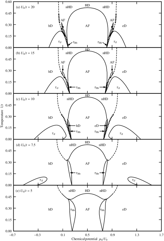
Figure 1: $d=3$ Hubbard model phase diagrams in temperature versus chemical potential. The hole-rich disordered (hD), near-half-filled disordered (nHD), half-filled disordered (HD), electron-rich disordered (eD), antiferromagnetic (AF), $\tau_{\text{Hb}}$, and $\tau_{\text{tJ}}$ phases are seen. The full curves are second-order phase boundaries, while the dotted curves are first-order boundaries. The dashed curves are not phase transitions, but disorder lines between the near-half-filled disordered and the hole-rich or electron-rich disordered phases. The progression (a) $U_{0}/t=20$ through (e) $U_{0}/t=5$ shows the changing phase diagram topology from strong to intermediate coupling. The $\tau_{\text{tJ}}$ phase, which is prominent at strong coupling, disappears entirely for $U_{0}/t\lesssim 6$, and the $\tau_{\text{Hb}}$ phase is prominent for intermediate couplings.

Figure 2: $d=3$ Hubbard model phase diagrams in temperature versus electron density. The full curves are second-order phase boundaries. The coexistence boundaries of first-order transitions are drawn with dotted curves, with the unmarked areas inside corresponding to coexistence regions of the two phases at either side. The dashed curves are not phase transitions, but disorder lines between the near-half-filled disordered and the hole-rich or electron-rich disordered phases. Noteworthy is the narrowness of the first-order transitions, with jumps in the electron density of the order of a few percent (i.e., the width of the coexistence region). The antiferromagnetic phase is unstable to about 8-15% hole (or electron) doping away from half-filling. In the intermediate $U_{0}/t$ regime, the $\tau_{{}_{\text{Hb}}}$ phase appears for about 10-18% hole (or electron) doping. At larger $U_{0}/t$, the $\tau_{{}_{\text{tJ}}}$ phase dominates, and exists between 30-35% hole (or electron) doping.

Figure 3: The data points are the calculated antiferromagnetic transition temperatures at half-filling. The linear relation that is expected for strong coupling at low temperatures (Sec.V) is obtained.

Figure 4: Comparison of the antiferromagnetic transition temperatures at half-filling for the $d=3$ Hubbard model calculated from various approaches: the renormalization-group method of the present paper (solid line); QMC Scalettar (diamonds); QMC HirschQMC (triangles); DMFT Jarrell (squares); RPA weak-coupling expansion DareAlbinet (dot-dashed line); and two approximations for the strong-coupling behavior—the high-temperature expansion of the Heisenberg model, $1/t=3.83t/U_{0}$ HirschQMC (dotted line) and Weiss mean-field theory, $1/t=6t/U_{0}$ (dashed line).

For $d=3$ and a range of couplings $U_{0}/t=5$ to $20$, Figs. 1 show Hubbard phase diagrams in terms of temperature ($1/t$) versus chemical potential ($\mu_{0}/U_{0}$). The corresponding phase diagrams in temperature ($1/t$) versus electron density $\langle n_{i}\rangle$ are in Fig. 2. The values of the interaction constants for each observed phase sink are listed in Table V. The expectation values for each phase sink, also listed in Table V, allow us to identify the phases as follows:

Hole-rich disordered (hD) phase: The electron density $\langle n_{i}\rangle$ is zero at the sink and, concomitantly, the electron densities $\langle n_{i}\rangle$ calculated inside this phase are low.

Near-half-filled disordered (nHD) phase: The basin of attraction of nHD occurs at $\mu_{0}/U_{0}\neq 1/2$. The electron density $\langle n_{i}\rangle$ is 1 at the sink and, concomitantly, the electron densities $\langle n_{i}\rangle$ calculated inside this phase are closer to half-filling. Half-filled disordered (HD) phase: The sink is for the disordered phase at perfect half-filling, $\mu_{0}/U_{0}=1/2$ and $\langle n_{i}\rangle=1$.

Electron-rich disordered (eD) phase: The electron density $\langle n_{i}\rangle$ is 2 at the sink and, concomitantly, the electron densities $\langle n_{i}\rangle$ calculated inside this phase are high.

Antiferromagnetic (AF) phase: The electron density $\langle n_{i}\rangle$ is 1 at the sink and, concomitantly, the electron densities $\langle n_{i}\rangle$ calculated inside this phase are closer to half-filling. The expectation value for the nearest-neighbor spin-spin correlation is $\langle\vec{S_{i}}\cdot\vec{S_{j}}\rangle=\frac{1}{4}$ at the sink. Note that the latter two spins are, on the original cubic lattice, distant spins on the same sublattice; from this, antiferromagnetism, $\langle\vec{S_{i}}\cdot\vec{S_{j}}\rangle<0$ when the spins are on different sublattices of the original cubic lattice, is calculationally obtained throughout this phase. Since there is no explicit antiferromagnetic coupling in the initial Hubbard Hamiltonian, the antiferromagnetic phase is completely a quantum mechanical effect resulting from the kinetic energy term. In fact, at half-filling, second-order perturbation theory in $t$, valid for small $t/U_{0}$, must yield an effective antiferromagnetic coupling proportional to $t^{2}/U_{0}$. Thus, for small $t/U_{0}$, $t^{2}/U_{0}$ should equal the same constant at all antiferromagnetic phase transitions at half-filling (Recall that all of our coupling constants are dimensionless, incorporating the inverse temperature factor $1/kT$). Equivalently, $t/U_{0}$ should be linear in $1/t$ at all antiferromagnetic phase transitions at half-filling, for small $t/U_{0}$ and therefore for small $1/t$ (low temperature):

$$1/t\>\sim\>t/U_{0}\>.$$ (16)

This is indeed rendered by our calculation, as seen in Fig. 3. For higher values of $1/t$, Eq.(16) is not applicable, since second-order perturbation theory does not hold, and indeed our calculated curve in Fig. 3 deviates from linearity. On the other hand, the approximation in our recursion relation is even more justified, since the commutation relations that are ignored involve terms of order $t^{2}$.

The antiferromagnetic transition temperature as a function of coupling $U_{0}/t$ is also shown in Fig. 4, together with calculated values from other approximation schemes for the $d=3$ Hubbard model. We see that our results for intermediate coupling are comparable to those of quantum Monte Carlo studies Scalettar ; HirschQMC . As expected, our transition temperature vanishes in the limit $U_{0}/t\to 0$, since there are no phase transitions for the non-interacting system. Thus, our approximation behaves correctly both at strong coupling (previous paragraph) and at weak coupling.

$\mathbf{\tau}_{\text{Hb}}$ and $\mathbf{\tau}_{\text{tJ}}$ phases: For large values of $U_{0}/t$, the novel phase found in the $tJ$ model FalicovBerker (which we call $\mathbf{\tau}_{\text{tJ}}$) also occurs in the Hubbard model. In addition, we find a closely related phase ($\mathbf{\tau}_{\text{Hb}}$), unique to the Hubbard model, at smaller $U_{0}/t$. The two phases are characterized by very similar properties: the hopping strengths $t_{0}$, $t_{2}$, and $t_{x}$ renormalize to $\pm\infty$, and the phase sinks have a non-zero vacancy hopping expectation value

$$\left\langle\sum_{\sigma}h_{i-\sigma}h_{j-\sigma}(c^{\dagger}_{i\sigma}c_{j\sigma}+c^{\dagger}_{j\sigma}c_{i\sigma})\right\rangle=\begin{cases}-2/3&\text{($\mathbf{\tau}_{\text{tJ}}$)}\\ 0.663972&\text{($\mathbf{\tau}_{\text{Hb}}$)}\end{cases}\>,$$ (17)

for $\mu_{0}/U_{0}<1/2$, and a non-zero pair hopping expectation value

$$\left\langle\sum_{\sigma}n_{i-\sigma}n_{j-\sigma}(c^{\dagger}_{i\sigma}c_{j\sigma}+c^{\dagger}_{j\sigma}c_{i\sigma})\right\rangle=\begin{cases}2/3&\text{($\mathbf{\tau}_{\text{tJ}}$)}\\ -0.663972&\text{($\mathbf{\tau}_{\text{Hb}}$)}\end{cases}\>,$$ (18)

for $\mu_{0}/U_{0}>1/2$. In both cases, as expected for the occurrence of hopping, the electron densities at the sinks have values different from 0 (empty), 1 (half filled), or 2 (doubly occupied): $\langle n_{i}\rangle=2/3$, $4/3$ and $\langle n_{i}n_{j}\rangle=1/3$, $5/3$ for the $\mathbf{\tau}_{\text{tJ}}$ phase, and $\langle n_{i}\rangle=0.668014$, $1.331986$ and $\langle n_{i}n_{j}\rangle=0.336028$, $1.663972$ for the $\mathbf{\tau}_{\text{Hb}}$ phase. (At the sinks of non-$\tau$ phases, the electron density is, on the other hand, 0, 1, or 2.) There are also small spin correlations in the phase sink limits, $\langle\vec{S}_{i}\cdot\vec{S}_{j}\rangle=-1/4$ for $\mathbf{\tau}_{\text{tJ}}$, and $\langle\vec{S}_{i}\cdot\vec{S}_{j}\rangle=0.0840069$ for $\mathbf{\tau}_{\text{Hb}}$, which yield, throughout these phases, small antiferromagnetic correlations in the original system.

The boundaries in Fig. 1 are controlled by fourteen unstable fixed points, given in Table VI. For smaller values of $U_{0}/t$, the topology of the phase diagram is that of Fig. 1(e), where the AF/HD, AF/nHD, AF/$\tau_{\text{Hb}}$, and hD/$\tau_{\text{Hb}}$ boundaries are respectively controlled by the second-order fixed points C${}_{1}^{\ast}$, C${}_{2}^{\ast}$, C${}_{3}^{\ast}$, and C${}_{4}^{\ast}$. The latter three boundaries intersect at the multicritical point B₂, controlled by the fixed point B${}_{2}^{\ast}$. A segment of the hD/nHD boundary just above this intersection is second-order, controlled by the fixed point C${}_{5}^{\ast}$, ending at the multicritical point B₁, controlled by the fixed point B${}_{1}^{\ast}$. The high-temperature section of the hD/nHD boundary is a disorder line, controlled by the null fixed point N*, i.e., there is no phase transition above B₁.

Phase sink	Interaction constants										Additional properties
	$t_{0}$	$t_{1}$	$t_{2}$	$t_{x}$	$U$	$\mu$	$J$	$V_{2}$	$V_{3}$	$V_{4}$
hole-rich	0	0	0	0	$\infty$	$-\infty$	0	0	0	0
disordered hD						$\mu/U=\text{const.}$
near-half-filled	$2\ln 3$	0	$-2\ln 3$	$\infty$	$\infty$	$\infty$	0	$-\infty$	$\infty$	-$\infty$	$U-2\mu-2V_{2}-V_{3}=0$
disordered nHD				$\approx 0.24U$		$\approx 0.62U$		$\approx-0.47U$	$\approx 0.69U$	$\approx-1.38U$	$2V_{3}+V_{4}=0$
half-filled	0	0	0	0	$\infty$	$\infty$	0	0	0	0	$U-2\mu=0$
disordered HD						$=\frac{1}{2}U$
electron-rich	0	0	0	0	$\infty$	$\infty$	0	0	0	0
disordered eD						$\mu/U=\text{const.}$
antiferro-	$-\infty$	0	$\infty$	$\infty$	$\infty$	$\infty$	$\infty$	$-\infty$	$\infty$	$-\infty$	$U-2\mu-2V_{2}-V_{3}\to 0$
magnetic AF	$\approx-0.29U$		$\approx 0.29U$	$\approx 0.14U$		$\approx 0.57U$	$\approx 0.29U$	$\approx-0.071U$	$V_{3}/U\to 0$	$V_{4}/U\to 0$	$2V_{3}+V_{4}\to 0$
$(\mu_{0}/U_{0}\neq 1/2)$											$t_{2}-t_{0}\to 0$
antiferro-	0	0	0	0	$\infty$	$\infty$	$\infty$	$-\infty$	$\infty$	$-\infty$	${U-2\mu-2V_{2}-V_{3}=0}$
magnetic AF						$\approx\frac{1}{2}U$	$J/U\to 0$	$\approx-\frac{1}{4}J$	$\approx\frac{1}{2}J$	$\approx-J$	$2V_{3}+V_{4}=0$
$(\mu_{0}/U_{0}=1/2)$											$t_{2}-t_{0}=0$
$\tau_{{}_{\text{Hb}}}$	$-\infty$	0	$\infty$	$-\infty$	$\infty$	$\infty$	$\infty$	$-\infty$	$-\infty$	$\infty$	$t_{0}+\mu+\frac{1}{4}J+V_{2}$
$(\mu_{0}/U_{0}<1/2)$	$\approx-\frac{1}{4}U$		$\approx\frac{1}{2}U$	$\approx-\frac{1}{2}U$		$\approx\frac{1}{4}U$	$\approx\frac{1}{2}U$	$\approx-\frac{1}{8}U$	$V_{3}/U\to 0$	$V_{4}/U\to 0$	$\qquad\approx-4.35$
$\tau_{{}_{\text{Hb}}}$	$-\infty$	0	$\infty$	$-\infty$	$\infty$	$\infty$	$\infty$	$-\infty$	$\infty$	$\infty$	$-t_{2}+U-\mu+\frac{1}{4}J$
$(\mu_{0}/U_{0}>1/2)$	$\approx-\frac{1}{2}U$		$\approx\frac{1}{4}U$	$\approx-\frac{1}{2}U$		$\approx U$	$\approx\frac{1}{2}U$	$\approx-\frac{1}{8}U$	$V_{3}/U\to 0$	$V_{4}/U\to 0$	$-V_{2}-V_{3}\approx-4.35$
$\tau_{{}_{\text{tJ}}}$	$\infty$	0	$-\infty$	$\infty$	$\infty$	$-\infty$	$-\infty$	$-\infty$	$-\infty$	$-\infty$
$(\mu_{0}/U_{0}<1/2)$	$\approx 0.13U$		$\approx-1.46U$	$\approx 0.52U$		$\approx-0.022U$	$\approx-0.87U$	$\approx-0.50U$	$\approx-1.13U$	$\approx-0.21U$
$\tau_{{}_{\text{tJ}}}$	$\infty$	0	$-\infty$	$\infty$	$\infty$	$\infty$	$-\infty$	$-\infty$	$\infty$	$-\infty$
$(\mu_{0}/U_{0}>1/2)$	$\approx 0.42U$		$\approx-0.038U$	$\approx 0.15U$		$\approx 1.62U$	$\approx-0.25U$	$\approx-0.86U$	$\approx 0.39U$	$\approx-0.060U$
Phase sink	Expectation values
	$\langle T_{0}\rangle$	$\langle T_{1}\rangle$	$\langle T_{2}\rangle$	$\langle T_{x}\rangle$	$\langle n_{i\uparrow}n_{i\downarrow}\rangle$	$\langle n_{i}\rangle$	$\langle\vec{S}_{i}\cdot\vec{S}_{j}\rangle$	$\langle n_{i}n_{j}\rangle$	$\langle n_{i\uparrow}n_{i\downarrow}n_{j}\rangle$	$\langle n_{i\uparrow}n_{i\downarrow}n_{j\uparrow}n_{j\downarrow}\rangle$
hD	0	0	0	0	0	0	0	0	0	0
nHD	0	0	0	0	0	1	0	1	0	0
HD	0	0	0	0	0	1	0	1	0	0
eD	0	0	0	0	1	2	0	4	2	1
AF	0	0	0	0	0	1	$\frac{1}{4}$	1	0	0
$\tau_{{}_{\text{Hb}}}$	$\left\{\begin{array}[]{ll}\parbox{14.45377pt}{\centering$0.663$\\ $\;\;\;972$\@add@centering}\\ 0\\ \end{array}\right.$	0	$\left\{\begin{array}[]{ll}0\\ \parbox{14.45377pt}{\centering$-0.66$\\ $\;\;3972$\@add@centering}\\ \end{array}\right.$	0	$\left\{\begin{array}[]{ll}0\\ \parbox{14.45377pt}{\centering$0.331$\\ $\;\;\;986$\@add@centering}\\ \end{array}\right.$	$\left\{\begin{array}[]{ll}\parbox{14.45377pt}{\centering$0.668$\\ $\;\;\;014$\@add@centering}\\[5.0pt] \parbox{14.45377pt}{\centering$1.331$\\ $\;\;\;986$\@add@centering}\\ \end{array}\right.$	$0.0840$ $\;\;\;069$	$\left\{\begin{array}[]{ll}\parbox{14.45377pt}{\centering$0.336$\\ $\;\;\;028$\@add@centering}\\[5.0pt] \parbox{14.45377pt}{\centering$1.663$\\ $\;\;\;972$\@add@centering}\\ \end{array}\right.$	$\left\{\begin{array}[]{ll}0\\ \parbox{14.45377pt}{\centering$0.331$\\ $\;\;\;986$\@add@centering}\\ \end{array}\right.$	0
$\tau_{{}_{\text{tJ}}}$	$\left\{\begin{array}[]{ll}-\frac{2}{3}\\ 0\\ \end{array}\right.$	0	$\left\{\begin{array}[]{ll}0\\ \frac{2}{3}\\ \end{array}\right.$	0	$\left\{\begin{array}[]{ll}0\\ \frac{1}{3}\\ \end{array}\right.$	$\left\{\begin{array}[]{ll}\frac{2}{3}\\ \frac{4}{3}\\ \end{array}\right.$	$-\frac{1}{4}$	$\left\{\begin{array}[]{ll}\frac{1}{3}\\ \frac{5}{3}\\ \end{array}\right.$	$\left\{\begin{array}[]{ll}0\\ \frac{1}{3}\\ \end{array}\right.$	0

Table V: Interaction constants and expectation values at the phase sink fixed points. For $\tau_{{}_{\text{Hb}}}$ and $\tau_{{}_{\text{tJ}}}$, the values for $\mu_{0}/U_{0}{<\atop>}\frac{1}{2}$ are given. The hopping expectation values $\langle T_{\alpha}\rangle$ are: $\langle T_{0}\rangle=\sum_{\sigma}\langle h_{i-\sigma}h_{j-\sigma}(c^{\dagger}_{i\sigma}c_{j\sigma}+c^{\dagger}_{j\sigma}c_{i\sigma})\rangle$, $\langle T_{1}\rangle=\sum_{\sigma}\langle(n_{i\,-\sigma}h_{j\,-\sigma}+h_{i\,-\sigma}n_{j\,-\sigma})(c^{\dagger}_{i\sigma}c_{j\sigma}+c^{\dagger}_{j\sigma}c_{i\sigma})\rangle$, $\langle T_{2}\rangle=\sum_{\sigma}\langle n_{i\,-\sigma}n_{j\,-\sigma}(c^{\dagger}_{i\sigma}c_{j\sigma}+c^{\dagger}_{j\sigma}c_{i\sigma})\rangle$, $\langle T_{x}\rangle=\langle c^{\dagger}_{i\uparrow}c_{j\uparrow}c^{\dagger}_{i\downarrow}c_{j\downarrow}+c^{\dagger}_{j\uparrow}c_{i\uparrow}c^{\dagger}_{j\downarrow}c_{i\downarrow}\rangle$.

Basin

Type

Interaction constants

Additional properties

Relevant eigenvalue exponents (y)

$t_{0}$

$t_{1}$

$t_{2}$

$t_{x}$

$U$

$\mu$

$J$

$V_{2}$

$V_{3}$

$V_{4}$

$F_{1}^{\ast}$

portion of

1st

$2\ln 3$

0

$-2\ln 3$

$\infty$

$\infty$

$-\infty$

0

$\infty$

$-\infty$

$-\infty$

$2\mu+V_{2}\approx-0.396$

3

hD/nHD

order

$U-2\mu-2V_{2}-V_{3}\to 0$

boundary

$F_{2}^{\ast}$

AF/hD

1st

$-\infty$

0

$\infty$

$\infty$

$\infty$

$-\infty$

$\infty$

$\infty$

$-\infty$

$\infty$

$U-2\mu-2V_{2}-V_{3}\to 0$

3

boundary

order

$8\mu+J+4V_{2}\approx-0.658$

$C_{1}^{\ast}$

AF/HD

2nd

0

0

0

0

$\infty$

$\infty$

1.376

$-0.0650$

$0.130$

$-0.260$

$U-2\mu-2V_{2}-V_{3}=0$

0.715

boundary

order

$\approx\frac{1}{2}U$

$2V_{3}+V_{4}=0$

$C_{2}^{\ast}$

AF/nHD

2nd

$-0.554$

0

0.554

$\infty$

$\infty$

$\infty$

1.376

$-\infty$

$\infty$

$-\infty$

$U-2\mu-2V_{2}-V_{3}\to 0$

0.715

boundary

order

$2V_{3}+V_{4}\to 0$

$C_{3}^{\ast}$

AF/$\tau_{{}_{\text{Hb}}}$

2nd

$-\infty$

0

$\infty$

$-\infty$

$\infty$

$\infty$

$\infty$

$-\infty$

$\infty$

$-\infty$

$t_{0}+\mu+\frac{1}{4}J+V_{2}\approx-0.739$

1.68

boundary

order

$C_{4}^{\ast}$

hD/$\tau_{{}_{\text{Hb}}}$

2nd

$-\infty$

0

$\infty$

$-\infty$

$\infty$

$-\infty$

$\infty$

$\infty$

$-\infty$

$\infty$

$t_{0}+\mu+\frac{1}{4}J+V_{2}\approx-5.178$

1.42

boundary

order

$8\mu+J+4V_{2}\approx 6.617$

$C_{5}^{\ast}$

portion of

2nd

$-1.610$

0

$-2\ln 3$

$-1.594$

$\infty$

0.523

0

0.0108

$-0.569$

$-\infty$

1.56

hD/nHD

order

$\approx-3U$

boundary

$C_{6}^{\ast}$

hD/$\tau_{{}_{\text{tJ}}}$

2nd

$2.959$

0

$-29.585$

$9.629$

$\infty$

$1.016$

$-13.692$

$-8.332$

$-18.259$

$-\infty$

1.01

boundary

order

$N^{\ast}$

portion of

null

0

0

$-2\ln 3$

0

$\infty$

0

0

0

$4\ln\frac{\sqrt{3}}{2}$

$-\infty$

2

hD/nHD

$\approx-3U$

boundary

$L^{\ast}$

$F_{1}^{\ast}$, $F_{2}^{\ast}$, $C_{2}^{\ast}$

critical

$-0.554$

0

0.554

$\infty$

$\infty$

$-\infty$

1.376

$\infty$

$-\infty$

$-\infty$

$U-2\mu-2V_{2}-V_{3}\to 0$

3

basins meet

endpoint

$8\mu+J+4V_{2}\approx-0.798$

0.715155

$B_{1}^{\ast}$

$C_{5}^{\ast}$, $N^{\ast}$

multi-

$-1.236$

0

$-2\ln 3$

$-1.005$

$\infty$

0.221

0

0.127

$-0.652$

$-\infty$

1.73

basins meet

critical

$\approx-3U$

0.22

$B_{2}^{\ast}$

$C_{2}^{\ast}$, $C_{3}^{\ast}$, $C_{4}^{\ast}$,

multi-

$-2.156$

0

$-1.555$

$-2.708$

$\infty$

$1.559$

$0.321$

$-0.762$

$0.201$

$-\infty$

1.15

$C_{5}^{\ast}$ basins meet

critical

$\approx-3U$

0.27

$B_{3}^{\ast}$

$F_{1}^{\ast}$, $N^{\ast}$

multi-

0

0

$-2\ln 3$

0

$\infty$

$-0.681$

0

$1.089$

$-0.438$

$-\infty$

$3U+V_{4}\approx 3.044$

2.56

basins meet

critical

$\approx-3U$

0.96

$B_{4}^{\ast}$

$F_{2}^{\ast}$, $C_{3}^{\ast}$, $C_{4}^{\ast}$

multi-

$-\infty$

0

$\infty$

$-\infty$

$\infty$

$-\infty$

$\infty$

$\infty$

$-\infty$

$-\infty$

$t_{0}+\mu+\frac{1}{4}J+V_{2}\to 0$

2.68

basins meet

critical

$8\mu+J+4V_{2}\to 0$

1.90

Table VI: Unstable fixed points. The fixed points of the $\mu_{0}/U_{0}\leq 1/2$ half space are given here.

As $U_{0}/t$ is increased, the phase diagram topology becomes more complex. For $U_{0}/t\gtrsim 6$, the $\tau_{\text{tJ}}$ phase appears, its boundary with hD controlled by the second-order fixed point C${}_{6}^{\ast}$. Portions of the lower-temperature boundary between the hD and nHD phases become first-order (fixed point F${}_{1}^{\ast}$), and islands of AF appear above the $\tau_{\text{tJ}}$ phase; their boundaries with hD are also first-order (fixed point F${}_{2}^{\ast}$). The intersections of these first-order boundaries with other phase boundaries are controlled by the additional multicritical points $B_{3}^{\ast}$ and $B_{4}^{\ast}$, and by the critical endpoint $L^{\ast}$ BerkerWortis .

As the coupling $U_{0}/t$ varies, a most interesting aspect of the changing phase diagram topology is the relative sizes of the $\tau_{\text{hB}}$ and $\tau_{\text{tJ}}$ phases. The $\tau_{\text{hB}}$ phase is largest at intermediate values of $U_{0}/t$, and gradually decreases in size as we move into the strong-coupling regime, breaking up into narrow slivers until at large values of $U_{0}/t$ only tiny remnants of it are left in the phase diagram. The $\tau_{\text{tJ}}$ phase appears at intermediate values of $U_{0}/t$, grows in size as $U_{0}/t$ is increased, and occupies a prominent place in the diagram next to the AF phase in the strong-coupling regime. As discussed in Section VII, this is precisely what we expect, since the Hubbard phase diagram should approximately reproduce the $tJ$ model results FalicovBerker in the large $U_{0}/t$ limit.

Phase diagrams in terms of temperature versus electron density $\langle n_{i}\rangle$ are shown in Fig. 2. It is seen that the antiferromagnetic phase is unstable to at most 15% hole (or electron) doping at low temperatures. The $\tau_{{}_{\text{Hb}}}$ and $\tau_{{}_{\text{tJ}}}$ phases exist at different doping values, with $\tau_{{}_{\text{Hb}}}$ appearing for approximately 10-18% doping, directly adjacent to the AF phase, and $\tau_{{}_{\text{tJ}}}$ in the 30-35% doping range. The narrowness of the first-order transitions, with jumps in the electron density of the order of a few percent, is noteworthy.

VI Specific Heat Results

From the calculated expectation values of the operators occurring in the Hamiltonian [Eq.(2)], we have obtained the dimensionless internal energy per bond $\langle\beta H(i,j)\rangle$. Recall that dimensionless coupling constants are exhibited in the Hubbard Hamiltonian of Eq.(2), e.g.,

$$t=\frac{\tilde{t}}{k_{B}T}\,,$$ (19)

where $\tilde{t}$ is a constant that does not depend on temperature. The specific heat is calculated with

$$C=\frac{\partial\langle H(i,j)\rangle}{\partial T}=k_{B}\left\{\frac{\partial}{\partial t^{-1}}\langle c^{\dagger}_{i\sigma}c_{j\sigma}+c^{\dagger}_{j\sigma}c_{i\sigma}\rangle\right.\\ +\left.\frac{U}{t}\frac{\partial}{\partial t^{-1}}\langle n_{i\uparrow}n_{i\downarrow}+n_{j\uparrow}n_{j\downarrow}\rangle\right\}.$$ (20)

The partial derivatives are taken at fixed $U_{0}/t$ and at fixed density $\langle n_{i}\rangle$.

In Fig. 5 we plot $\gamma=C/T$ for $U_{0}/t=15$ at several different electron densities. (The corresponding phase diagram is shown in Fig. 2(b)). At half-filling, $\langle n_{i}\rangle=1.00$, we observe a broad peak near the HD/AF transition temperature, which we can attribute to the onset of spin order. As we dope the system with holes, this peak gets sharper, becoming most pronounced near $\langle n_{i}\rangle=0.68$, directly above the transition temperature between the hD and $\tau_{{}_{\text{tJ}}}$ phases. In fact, the $C/T$ curve shows a multipeak structure near the transition, a general characteristic of the phase diagram region just above the $\tau_{{}_{\text{tJ}}}$ phase. At electron density $\langle n_{i}\rangle=0.60$, no longer in the $\tau_{{}_{\text{tJ}}}$ range, the peak decreases in size and broadens out again.

The distinct nature of the $\tau_{{}_{\text{tJ}}}$ and $\tau_{{}_{\text{Hb}}}$ phases becomes clear when we look at the low temperature specific heat. In Fig. 6 we plot the coefficient $\gamma=C/T$ as a function of electron density for $U_{0}/t=15$ and at low temperature $1/t=0.085$. In the limit as $T\to 0$, $\gamma$ is a measure of the linear contribution to the specific heat due to quasiparticle excitations. Near half-filling, $\gamma$ is close to zero, increases to a small level with sufficient hole doping, falls to near zero again in the $\tau_{{}_{\text{Hb}}}$ phase, and dramatically increases only after the system makes a narrow first-order transition to the hole-rich disordered phase. The steady rise of $\gamma$ in the hD phase with further hole doping is consistent with a Fermi liquid interpretation of this phase. The increase in $\gamma$ is interrupted by the $\tau_{{}_{\text{tJ}}}$ interval, where the curve makes a sharp oscillation, but continues in the hD region on the other side.

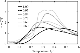
Figure 5: The specific heat coefficient $\gamma=C/T$ as a function of temperature for $U_{0}/t=15$, at several different electron densities $\langle n_{i}\rangle$ indicated in the legend. For this temperature range the densities $\langle n_{i}\rangle=1.00$ and $0.93$ lie inside the antiferromagnetic (AF) phase, $0.84$ inside the $\tau_{{}_{\text{Hb}}}$ phase, $0.73$ and $0.60$ inside the hole-rich disordered (hD) phase, and $0.68$ inside the $\tau_{{}_{\text{tJ}}}$ phase. Here and in the following figures, $\gamma$ is shown in units of $k_{B}^{2}/\tilde{t}$, where $\tilde{t}$ is the temperature-independent constant in Eq. (19).

Figure 6: The specific heat coefficient $\gamma=C/T$ for $U_{0}/t=15$ at the low temperature of $1/t=0.085$, as a function of electron density $\langle n_{i}\rangle$. The corresponding phases are indicated near the top of the figure, with second-order phase boundaries marked by thin vertical lines. The interval between the vertical dashed lines corresponds to the first-order phase transition.

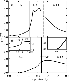
Figure 7: The specific heat coefficient $\gamma=C/T$ as a function of temperature for two different electron densities and values of $U_{0}/t$: (a) $\langle n_{i}\rangle=0.68$, $U_{0}/t=20$; (b) $\langle n_{i}\rangle=0.875$, $U_{0}/t=7.5$. Phases are indicated near the top of the figures, with second-order phase boundaries marked by thin vertical lines. The interval between the vertical dashed lines corresponds to a first-order phase transition. In diagram (b) the top left inset shows a close-up of the cusp in $\gamma$ at the AF/$\tau_{{}_{\text{Hb}}}$ transition temperature. The data points in the top right inset are calculated $\gamma$ values for temperatures $1/t<0.2$, fitted to a BCS-like exponential curve of the form $C/k_{B}T=\frac{A}{T^{5/2}}\exp\left(-\frac{\Delta}{T}\right)$, with best-fit parameters $A=1.02\pm 0.06$ and $\Delta=1.01\pm 0.01$, where $t^{-1}$ is used as the temperature variable.

We see that the $\tau_{{}_{\text{tJ}}}$ phase has non-zero $\gamma$ at low temperatures, while the $\tau_{{}_{\text{Hb}}}$ phase does not. In Figs. 7(a) and (b) we contrast the two $\tau$ phases directly, comparing representative $C/T$ curves for $\tau_{{}_{\text{tJ}}}$ and $\tau_{{}_{\text{Hb}}}$ transitions. We observe that in the $\tau_{{}_{\text{Hb}}}$ phase the low-temperature specific heat exhibits an exponential form characteristic of a gap in the quasiparticle spectrum. Specific heat data points for temperatures $1/t<0.2$, shown in the top right inset of Fig. 7(b), were found to fit a theoretical curve of the same form as in the $T\to 0$ limit of a weakly-coupled, BCS-type superconductor,

$$\frac{C}{k_{B}}=\frac{A}{T^{3/2}}\exp\left(-\frac{\Delta}{T}\right)\,,$$ (21)

with a best-fit coefficient $A=1.02\pm 0.06$ and a zero-temperature gap $\Delta=1.01\pm 0.01$, where $t^{-1}$ is used as the temperature variable. In contrast, the $\tau_{{}_{\text{tJ}}}$ phase clearly has a gapless spectrum, as we see in the $C/T$ curve of Fig. 7(a). As mentioned earlier, we also clearly see multiple peaks in the specific heat just above the hD/$\tau_{{}_{\text{tJ}}}$ transition temperature.

The $\tau_{{}_{\text{tJ}}}$ and $\tau_{{}_{\text{Hb}}}$ phases have similar properties at the phase sink, most notably a non-zero hopping amplitude, and thus are both good candidates for superconductivity. Since the two phases are dominant in different $U_{0}/t$ regimes, their contrasting specific heat characteristics can potentially be understood as the difference between strongly-coupled and weakly-coupled superconducting phases. For the strongly-coupled, BEC-like case, pairing occurs above $T_{c}$, and these tightly bound bosonic pairs condense at the transition temperature. The double-peak structure in the specific heat above the $\tau_{{}_{\text{tJ}}}$ phase is a possible indicator of such pair formation. Additionally, we expect that a BEC-like superconducting transition in three dimensions should have a specific heat critical exponent $\alpha=-1$ Junod . Analysis of the $C_{6}^{\ast}$ fixed point, governing the hD/$\tau_{{}_{\text{tJ}}}$ boundary, yields the result $\alpha=-0.97$. The presence of low-lying excitations in a Bose gas is also consistent with the fact that we do not see a gap in the low-temperature specific heat of the $\tau_{{}_{\text{tJ}}}$ phase.

Turning now to the $\tau_{{}_{\text{Hb}}}$ phase, we already noted that its specific heat can be closely fitted at low temperatures to a BCS-like exponential curve, which is exactly what we would expect for a weakly-coupled superconducting phase. Analysis of the $C_{3}^{\ast}$ fixed point, controlling the AF/$\tau_{{}_{\text{Hb}}}$ boundary, yields a specific heat coefficient $\alpha=-0.27$. This translates into a finite cusp at the transition temperature, as shown in the top left inset of Fig. 7(b). For weak and intermediate couplings the superconducting transition is expected to belong to the universality class of the $d=3$ $XY$ model, with $\alpha=-0.013$ Lipa (examples of transitions in this class include the superfluid transition of ⁴He, the superconducting transition in certain high-$T_{c}$ materials like Y-123, and also in conventional superconductors, though for the latter the critical region is too narrow to be observed experimentally) Junod . Our calculated $\alpha$ is closer to the $d=3$ $XY$ than to the BEC value, supporting the weak-coupling interpretation of the $\tau_{{}_{\text{Hb}}}$ phase.

VII The $tJ$ Limit of the Hubbard Model

Figure 8: $d=3$ Hubbard model phase diagram for large Coulomb repulsion $U_{0}/t=50$ in temperature versus (a) chemical potential, (b) electron density $\langle n_{i}\rangle$. The full curves are second-order phase boundaries, while the dotted curves indicate first-order boundaries. The dashed lines are not phase transitions, but disorder lines between the near-half-filled disordered and hole-rich disordered phases.

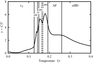
Figure 9: The specific heat coefficient $\gamma=C/T$ as a function of temperature for $U_{0}/t=50$ and $\langle n_{i}\rangle=0.67$. Phases are indicated near the top of the figure, with second-order phase boundaries marked by thin vertical lines. The dashed lines are not phase transitions, but disorder lines between the near-half-filled disordered and hole-rich disordered phases.

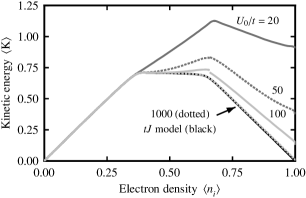
Figure 10: The kinetic energy per bond $\langle K\rangle=-\sum_{\sigma}\langle c_{i\sigma}^{\dagger}c_{j\sigma}+c_{j\sigma}^{\dagger}c_{i\sigma}\rangle$ as a function of electron density $\langle n_{i}\rangle$ at temperature $1/t=0.2$ for Coulomb repulsions $U_{0}/t=20$, 50, 100, and 1000 (indicated by numbers next to each curve). The solid curve at the bottom is the result calculated using the $tJ$ model renormalization-group equations FalicovBerker ; FalicovBerkerT at the same temperature, with the corresponding $J/t=0.004$.

In the strong-coupling limit $U_{0}\gg t$, second-order perturbation theory in $t/U_{0}$ applied to the Hubbard model leads to the following Hamiltonian (known as the $tJ$ model) Anderson ; BZA ; FalicovBerker ; FalicovBerkerT ; Chao ; Hirsch2 ; LMFalicov ; RabeBhatt ; Bares ,

$$H_{\text{$tJ$}}=-t\sum_{\langle ij\rangle,\sigma}P\left(c_{i\sigma}^{\dagger}c_{j\sigma}+c_{j\sigma}^{\dagger}c_{i\sigma}\right)P\\ +J\sum_{\langle ij\rangle}(\vec{S}_{i}\cdot\vec{S}_{j}-\frac{1}{4}n_{i}n_{j})\,,$$ (22)

where $J=4t^{2}/U$ and $P$ is a projection operator prohibiting double occupation of a lattice site. In addition to the terms shown above, the perturbation theory generates a three-site term of the form $\sum_{\langle ikj\rangle}c^{\dagger}_{i\sigma}(S_{k})_{\sigma\sigma^{\prime}}c_{j\sigma^{\prime}}$, but this term is usually ignored, from the assumption that it does not radically alter the physics of the $tJ$ model. (Our current results, directly from the strong-coupling limit of the actual Hubbard model, confirm this assumption.) We thus expect that our Hubbard model approach in the limit of large $U_{0}/t$ should give results qualitatively similar to those found for the $tJ$ model in earlier renormalization-group studies FalicovBerker ; FalicovBerkerT . The phases of the $tJ$ model found in these studies are identical to those of the Hubbard model, except that there is no $\tau_{{}_{\text{Hb}}}$ phase.

Fig. 8 shows the Hubbard model phase diagram in terms of temperature versus chemical potential and temperature versus electron density for $U_{0}/t=50$. At this large coupling, we do indeed observe a phase diagram very similar to that found in the earlier study of the $tJ$ model FalicovBerker ; FalicovBerkerT . In particular, the $\tau_{\text{\text{tJ}}}$ phase is surrounded by AF islands, and directly above $\tau_{\text{\text{tJ}}}$ we get a lamellar structure of alternating AF, nHD, and hD phases. The AF phase near half-filling is unstable to only about 5% hole doping. This phase diagram can be seen as an evolution from the $U_{0}/t=20$ result of Figs. 1(a) and 2(a), with the $\tau_{\text{\text{hB}}}$ entirely disappearing at $U_{0}/t=50$ except for infinitesimal slivers. The multiple peaks in the specific heat above the $\tau_{\text{\text{tJ}}}$ transition persist in the strong-coupling limit, as seen in Fig. 9, which plots the specific heat coefficient $\gamma$ for $U/t_{0}=50$ at $\langle n_{i}\rangle=0.67$. The peak structure here is more complex than in Fig. 7(a), due to the above-mentioned lamellar phases.

We can also observe the evolution from the Hubbard to the $tJ$ limits through the expectation value of the kinetic energy per bond, $\langle K\rangle=-\sum_{\sigma}\langle c_{i\sigma}^{\dagger}c_{j\sigma}+c_{j\sigma}^{\dagger}c_{i\sigma}\rangle$, which is proportional to the density of free carriers in the system. Fig. 10 shows $\langle K\rangle$ as a function of electron density for the temperature $1/t=0.2$, calculated at several different couplings $U_{0}/t$. As $U_{0}/t$ is increased, the value of $\langle K\rangle$ at half-filling is reduced, and when $U_{0}/t=1000$ we are close to the $tJ$ limit, with the kinetic energy at half-filling almost zero, indicating no available free carriers due to the prohibitively high energy of double occupation. The $U_{0}/t=1000$ curve almost exactly overlaps the result calculated from the $tJ$ model renormalization-group equations at the same temperature using the corresponding coupling $J/t=4t/U_{0}=0.004$.

Appendix A: Determination of the $\gamma_{p}$       in Terms of the Matrix Elements        of the Three-Site Hamiltonian

Eq.(8) allows us to express the matrix elements $\gamma_{p}\equiv\langle\phi_{p}|e^{-\beta^{\prime}H^{\prime}(i,k)}|\phi_{p}\rangle$ of the renormalized, exponentiated two-site Hamiltonian in terms of matrix elements of the unrenormalized, exponentiated three-site Hamiltonian, as given below. The $\gamma_{p}$, in turn, determine the renormalized interaction constants, in Eq.(10). In the equations below, $\langle\psi_{q}||\psi_{\bar{q}}\rangle$ denotes $\langle\psi_{q}|e^{-\beta H(i,j)-\beta H(j,k)}|\psi_{\bar{q}}\rangle$:

$$\gamma_{1}= \langle\psi_{1}||\psi_{1}\rangle+2\langle\psi_{2}||\psi_{2}\rangle+\langle\psi_{9}||\psi_{9}\rangle,$$

$$\gamma_{2}= \langle\psi_{3}||\psi_{3}\rangle+\frac{1}{2}\langle\psi_{8}||\psi_{8}\rangle+\frac{3}{2}\langle\psi_{15}||\psi_{15}\rangle+\langle\psi_{24}||\psi_{24}\rangle,$$

$$\gamma_{4}= \langle\psi_{6}||\psi_{6}\rangle+\frac{1}{2}\langle\psi_{11}||\psi_{11}\rangle+\frac{3}{2}\langle\psi_{20}||\psi_{20}\rangle+\langle\psi_{32}||\psi_{32}\rangle,$$

$$\gamma_{6}= \langle\psi_{10}||\psi_{10}\rangle+2\langle\psi_{26}||\psi_{26}\rangle+\langle\psi_{44}||\psi_{44}\rangle,$$

$$\gamma_{7}= \langle\psi_{13}||\psi_{13}\rangle+\langle\psi_{34}||\psi_{34}\rangle+\langle\psi_{38}||\psi_{38}\rangle+\langle\psi_{48}||\psi_{48}\rangle,$$

$$\gamma_{8}= \langle\psi_{12}||\psi_{12}\rangle+2\langle\psi_{31}||\psi_{31}\rangle+\langle\psi_{47}||\psi_{47}\rangle,$$

$$\gamma_{9}= \langle\psi_{14}||\psi_{14}\rangle+\frac{2}{3}\langle\psi_{23}||\psi_{23}\rangle+\frac{4}{3}\langle\psi_{39}||\psi_{39}\rangle+\langle\psi_{49}||\psi_{49}\rangle,$$

$$\gamma_{12}= \langle\psi_{25}||\psi_{25}\rangle+\frac{1}{2}\langle\psi_{45}||\psi_{45}\rangle+\frac{3}{2}\langle\psi_{50}||\psi_{50}\rangle+\langle\psi_{59}||\psi_{59}\rangle,$$

$$\gamma_{14}= \langle\psi_{33}||\psi_{33}\rangle+\frac{1}{2}\langle\psi_{46}||\psi_{46}\rangle+\frac{3}{2}\langle\psi_{55}||\psi_{55}\rangle+\langle\psi_{62}||\psi_{62}\rangle,$$

$$\gamma_{16}= \langle\psi_{43}||\psi_{43}\rangle+2\langle\psi_{58}||\psi_{58}\rangle+\langle\psi_{64}||\psi_{64}\rangle,$$

$$\gamma_{0}\equiv \langle\phi_{6}|e^{-\beta^{\prime}H^{\prime}(i,k)}|\phi_{8}\rangle$$

$$= \langle\psi_{10}||\psi_{12}\rangle+2\langle\psi_{26}||\psi_{31}\rangle+\langle\psi_{44}||\psi_{47}\rangle.$$

References

- (1) J. Hubbard, Proc. R. Soc. A 276, 238 (1963); 277, 237 (1964); 281, 401 (1964).
- (2) G. Migliorini and A.N. Berker, Eur. Phys. J. B 17, 3 (2000).
- (3) K.G. Wilson, Phys. Rev. B 4, 3174, 3184 (1971).
- (4) J.E. Hirsch, Phys. Rev. B 22, 5259 (1980).
- (5) B. Fourcade and G. Spronken, Phys. Rev. B 29, 5012, 5089, 5096 (1984).
- (6) C. Vanderzande and A.L. Stella, J. Phys. C 17, 2075 (1984).
- (7) C. Vanderzande, J. Phys. A 18, 889 (1985).
- (8) S.A. Cannas, F.A. Tamarit, and C. Tsallis, Solid State Commun. 78, 685 (1991).
- (9) S.A. Cannas and C. Tsallis, Z. Phys. 89, 195 (1992).
- (10) A.C. Cosentini, M. Capone, L. Guidoni, and G. Bachelet, Phys. Rev. B 58, 18235 (1998).
- (11) P.W. Anderson, Science 235, 1196 (1987).
- (12) G. Baskaran, Z. Zhou, and P.W. Anderson, Solid State Commun. 63, 973 (1987).
- (13) A. Falicov and A.N. Berker, Phys. Rev. B 51, 12458 (1995).
- (14) A. Falicov and A.N. Berker, Turk. J. Phys. 19, 127 (1995).
- (15) F.C. Chou and D.C. Johnston, Phys. Rev. B 54, 572 (1996).
- (16) J. Solyom, Adv. Phys. 28, 201 (1979).
- (17) J. Voit, Rep. Prog. Phys. 57, 977 (1994).
- (18) D. Zanchi and H.J. Schulz, Europhys. Lett. 44, 235 (1997).
- (19) D. Zanchi and H.J. Schulz, Phys. Rev. B 61, 13609 (2000).
- (20) C.J. Halboth and W. Metzner, Phys. Rev. B 61, 7364 (2000).
- (21) C.J. Halboth and W. Metzner, Phys. Rev. Lett. 85, 5162 (2000).
- (22) C. Honerkamp, M. Salmhofer, N. Furukawa, and T.M. Rice, Phys. Rev. B 63, 035109 (2001).
- (23) C. Honerkamp, M. Salmhofer, and T.M. Rice, Eur. Phys. J. B 27, 127 (2002).
- (24) A. Junod, A. Erb, and C. Renner, Physica C 317-318, 333 (1999).
- (25) M. Suzuki and H. Takano, Phys. Lett. A 69, 426 (1979).
- (26) H. Takano and M. Suzuki, J. Stat. Phys. 26, 635 (1981).
- (27) A.A. Migdal, Zh. Eksp. Teor. Fiz. 69, 1457 (1975) [Sov. Phys. JETP 42, 743 (1976)].
- (28) L.P. Kadanoff, Ann. Phys. (N.Y.) 100, 359 (1976).
- (29) G.S. Rushwood and P.J. Wood, Mol. Phys. 6, 409 (1963).
- (30) J. Oitmaa and W. Zheng, J. Phys.: Condens. Matter 16, 8653 (2004).
- (31) A.N. Berker and M. Wortis, Phys. Rev. B 14, 4946 (1976).
- (32) A.N. Berker, S. Ostlund, and F.A. Putnam, Phys. Rev. B 17, 3650 (1978).
- (33) R.T. Scalettar, D.J. Scalapino, R.L. Sugar, and D. Toussaint, Phys. Rev. B 39, 4711 (1989).
- (34) J.E. Hirsch, Phys. Rev. B 35, 1851 (1987).
- (35) M. Jarrell, Phys. Rev. Lett. 69, 168 (1992).
- (36) A-M. Daré and G. Albinet, Phys. Rev. B 61, 4567 (2000).
- (37) J.A. Lipa, D.R. Swanson, J.A. Nissen, T.C.P. Chui, and U.E. Israelsson, Phys. Rev. Lett. 76, 944 (1996).
- (38) K.A. Chao, J. Spalek, and A.M. Oles, J. Phys. C 10, L271 (1977).
- (39) J.E. Hirsch, Phys. Rev. Lett. 54, 1317 (1985).
- (40) J.K. Freericks and L.M. Falicov, Phys. Rev. B 42, 4960 (1990).
- (41) K.M. Rabe and R.N. Bhatt, J. Appl. Phys. 69, 4508, (1991).
- (42) P.M. Bares, G. Blatter, and M. Ogata, Phys. Rev. B 44, 130 (1991).